Discover how to develop a deep convolutional neural network model from scratch for the CIFAR-10 object classification dataset.
The CIFAR-10 small photo classification problem is a standard dataset used in computer vision and deep learning.
Although the dataset is effectively solved, it can be used as the basis for learning and practicing how to develop, evaluate, and use convolutional deep learning neural networks for image classification from scratch.
This includes how to develop a robust test harness for estimating the performance of the model, how to explore improvements to the model, and how to save the model and later load it to make predictions on new data.
In this tutorial, you will discover how to develop a convolutional neural network model from scratch for object photo classification.
After completing this tutorial, you will know:
How to develop a test harness to develop a robust evaluation of a model and establish a baseline of performance for a classification task.
How to explore extensions to a baseline model to improve learning and model capacity.
How to develop a finalized model, evaluate the performance of the final model, and use it to make predictions on new images.
Kick-start your project with my new book Deep Learning for Computer Vision, including step-by-step tutorials and the Python source code files for all examples.
Let’s get started.
Updated Oct/2019: Updated for Keras 2.3 and TensorFlow 2.0.
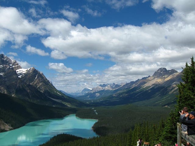
How to Develop a Convolutional Neural Network From Scratch for CIFAR-10 Photo Classification Photo by Rose Dlhopolsky, some rights reserved.
Tutorial Overview
This tutorial is divided into six parts; they are:
CIFAR-10 Photo Classification Dataset
Model Evaluation Test Harness
How to Develop a Baseline Model
How to Develop an Improved Model
How to Develop Further Improvements
How to Finalize the Model and Make Predictions
Want Results with Deep Learning for Computer Vision?
Take my free 7-day email crash course now (with sample code).
Click to sign-up and also get a free PDF Ebook version of the course.
The dataset is comprised of 60,000 32×32 pixel color photographs of objects from 10 classes, such as frogs, birds, cats, ships, etc. The class labels and their standard associated integer values are listed below.
0: airplane
1: automobile
2: bird
3: cat
4: deer
5: dog
6: frog
7: horse
8: ship
9: truck
These are very small images, much smaller than a typical photograph, and the dataset was intended for computer vision research.
CIFAR-10 is a well-understood dataset and widely used for benchmarking computer vision algorithms in the field of machine learning. The problem is “solved.” It is relatively straightforward to achieve 80% classification accuracy. Top performance on the problem is achieved by deep learning convolutional neural networks with a classification accuracy above 90% on the test dataset.
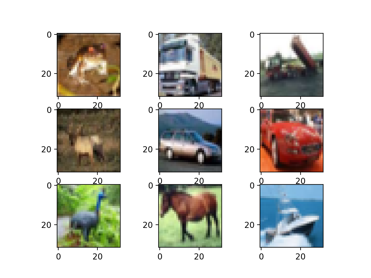
The example below loads the CIFAR-10 dataset using the Keras API and creates a plot of the first nine images in the training dataset.
Running the example loads the CIFAR-10 train and test dataset and prints their shape.
We can see that there are 50,000 examples in the training dataset and 10,000 in the test dataset and that images are indeed square with 32×32 pixels and color, with three channels.
1
2
Train: X=(50000, 32, 32, 3), y=(50000, 1)
Test: X=(10000, 32, 32, 3), y=(10000, 1)
A plot of the first nine images in the dataset is also created. It is clear that the images are indeed very small compared to modern photographs; it can be challenging to see what exactly is represented in some of the images given the extremely low resolution.
This low resolution is likely the cause of the limited performance that top-of-the-line algorithms are able to achieve on the dataset.
Plot of a Subset of Images From the CIFAR-10 Dataset
Model Evaluation Test Harness
The CIFAR-10 dataset can be a useful starting point for developing and practicing a methodology for solving image classification problems using convolutional neural networks.
Instead of reviewing the literature on well-performing models on the dataset, we can develop a new model from scratch.
The dataset already has a well-defined train and test dataset that we will use. An alternative might be to perform k-fold cross-validation with a k=5 or k=10. This is desirable if there are sufficient resources. In this case, and in the interest of ensuring the examples in this tutorial execute in a reasonable time, we will not use k-fold cross-validation.
The design of the test harness is modular, and we can develop a separate function for each piece. This allows a given aspect of the test harness to be modified or interchanged, if we desire, separately from the rest.
We can develop this test harness with five key elements. They are the loading of the dataset, the preparation of the dataset, the definition of the model, the evaluation of the model, and the presentation of results.
Load Dataset
We know some things about the dataset.
For example, we know that the images are all pre-segmented (e.g. each image contains a single object), that the images all have the same square size of 32×32 pixels, and that the images are color. Therefore, we can load the images and use them for modeling almost immediately.
1
2
# load dataset
(trainX,trainY),(testX,testY)=cifar10.load_data()
We also know that there are 10 classes and that classes are represented as unique integers.
We can, therefore, use a one hot encoding for the class element of each sample, transforming the integer into a 10 element binary vector with a 1 for the index of the class value. We can achieve this with the to_categorical() utility function.
1
2
3
# one hot encode target values
trainY=to_categorical(trainY)
testY=to_categorical(testY)
The load_dataset() function implements these behaviors and can be used to load the dataset.
1
2
3
4
5
6
7
8
# load train and test dataset
def load_dataset():
# load dataset
(trainX,trainY),(testX,testY)=cifar10.load_data()
# one hot encode target values
trainY=to_categorical(trainY)
testY=to_categorical(testY)
returntrainX,trainY,testX,testY
Prepare Pixel Data
We know that the pixel values for each image in the dataset are unsigned integers in the range between no color and full color, or 0 and 255.
We do not know the best way to scale the pixel values for modeling, but we know that some scaling will be required.
A good starting point is to normalize the pixel values, e.g. rescale them to the range [0,1]. This involves first converting the data type from unsigned integers to floats, then dividing the pixel values by the maximum value.
1
2
3
4
5
6
# convert from integers to floats
train_norm=train.astype('float32')
test_norm=test.astype('float32')
# normalize to range 0-1
train_norm=train_norm/255.0
test_norm=test_norm/255.0
The prep_pixels() function below implement these behaviors and is provided with the pixel values for both the train and test datasets that will need to be scaled.
1
2
3
4
5
6
7
8
9
10
# scale pixels
def prep_pixels(train,test):
# convert from integers to floats
train_norm=train.astype('float32')
test_norm=test.astype('float32')
# normalize to range 0-1
train_norm=train_norm/255.0
test_norm=test_norm/255.0
# return normalized images
returntrain_norm,test_norm
This function must be called to prepare the pixel values prior to any modeling.
Define Model
Next, we need a way to a neural network model.
The define_model() function below will define and return this model and can be filled-in or replaced for a given model configuration that we wish to evaluate later.
1
2
3
4
5
# define cnn model
def define_model():
model=Sequential()
# ...
returnmodel
Evaluate Model
After the model is defined, we need to fit and evaluate it.
Fitting the model will require that the number of training epochs and batch size to be specified. We will use a generic 100 training epochs for now and a modest batch size of 64.
It is better to use a separate validation dataset, e.g. by splitting the train dataset into train and validation sets. We will not split the data in this case, and instead use the test dataset as a validation dataset to keep the example simple.
The test dataset can be used like a validation dataset and evaluated at the end of each training epoch. This will result in a trace of model evaluation scores on the train and test dataset each epoch that can be plotted later.
Once the model is fit, we can evaluate it directly on the test dataset.
1
2
# evaluate model
_,acc=model.evaluate(testX,testY,verbose=0)
Present Results
Once the model has been evaluated, we can present the results.
There are two key aspects to present: the diagnostics of the learning behavior of the model during training and the estimation of the model performance.
First, the diagnostics involve creating a line plot showing model performance on the train and test set during training. These plots are valuable for getting an idea of whether a model is overfitting, underfitting, or has a good fit for the dataset.
We will create a single figure with two subplots, one for loss and one for accuracy. The blue lines will indicate model performance on the training dataset and orange lines will indicate performance on the hold out test dataset. The summarize_diagnostics() function below creates and shows this plot given the collected training histories. The plot is saved to file, specifically a file with the same name as the script with a ‘png‘ extension.
Next, we can report the final model performance on the test dataset.
This can be achieved by printing the classification accuracy directly.
1
print('> %.3f'%(acc *100.0))
Complete Example
We need a function that will drive the test harness.
This involves calling all the define functions. The run_test_harness() function below implements this and can be called to kick-off the evaluation of a given model.
This test harness can evaluate any CNN models we may wish to evaluate on the CIFAR-10 dataset and can run on the CPU or GPU.
Note: as is, no model is defined, so this complete example cannot be run.
Next, let’s look at how we can define and evaluate a baseline model.
How to Develop a Baseline Model
We can now investigate a baseline model for the CIFAR-10 dataset.
A baseline model will establish a minimum model performance to which all of our other models can be compared, as well as a model architecture that we can use as the basis of study and improvement.
A good starting point is the general architectural principles of the VGG models. These are a good starting point because they achieved top performance in the ILSVRC 2014 competition and because the modular structure of the architecture is easy to understand and implement. For more details on the VGG model, see the 2015 paper “Very Deep Convolutional Networks for Large-Scale Image Recognition.”
The architecture involves stacking convolutional layers with small 3×3 filters followed by a max pooling layer. Together, these layers form a block, and these blocks can be repeated where the number of filters in each block is increased with the depth of the network such as 32, 64, 128, 256 for the first four blocks of the model. Padding is used on the convolutional layers to ensure the height and width of the output feature maps matches the inputs.
We can explore this architecture on the CIFAR-10 problem and compare a model with this architecture with 1, 2, and 3 blocks.
Each layer will use the ReLU activation function and the He weight initialization, which are generally best practices. For example, a 3-block VGG-style architecture can be defined in Keras as follows:
This defines the feature detector part of the model. This must be coupled with a classifier part of the model that interprets the features and makes a prediction as to which class a given photo belongs.
This can be fixed for each model that we investigate. First, the feature maps output from the feature extraction part of the model must be flattened. We can then interpret them with one or more fully connected layers, and then output a prediction. The output layer must have 10 nodes for the 10 classes and use the softmax activation function.
The model will be optimized using stochastic gradient descent.
We will use a modest learning rate of 0.001 and a large momentum of 0.9, both of which are good general starting points. The model will optimize the categorical cross entropy loss function required for multi-class classification and will monitor classification accuracy.
We now have enough elements to define our VGG-style baseline models. We can define three different model architectures with 1, 2, and 3 VGG modules which requires that we define 3 separate versions of the define_model() function, provided below.
To test each model, a new script must be created (e.g. model_baseline1.py, model_baseline2.py, …) using the test harness defined in the previous section, and with the new version of the define_model() function defined below.
Let’s take a look at each define_model() function and the evaluation of the resulting test harness in turn.
Baseline: 1 VGG Block
The define_model() function for one VGG block is listed below.
Running the model in the test harness first prints the classification accuracy on the test dataset.
Note: Your results may vary given the stochastic nature of the algorithm or evaluation procedure, or differences in numerical precision. Consider running the example a few times and compare the average outcome.
In this case, we can see that the model achieved a classification accuracy of just less than 70%.
1
> 67.070
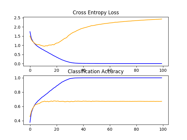
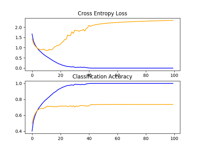
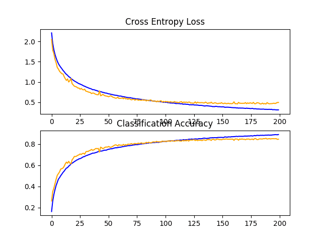
A figure is created and saved to file showing the learning curves of the model during training on the train and test dataset, both with regards to the loss and accuracy.
In this case, we can see that the model rapidly overfits the test dataset. This is clear if we look at the plot of loss (top plot), we can see that the model’s performance on the training dataset (blue) continues to improve whereas the performance on the test dataset (orange) improves, then starts to get worse at around 15 epochs.
Line Plots of Learning Curves for VGG 1 Baseline on the CIFAR-10 Dataset
Baseline: 2 VGG Blocks
The define_model() function for two VGG blocks is listed below.
Running the model in the test harness first prints the classification accuracy on the test dataset.
Note: Your results may vary given the stochastic nature of the algorithm or evaluation procedure, or differences in numerical precision. Consider running the example a few times and compare the average outcome.
In this case, we can see that the model with two blocks performs better than the model with a single block: a good sign.
1
> 71.080
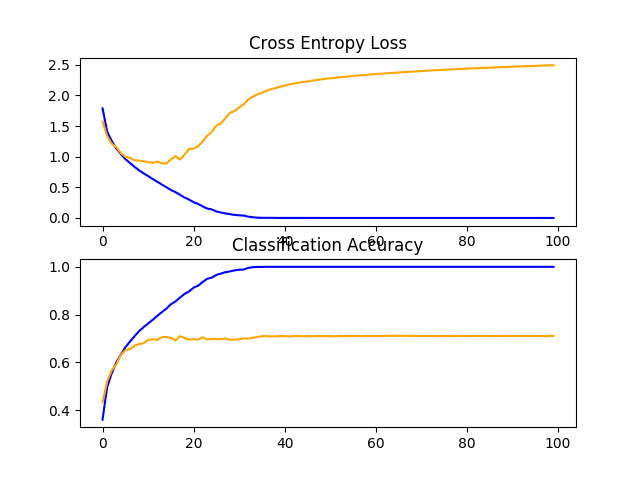
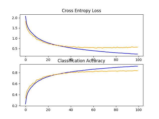
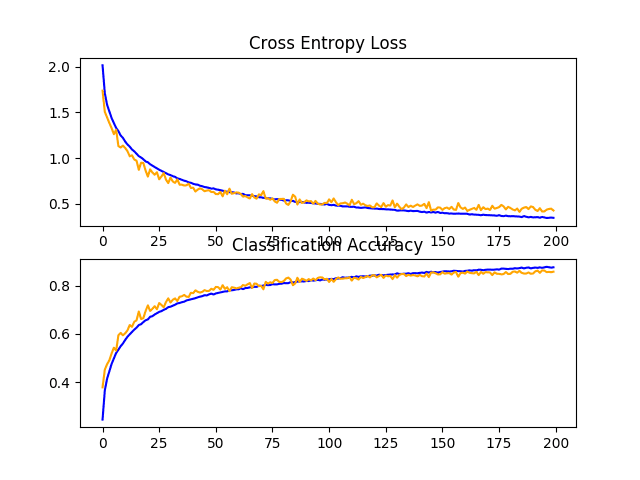
A figure showing learning curves is created and saved to file. In this case, we continue to see strong overfitting.
Line Plots of Learning Curves for VGG 2 Baseline on the CIFAR-10 Dataset
Baseline: 3 VGG Blocks
The define_model() function for three VGG blocks is listed below.
Running the model in the test harness first prints the classification accuracy on the test dataset.
Note: Your results may vary given the stochastic nature of the algorithm or evaluation procedure, or differences in numerical precision. Consider running the example a few times and compare the average outcome.
In this case, yet another modest increase in performance is seen as the depth of the model was increased.
1
> 73.500
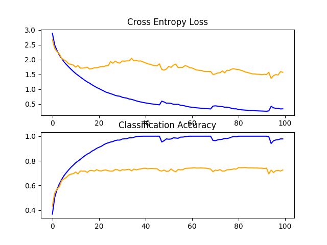
Reviewing the figures showing the learning curves, again we see dramatic overfitting within the first 20 training epochs.
Line Plots of Learning Curves for VGG 3 Baseline on the CIFAR-10 Dataset
Discussion
We have explored three different models with a VGG-based architecture.
The results can be summarized below, although we must assume some variance in these results given the stochastic nature of the algorithm:
VGG 1: 67.070%
VGG 2: 71.080%
VGG 3: 73.500%
In all cases, the model was able to learn the training dataset, showing an improvement on the training dataset that at least continued to 40 epochs, and perhaps more. This is a good sign, as it shows that the problem is learnable and that all three models have sufficient capacity to learn the problem.
The results of the model on the test dataset showed an improvement in classification accuracy with each increase in the depth of the model. It is possible that this trend would continue if models with four and five layers were evaluated, and this might make an interesting extension. Nevertheless, all three models showed the same pattern of dramatic overfitting at around 15-to-20 epochs.
These results suggest that the model with three VGG blocks is a good starting point or baseline model for our investigation.
The results also suggest that the model is in need of regularization to address the rapid overfitting of the test dataset. More generally, the results suggest that it may be useful to investigate techniques that slow down the convergence (rate of learning) of the model. This may include techniques such as data augmentation as well as learning rate schedules, changes to the batch size, and perhaps more.
In the next section, we will investigate some of these ideas for improving model performance.
How to Develop an Improved Model
Now that we have established a baseline model, the VGG architecture with three blocks, we can investigate modifications to the model and the training algorithm that seek to improve performance.
We will look at two main areas first to address the severe overfitting observed, namely regularization and data augmentation.
Regularization Techniques
There are many regularization techniques we could try, although the nature of the overfitting observed suggests that perhaps early stopping would not be appropriate and that techniques that slow down the rate of convergence might be useful.
We will look into the effect of both dropout and weight regularization or weight decay.
Dropout Regularization
Dropout is a simple technique that will randomly drop nodes out of the network. It has a regularizing effect as the remaining nodes must adapt to pick-up the slack of the removed nodes.
Dropout can be added to the model by adding new Dropout layers, where the amount of nodes removed is specified as a parameter. There are many patterns for adding Dropout to a model, in terms of where in the model to add the layers and how much dropout to use.
In this case, we will add Dropout layers after each max pooling layer and after the fully connected layer, and use a fixed dropout rate of 20% (e.g. retain 80% of the nodes).
The updated VGG 3 baseline model with dropout is listed below.
Running the model in the test harness prints the classification accuracy on the test dataset.
Note: Your results may vary given the stochastic nature of the algorithm or evaluation procedure, or differences in numerical precision. Consider running the example a few times and compare the average outcome.
In this case, we can see a jump in classification accuracy by about 10% from about 73% without dropout to about 83% with dropout.
1
> 83.450
Reviewing the learning curve for the model, we can see that overfitting has been addressed. The model converges well for about 40 or 50 epochs, at which point there is no further improvement on the test dataset.
This is a great result. We could elaborate upon this model and add early stopping with a patience of about 10 epochs to save a well-performing model on the test set during training at around the point that no further improvements are observed.
We could also try exploring a learning rate schedule that drops the learning rate after improvements on the test set stall.
Dropout has performed well, and we do not know that the chosen rate of 20% is the best. We could explore other dropout rates, as well as differing positioning of the dropout layers in the model architecture.
Line Plots of Learning Curves for Baseline Model With Dropout on the CIFAR-10 Dataset
Weight Decay
Weight regularization or weight decay involves updating the loss function to penalize the model in proportion to the size of the model weights.
This has a regularizing effect, as larger weights result in a more complex and less stable model, whereas smaller weights are often more stable and more general.
To learn more about weight regularization, see the post:
We can add weight regularization to the convolutional layers and the fully connected layers by defining the “kernel_regularizer” argument and specifying the type of regularization. In this case, we will use L2 weight regularization, the most common type used for neural networks and a sensible default weighting of 0.001.
The updated baseline model with weight decay is listed below.
Running the model in the test harness prints the classification accuracy of the test dataset.
Note: Your results may vary given the stochastic nature of the algorithm or evaluation procedure, or differences in numerical precision. Consider running the example a few times and compare the average outcome.
In this case, we see no improvement in the model performance on the test set; in fact, we see a small drop in performance from about 73% to about 72% classification accuracy.
1
> 72.550
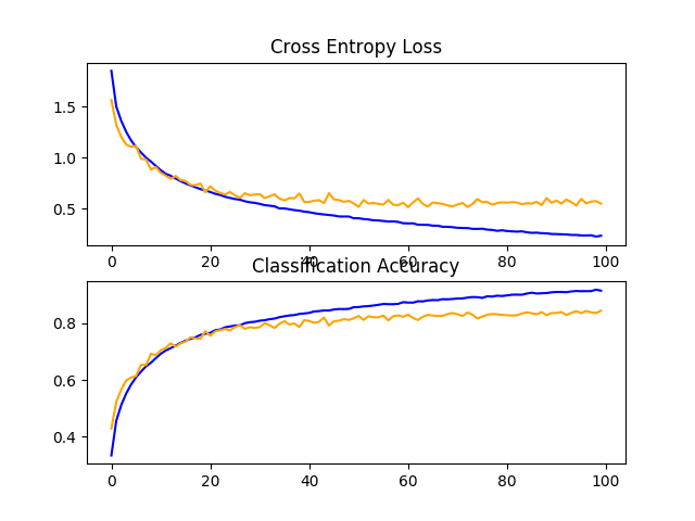
Reviewing the learning curves, we do see a small reduction in the overfitting, but the impact is not as effective as dropout.
We might be able to improve the effect of weight decay by perhaps using a larger weighting, such as 0.01 or even 0.1.
Line Plots of Learning Curves for Baseline Model With Weight Decay on the CIFAR-10 Dataset
Data Augmentation
Data augmentation involves making copies of the examples in the training dataset with small random modifications.
This has a regularizing effect as it both expands the training dataset and allows the model to learn the same general features, although in a more generalized manner.
There are many types of data augmentation that could be applied. Given that the dataset is comprised of small photos of objects, we do not want to use augmentation that distorts the images too much, so that useful features in the images can be preserved and used.
The types of random augmentations that could be useful include a horizontal flip, minor shifts of the image, and perhaps small zooming or cropping of the image.
We will investigate the effect of simple augmentation on the baseline image, specifically horizontal flips and 10% shifts in the height and width of the image.
Running the model in the test harness prints the classification accuracy on the test dataset.
Note: Your results may vary given the stochastic nature of the algorithm or evaluation procedure, or differences in numerical precision. Consider running the example a few times and compare the average outcome.
In this case, we see another large improvement in model performance, much like we saw with dropout. In this case, an improvement of about 11% from about 73% for the baseline model to about 84%.
1
> 84.470
Reviewing the learning curves, we see a similar improvement in model performances as we do with dropout, although the plot of loss suggests that model performance on the test set may have stalled slightly sooner than it did with dropout.
The results suggest that perhaps a configuration that used both dropout and data augmentation might be effective.
Line Plots of Learning Curves for Baseline Model With Data Augmentation on the CIFAR-10 Dataset
Discussion
In this section, we explored three approaches designed to slow down the convergence of the model.
A summary of the results is provided below:
Baseline + Dropout: 83.450%
Baseline + Weight Decay: 72.550%
Baseline + Data Augmentation: 84.470%
The results suggest that both dropout and data augmentation are having the desired effect, and weight decay, at least for the chosen configuration, did not.
Now that the model is learning well, we can look for both improvements on what is working, as well as combinations on what is working.
How to Develop Further Improvements
In the previous section, we discovered that dropout and data augmentation, when added to the baseline model, result in a model that learns the problem well.
We will now investigate refinements of these techniques to see if we can further improve the model’s performance. Specifically, we will look at a variation of dropout regularization and combining dropout with data augmentation.
Learning has slowed down, so we will investigate increasing the number of training epochs to give the model enough space, if needed, to expose the learning dynamics in the learning curves.
Variation of Dropout Regularization
Dropout is working very well, so it may be worth investigating variations of how dropout is applied to the model.
One variation that might be interesting is to increase the amount of dropout from 20% to 25% or 30%. Another variation that might be interesting is using a pattern of increasing dropout from 20% for the first block, 30% for the second block, and so on to 50% at the fully connected layer in the classifier part of the model.
This type of increasing dropout with the depth of the model is a common pattern. It is effective as it forces layers deep in the model to regularize more than layers closer to the input.
The baseline model with dropout updated to use a pattern of increasing dropout percentage with model depth is defined below.
Running the model in the test harness prints the classification accuracy on the test dataset.
Note: Your results may vary given the stochastic nature of the algorithm or evaluation procedure, or differences in numerical precision. Consider running the example a few times and compare the average outcome.
In this case, we can see a modest lift in performance from fixed dropout at about 83% to increasing dropout at about 84%.
1
> 84.690
Reviewing the learning curves, we can see that the model converges well, with performance on the test dataset perhaps stalling at around 110 to 125 epochs. Compared to the learning curves for fixed dropout, we can see that again the rate of learning has been further slowed, allowing further refinement of the model without overfitting.
This is a fruitful area for investigation on this model, and perhaps more dropout layers and/or more aggressive dropout may result in further improvements.
Line Plots of Learning Curves for Baseline Model With Increasing Dropout on the CIFAR-10 Dataset
Dropout and Data Augmentation
In the previous section, we discovered that both dropout and data augmentation resulted in a significant improvement in model performance.
In this section, we can experiment with combining both of these changes to the model to see if a further improvement can be achieved. Specifically, whether using both regularization techniques together results in better performance than either technique used alone.
The full code listing of a model with fixed dropout and data augmentation is provided below for completeness.
1
2
3
4
5
6
7
8
9
10
11
12
13
14
15
16
17
18
19
20
21
22
23
24
25
26
27
28
29
30
31
32
33
34
35
36
37
38
39
40
41
42
43
44
45
46
47
48
49
50
51
52
53
54
55
56
57
58
59
60
61
62
63
64
65
66
67
68
69
70
71
72
73
74
75
76
77
78
79
80
81
82
83
84
85
86
87
88
89
90
91
92
93
94
95
96
97
98
# baseline model with dropout and data augmentation on the cifar10 dataset
import sys
from matplotlib import pyplot
from keras.datasets import cifar10
from keras.utils import to_categorical
from keras.models import Sequential
from keras.layers import Conv2D
from keras.layers import MaxPooling2D
from keras.layers import Dense
from keras.layers import Flatten
from keras.optimizers import SGD
from keras.preprocessing.image import ImageDataGenerator
Running the model in the test harness prints the classification accuracy on the test dataset.
Note: Your results may vary given the stochastic nature of the algorithm or evaluation procedure, or differences in numerical precision. Consider running the example a few times and compare the average outcome.
In this case, we can see that as we would have hoped, using both regularization techniques together has resulted in a further lift in model performance on the test set. In this case, combining fixed dropout with about 83% and data augmentation with about 84% has resulted in an improvement to about 85% classification accuracy.
1
> 85.880
Reviewing the learning curves, we can see that the convergence behavior of the model is also better than either fixed dropout and data augmentation alone. Learning has been slowed without overfitting, allowing continued improvement.
The plot also suggests that learning may not have stalled and may have continued to improve if allowed to continue, but perhaps very modestly.
Results might be further improved if a pattern of increasing dropout was used instead of a fixed dropout rate throughout the depth of the model.
Line Plots of Learning Curves for Baseline Model With Dropout and Data Augmentation on the CIFAR-10 Dataset
Dropout and Data Augmentation and Batch Normalization
We can expand upon the previous example in a few ways.
First, we can increase the number of training epochs from 200 to 400, to give the model more of an opportunity to improve.
Next, we can add batch normalization in an effort to stabilize the learning and perhaps accelerate the learning process. To offset this acceleration, we can increase the regularization by changing the dropout from a fixed pattern to an increasing pattern.
The full code listing of a model with increasing dropout, data augmentation, batch normalization, and 400 training epochs is provided below for completeness.
1
2
3
4
5
6
7
8
9
10
11
12
13
14
15
16
17
18
19
20
21
22
23
24
25
26
27
28
29
30
31
32
33
34
35
36
37
38
39
40
41
42
43
44
45
46
47
48
49
50
51
52
53
54
55
56
57
58
59
60
61
62
63
64
65
66
67
68
69
70
71
72
73
74
75
76
77
78
79
80
81
82
83
84
85
86
87
88
89
90
91
92
93
94
95
96
97
98
99
100
101
102
103
104
105
106
# baseline model with dropout and data augmentation on the cifar10 dataset
import sys
from matplotlib import pyplot
from keras.datasets import cifar10
from keras.utils import to_categorical
from keras.models import Sequential
from keras.layers import Conv2D
from keras.layers import MaxPooling2D
from keras.layers import Dense
from keras.layers import Flatten
from keras.optimizers import SGD
from keras.preprocessing.image import ImageDataGenerator
Running the model in the test harness prints the classification accuracy on the test dataset.
Note: Your results may vary given the stochastic nature of the algorithm or evaluation procedure, or differences in numerical precision. Consider running the example a few times and compare the average outcome.
In this case, we can see that we achieved a further lift in model performance to about 88% accuracy, improving upon both dropout and data augmentation alone at about 84% and upon the increasing dropout alone at about 85%.
1
> 88.620
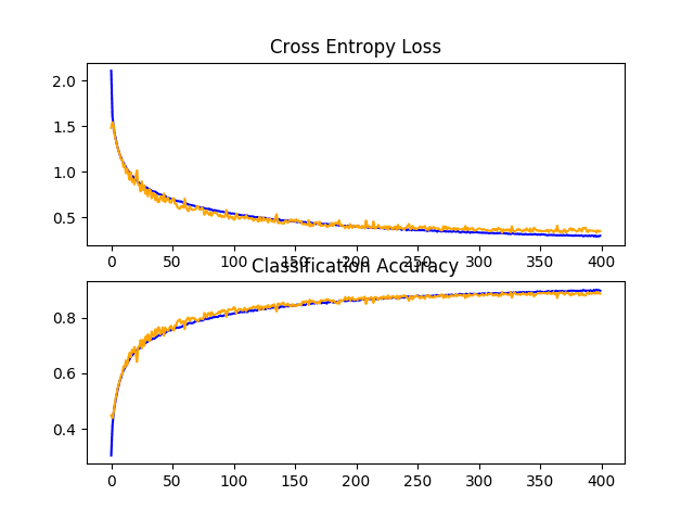
Reviewing the learning curves, we can see the training of the model shows continued improvement for nearly the duration of 400 epochs. We can see perhaps a slight drop-off on the test dataset at around 300 epochs, but the improvement trend does continue.
The model may benefit from further training epochs.
Line Plots of Learning Curves for Baseline Model With Increasing Dropout, Data Augmentation, and Batch Normalization on the CIFAR-10 Dataset
Discussion
In this section, we explored two approaches designed to expand upon changes to the model that we know already result in an improvement
The model is now learning well and we have good control over the rate of learning without overfitting.
We might be able to achieve further improvements with additional regularization. This could be achieved with more aggressive dropout in later layers. It is possible that further addition of weight decay may improve the model.
So far, we have not tuned the hyperparameters of the learning algorithm, such as the learning rate, which is perhaps the most important hyperparameter. We may expect further improvements with adaptive changes to the learning rate, such as use of an adaptive learning rate technique such as Adam. These types of changes may help to refine the model once converged.
How to Finalize the Model and Make Predictions
The process of model improvement may continue for as long as we have ideas and the time and resources to test them out.
At some point, a final model configuration must be chosen and adopted. In this case, we will keep things simple and use the baseline model (VGG with 3 blocks) as the final model.
First, we will finalize our model by fitting a model on the entire training dataset and saving the model to file for later use. We will then load the model and evaluate its performance on the hold out test dataset, to get an idea of how well the chosen model actually performs in practice. Finally, we will use the saved model to make a prediction on a single image.
Save Final Model
A final model is typically fit on all available data, such as the combination of all train and test dataset.
In this tutorial, we will demonstrate the final model fit only on the just training dataset to keep the example simple.
The first step is to fit the final model on the entire training dataset.
After running this example you will now have a 4.3-megabyte file with the name ‘final_model.h5‘ in your current working directory.
Evaluate Final Model
We can now load the final model and evaluate it on the hold out test dataset.
This is something we might do if we were interested in presenting the performance of the chosen model to project stakeholders.
The test dataset was used in the evaluation and choosing among candidate models. As such, it would not make a good final test hold out dataset. Nevertheless, we will use it as a hold out dataset in this case.
The model can be loaded via the load_model() function.
The complete example of loading the saved model and evaluating it on the test dataset is listed below.
1
2
3
4
5
6
7
8
9
10
11
12
13
14
15
16
17
18
19
20
21
22
23
24
25
26
27
28
29
30
31
32
33
34
35
36
37
38
39
# evaluate the deep model on the test dataset
from keras.datasets import cifar10
from keras.models import load_model
from keras.utils import to_categorical
# load train and test dataset
def load_dataset():
# load dataset
(trainX,trainY),(testX,testY)=cifar10.load_data()
# one hot encode target values
trainY=to_categorical(trainY)
testY=to_categorical(testY)
returntrainX,trainY,testX,testY
# scale pixels
def prep_pixels(train,test):
# convert from integers to floats
train_norm=train.astype('float32')
test_norm=test.astype('float32')
# normalize to range 0-1
train_norm=train_norm/255.0
test_norm=test_norm/255.0
# return normalized images
returntrain_norm,test_norm
# run the test harness for evaluating a model
def run_test_harness():
# load dataset
trainX,trainY,testX,testY=load_dataset()
# prepare pixel data
trainX,testX=prep_pixels(trainX,testX)
# load model
model=load_model('final_model.h5')
# evaluate model on test dataset
_,acc=model.evaluate(testX,testY,verbose=0)
print('> %.3f'%(acc *100.0))
# entry point, run the test harness
run_test_harness()
Running the example loads the saved model and evaluates the model on the hold out test dataset.
The classification accuracy for the model on the test dataset is calculated and printed.
Note: Your results may vary given the stochastic nature of the algorithm or evaluation procedure, or differences in numerical precision. Consider running the example a few times and compare the average outcome.
In this case, we can see that the model achieved an accuracy of about 73%, very close to what we saw when we evaluated the model as part of our test harness.
1
73.750
Make Prediction
We can use our saved model to make a prediction on new images.
The model assumes that new images are color, they have been segmented so that one image contains one centered object, and the size of the image is square with the size 32×32 pixels.
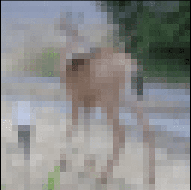
Below is an image extracted from the CIFAR-10 test dataset. You can save it in your current working directory with the filename ‘sample_image.png‘.
We will pretend this is an entirely new and unseen image, prepared in the required way, and see how we might use our saved model to predict the integer that the image represents.
For this example, we expect class “4” for “Deer“.
First, we can load the image and force it to the size to be 32×32 pixels. The loaded image can then be resized to have a single channel and represent a single sample in a dataset. The load_image() function implements this and will return the loaded image ready for classification.
Importantly, the pixel values are prepared in the same way as the pixel values were prepared for the training dataset when fitting the final model, in this case, normalized.
1
2
3
4
5
6
7
8
9
10
11
12
# load and prepare the image
def load_image(filename):
# load the image
img=load_img(filename,target_size=(32,32))
# convert to array
img=img_to_array(img)
# reshape into a single sample with 3 channels
img=img.reshape(1,32,32,3)
# prepare pixel data
img=img.astype('float32')
img=img/255.0
returnimg
Next, we can load the model as in the previous section and call the predict_classes() function to predict the object in the image.
1
2
# predict the class
result=model.predict_classes(img)
The complete example is listed below.
1
2
3
4
5
6
7
8
9
10
11
12
13
14
15
16
17
18
19
20
21
22
23
24
25
26
27
28
29
30
# make a prediction for a new image.
from keras.preprocessing.image import load_img
from keras.preprocessing.image import img_to_array
from keras.models import load_model
# load and prepare the image
def load_image(filename):
# load the image
img=load_img(filename,target_size=(32,32))
# convert to array
img=img_to_array(img)
# reshape into a single sample with 3 channels
img=img.reshape(1,32,32,3)
# prepare pixel data
img=img.astype('float32')
img=img/255.0
returnimg
# load an image and predict the class
def run_example():
# load the image
img=load_image('sample_image.png')
# load model
model=load_model('final_model.h5')
# predict the class
result=model.predict_classes(img)
print(result[0])
# entry point, run the example
run_example()
Running the example first loads and prepares the image, loads the model, and then correctly predicts that the loaded image represents a ‘deer‘ or class ‘4‘.
1
4
Extensions
This section lists some ideas for extending the tutorial that you may wish to explore.
Pixel Scaling. Explore alternate techniques for scaling the pixels, such as centering and standardization, and compare performance.
Learning Rates. Explore alternate learning rates, adaptive learning rates, and learning rate schedules and compare performance.
Transfer Learning. Explore using transfer learning, such as a pre-trained VGG-16 model on this dataset.
If you explore any of these extensions, I’d love to know.
Post your findings in the comments below.
Further Reading
This section provides more resources on the topic if you are looking to go deeper.
It provides self-study tutorials on topics like: classification, object detection (yolo and rcnn), face recognition (vggface and facenet), data preparation and much more...
Finally Bring Deep Learning to your Vision Projects
Thanks for the post. Would be interesting to see how your training time and performance change if you switched optimizers to Adam and CyclicLR. Thanks!
Maybe the first thing that should be taught about neural networks is the weighted sum as a linear associative memory. In a general way because there are provisos.
In the case there are more weights than patterns to learn you get error correction and a neuron can be defined as a branching process. https://discourse.numenta.org/t/towards-demystifying-over-parameterization-in-deep-learning/5985
This was known in early literature on the subject. Has it been somewhat forgotten?
This is a great tutorial ever! Can you please help me how can I load my own collected data set. I structured my data with the following code for my data sets.
When i replaced this (trainX, trainY), (testX, testY) = cifar10.load_data() by this (trainX, trainY), (testX, testY) = (train_it , test_it ). I get the following error
~\.conda\envs\tensorflow\lib\urllib\request.py in _open(self, req, data)
543 result = self._call_chain(self.handle_open, protocol, protocol +
–> 544 ‘_open’, req)
545 if result:
~\.conda\envs\tensorflow\lib\urllib\request.py in _call_chain(self, chain, kind, meth_name, *args)
503 func = getattr(handler, meth_name)
–> 504 result = func(*args)
505 if result is not None:
Exception: URL fetch failure on https://www.cs.toronto.edu/~kriz/cifar-10-python.tar.gz: None — [WinError 10060] A connection attempt failed because the connected party did not properly respond after a period of time, or established connection failed because connected host has failed to respond
your code (below) leaves no output in Jupyter Notebook, it’s as though nothing runs. Running the same code in Spyder throws up lot’s of errors. Can you please help me with this because i want to work through the following examples relating to modification of the training model supplied on thor web based examples page.
thanks in advance.
# test harness for evaluating models on the cifar10 dataset
import sys
from matplotlib import pyplot
from keras.datasets import cifar10
from keras.utils import to_categorical
from keras.models import Sequential
from keras.layers import Conv2D
from keras.layers import MaxPooling2D
from keras.layers import Dense
from keras.layers import Flatten
from keras.optimizers import SGD
from keras.utils import np_utils
import tensorflow as ts
# load train and test dataset
def load_dataset():
# load dataset
(trainX, trainY), (testX, testY) = cifar10.load_data()
# one hot encode target values
trainY = to_categorical(trainY)
testY = to_categorical(testY)
return trainX, trainY, testX, testY
# scale pixels
def prep_pixels(train, test):
# convert from integers to floats
train_norm = train.astype(‘float32’)
test_norm = test.astype(‘float32′)
# normalize to range 0-1
train_norm = train_norm / 255.0
test_norm = test_norm / 255.0
# return normalized images
return train_norm, test_norm
# define cnn model
def define_model():
model = Sequential()
model.add(Conv2D(32, (3, 3), activation=’relu’, kernel_initializer=’he_uniform’, padding=’same’, input_shape=(32, 32, 3)))
model.add(Conv2D(32, (3, 3), activation=’relu’, kernel_initializer=’he_uniform’, padding=’same’))
model.add(MaxPooling2D((2, 2)))
model.add(Conv2D(64, (3, 3), activation=’relu’, kernel_initializer=’he_uniform’, padding=’same’))
model.add(Conv2D(64, (3, 3), activation=’relu’, kernel_initializer=’he_uniform’, padding=’same’))
model.add(MaxPooling2D((2, 2)))
model.add(Conv2D(128, (3, 3), activation=’relu’, kernel_initializer=’he_uniform’, padding=’same’))
model.add(Conv2D(128, (3, 3), activation=’relu’, kernel_initializer=’he_uniform’, padding=’same’))
model.add(MaxPooling2D((2, 2)))
# Output part
# example output part of the model
model.add(Flatten())
model.add(Dense(128, activation=’relu’, kernel_initializer=’he_uniform’))
model.add(Dense(10, activation=’softmax’))
# compile model
opt = SGD(lr=0.001, momentum=0.9)
model.compile(optimizer=opt, loss=’categorical_crossentropy’, metrics=[‘accuracy’])
return model
thank you for your reply and your web page. i also discovered that the issue was my fault. when i stuck paraters such as into model.fit.generator (…,…,epochs=1,…, verbose=1) i discovered the model would take over 70 hours to run with epochs = 400. amazing what a it of output (from verbose=1) tells you!
I have one final Question. If you look at https://en.wikipedia.org/wiki/CIFAR-10 you will see 14 references published over 8 years that reduce the uncertainty on test set visualization assurity from 21.1% down to 1% on CIFAR-10 datasets. I have started to look at these papers and find most technicaly overwhelming. Some provide Github source links, most do not. You as a much more seasoned practitioner than I, I was wondering what is your feelings about the direction and eventual outcome of these rather detailed expositions? I wonder about if there will be a algorithmic breakthrough in NN formulation and if so given the pace of competition the means of arriving at a optimal outcome (along with commercial return considerations) will means to get to such optimal outcomes makes the means to the end proprietry and no longer library accessible open source material? Thanks for your post with heartfelt thanks.
The pattern I see is that amazing breakthroughs come from complex bespoke methods, then some clever kid figure out a simpler and more general method to do the same thing that becomes the new norm – and put into a library/tool. Repeat.
A deep and very extensive lesson on image multi-class classification..
The 400 epochs takes my mac pro i7 (6 cores) 16 hours of running.
Happily I saved the trained model on “h5 file format”, and I load the model and I re-run another 100 extra epochs and I got an Accuracy of 88.570 (close to your 88.6%) , but I apply not only your 3 recommended regularizers altogether ( dropout + batchnormalization + data_augmentation ) but also the weight decay (l2) with the 3 CNN VGG blocks.
So it does not get more accuracy to add kernel_regularizer to the 3 previous one regularizers and even training for another 100 extra epochs …
I see on my last training history plot, the last 100 epochs of 500 total, some instability on test (but no on train data) performance (some kind of quick fluctuations of more than 10% variation on Acc or loss but at the end it is stabilized around 88%.
it means to me an asymptotic approach under this parameters selection: l2, dropout variable, SGD, data-agumentation distortion , batchnormalization !!
I do not expect so much improvement changing to Adam optimizer, or l1-l2 weight regularizers, …but for sure if I increase the numbers of VGG blocks…
Anyway, I will like to try to apply a Transfer Learning improvement method using VVG16 (without top layers) and my own dense layers classifier trained on top … I will report it if I get something
I am a little confused about the interpretation of my results but, I share here:
1) When I used your model “VGG3” with increased dropout rate + data augmentation + batch normalization, including batchnormalization, dropout and l1-l2weight decay, I get same results as yours around 88% accuracy, It takes more than 16 hours of cpu, BUT
2) when using VGG16 without his top as Transfer Learning to our head and, with your data_aumentation profile and the own preprocess_input of VGG16 and, I train the whole model (VGG16 weight frozen model + our head), Ok I reduce cpu time to 2.5 hours but I get a ridiculous 63.6 % accuracy … I do not understand it…
3) Ok when I got the outputs of VGG16 frozen model (without top) once (same data_augmentation and data preprocessing)… as new inputs of our head model ok, I reduce now the cpu time to 2 minutes (vs 2.5 hour before due to the fact I do not pass every time the input through the frozen VGG16 model but only first time and I save them), but still the accuracy is around 64%, so I still do not understand how is it possible? if VGG16 trained model is much better than the propose here VGG3…
4) I know I am applying well the VGG16 model because, when I defrost the last Block number 5 of VGG16 (as proposed by F. Chollet in his post) I start getting better results (81 % accuracy for only 50 epochs vs 88% of 400 epochs it seem reasonable), but now the cpu time climb up to 2.5 hours
5) When I re-train the model (when previous weights saved on item 4) I got 82.3% accuracy for only 50 epochs more…
So I think if I defrost the VGG16 (transfer learning) block 5 (as a way to retrain the model with our own CIFAR dataset) I start getting the expected results path … but using VGG16 alone frozen weights and injecting his output to our head model …does not crus the problem in terms of accuracy and cpu time as expected…so I am little confused about this expected transfer Learning behaviour (without the needs of defrost any inside blocks) …(!)
Very useful tutorial! Oddly, I was unable to replicate your accuracy rates of 83% and 84% when employing augmentation and dropout, flattening off right at 80% when using both, despire having copied the architecture and data loaders practically line for line into Colab with Keras.
For anyone interested, I obtained my best results when using increasing dropout, data augmentation, the Nadam optimization algorithm, and an internal Keras function which allows you to decrease the learning rate when you reach a validation loss plateau. Specifically, the code is:
callbacks_list = [tf.keras.callbacks.ReduceLROnPlateau(monitor=”val_loss”, factor=0.5, patience=5)]
Insert the following into the history.fit command:
callbacks=callbacks_list
This method has consistently reached 82% after 100 epochs, with very little overfitting. Presumably extending the number of epochs is the way to go, and so I’m hoping to reach 88% or higher in the next couple days by tweaking this.
Pardon the verbose reply.
Thanks for making this, Jason! It’s been extremely useful to me!
i have used prediction on image classification for 4 classes but it gives only two values when i print result value it gives 2 and 3 not 0 and 1 what is the mistake
import sys
import os
from keras.preprocessing.image import ImageDataGenerator
from keras import optimizers
from keras.models import Sequential
from keras.layers import Dropout, Flatten, Dense, Activation
from keras.layers import Conv2D, MaxPooling2D
from keras import callbacks
target_dir = ‘/content/gdrive/My Drive/’
if not os.path.exists(target_dir):
os.mkdir(target_dir)
model.save(‘/content/gdrive/My Drive/modelnew.h5’)
model.save_weights(‘/content/gdrive/My Drive/weights1.h5’)
#Calculate execution time
end = time.time()
dur = end-start
if dur60 and dur<3600:
dur=dur/60
print("Execution Time:",dur,"minutes")
else:
dur=dur/(60*60)
print("Execution Time:",dur,"hours")
—–
import os
import numpy as np
from keras.preprocessing.image import ImageDataGenerator, load_img, img_to_array
from keras.models import Sequential, load_model
import time
#Prediction Function
def predict(file):
x = load_img(file, target_size=(img_width,img_height))
x = img_to_array(x)
x = np.expand_dims(x, axis=0)
array = model.predict(x)
result = array[0]
print(result)
answer = np.argmax(result)
print(answer)
if answer == 0:
print("Predicted:MildDemented")
elif answer == 1:
print("Predicted:VeryDemented")
elif answer == 2:
print("Predicted: nonDemented")
return answer
#Walk the directory for every image
for i, ret in enumerate(os.walk(test_path)):
for i, filename in enumerate(ret[2]):
if filename.startswith("."):
continue
Another awesome and illuminating case study.
However I can’t find a way to suppress the massive print output from the load_dataset.
This generic problem is also unanswered on stackoverflow. (verbose=0) doesn’t work.
Hate to bother you with something so trivial, but – any idea?
All of these libs (keras, tf, sklearn) “spew” to stdout or stder. If I wrote code that did that in industry, there would have all kinds of hell to pay.
Thanks a lot for these types of posts they have helped me in building up the basics of my Machine Learning and Deep Learning journey.
Can you kindly clear a doubt of mine that our model is very robust because of the Conv2D layers we have added, but we did not add a single Dropout Layer in the Model. So by this approach, will our model might suffer from over-fitting?
can you pls give me a code to import the dataset on the drive(i,e:.dataset stored in c drive) to jupyter notebook rather importing from keras or tensorflow to jupyter notebook?
I could execute the command on a different computer and store (somehow) in a binary file and transfer to the “Firewalled” computer to permit something like “(trainX, trainY), (testX, testY) = ”
I’m blanking on the details how to store and retrieve the content of a local “cifar10” file.
Thanks for this valuable post. Do you know any paper that implements cifar10 with vgg16 (until block3 like mentioned on this page) and get the same accuracy? I had implemented it and get an accuracy of 83.25! Now I want to add this to my paper and I need a published reference.
I achieved 90.09% accuracy in 300 epochs with the slight modification – 1st CNN block is 48 (instead of 32). 2nd and 3rd left untouched. Why do we have to duplicate filters every block?
hi
im new in python and deep learning but for my university final exam i need running and ofcurse learning a sampe deep learning process on some image data.im using Google Colab and ran your code(bellow) but it just keeps running with no result . i think maybe the dataset loading is taking so long.so first question is that am i correctly running this code? ( i have not downloaded the dataset and loading in online as your code does it)
this code(your code) making final_model.h5 and it takes too long(maybe im wrong)
so if please help me to run full code simply (just copy and paste) to make models and then rerun saved model on my own image and get the output
thank you. Im really noob so please forgive me .
—————————————————————
import sys
from matplotlib import pyplot
from keras.datasets import cifar10
from keras.utils import to_categorical
from keras.models import Sequential
from keras.layers import Conv2D
from keras.layers import MaxPooling2D
from keras.layers import Dense
from keras.layers import Flatten
from keras.layers import Dropout
from keras.optimizers import SGD
# load train and test dataset
def load_dataset():
# load dataset
(trainX, trainY), (testX, testY) = cifar10.load_data()
# one hot encode target values
trainY = to_categorical(trainY)
testY = to_categorical(testY)
return trainX, trainY, testX, testY
# scale pixels
def prep_pixels(train, test):
# convert from integers to floats
train_norm = train.astype(‘float32’)
test_norm = test.astype(‘float32′)
# normalize to range 0-1
train_norm = train_norm / 255.0
test_norm = test_norm / 255.0
# return normalized images
return train_norm, test_norm
# run the test harness for evaluating a model
def run_test_harness_save():
# load dataset
trainX, trainY, testX, testY = load_dataset()
# prepare pixel data
trainX, testX = prep_pixels(trainX, testX)
# define model
model = define_model()
# fit model
model.fit(trainX, trainY, epochs=1, batch_size=1, verbose=0)
# save model
model.save(‘final_model.h5’)
# run the test harness for evaluating a model
———————————————————————
hi again
I treid a lot finaly could run it
for fast answer I tested it in echo 1 and it worked( of course gave wrong answers)
then I set echo on 100 and ran it again . untill now its been 7 hours its running!
im working with google colab so i dont think the hw is problem
is that normal ?!
second question is that how can i get answer like ‘dog’, ‘cat’ ,.. instead of number ?
after almost 8 hours saved the model )
accuracy more than 80%
but still i donno these numbers
for car i get 5 and …
how can i get name of object(cat or car …) instead of number ?
I have a perhaps dumb (and definitely newbie) question:
What is the reasoning, aside from empirically proven good prediction performance, behind the choice of 128 units in the Dense layer right after flattening? The value 128 remains unchanged regardless of whether 1, 2, or 3 blocks are used.
I understand that the second Dense layer outputs 10 because of the 10 classes, but don’t get the 128 in the layer before.
I tried your model architecture with data augmentation, varying dropout, batch normalization. but the accuracy is not improving above 65%. can you suggest how to improve this.
My training code:
import os
import tensorflow as tf
from tensorflow import keras
from keras.preprocessing.image import ImageDataGenerator
from tensorflow.keras.models import Sequential
#from tensorflow.keras.layers import Dense, Conv2D, MaxPooling2D, Flatten
from keras.layers.convolutional import Convolution2D
from keras.layers import Dense
from keras.layers.convolutional import MaxPooling2D
from keras.layers import Flatten
from keras.layers import Dropout
from keras.layers import BatchNormalization
from keras.optimizers import SGD
My testing code:
import numpy as np
import tensorflow as tf
from keras.preprocessing.image import ImageDataGenerator
from keras.preprocessing import image
from keras.models import load_model
from sklearn.metrics import confusion_matrix, accuracy_score
import matplotlib.pyplot as plt
import cv2
validation_generator.reset()
pred= model.predict_generator(validation_generator, nb_samples,verbose=1)
predicted_class_indices=np.argmax(pred,axis=1)
labels=validation_generator.class_indices
for i in labels:
print(labels[i])
labels2=dict((v,k) for k,v in labels.items())
predictions=[labels2[k] for k in predicted_class_indices]
print(“prediction class are : “, predicted_class_indices)
print(“labels are : “, labels)
print(“predictions: “, predictions[:5])
i train my model with 40 epoch, but when i try predict with some image, the result is equal to 4 for all image, what wrong with my model, plese help me
Thanks for the reply.
I tried without one-hot-encoding the target variable . And I was able to predict the probabilities of each class for the test images. Based on it , I have predicted the class as shown below
For e.g
probability_model = tf.keras.Sequential([model,
tf.keras.layers.Softmax()])
predictions = probability_model.predict(test_images)
print(predictions.shape)
print(predictions[0])
## based on the max value of probability , predict the class.
test_predicted_labels = []
for i in range(len(predictions)):
pred_label = np.argmax(predictions[i])
test_predicted_labels.append(pred_label)
This is the output.
—————–
(10000, 10)
[0.08861145 0.08834625 0.08928947 0.1760501 0.08857722 0.10344525
0.08981362 0.08847508 0.09888937 0.08850213]
Using the test_predicted_labels above , I have printed the classification report.
Am I missing something ? What benefit would hot encoding the target give ?
Thanks for these amazing suggestions on baseline model improvement. I reached out to ask if using test data as the validation data for model training can lead to data leakage.
Just one question.
Instead of one hot encoding target variable, you could have used sparse_categorical_crossentropy loss. Is there a specific reason that you didn’t follow this approach?
Very nice tutorial, I have some comments to improve it if you don’t mind:
1. Using plain code instead of functions as in [1],[2]. This helps to clarify stuff for beginners and make it easier to port the code to another tool e.g. PyTorch.
2. add notebook version e.g. google colab to run the code and test it, this helps to avoid debugging or answering debug questions (I already created a colab notebook and I can share it with you if you like).
3. maybe use the same tutorial as a base to another tutorial that explains more about different training curves, what they mean, and how to modify the model to get better performance.
thankyou very much sir……i have started my machine learning journey by following your MACHINE LEARNING MASTERY
if possible could be please make a tutorial on predicting drug-disease associations using deep learning
Hi, I’ve made a novel architecture with just 2M parameters and without any extra data augmentation on CIFAR-10 and got 98.88% accuracy on training dataset and 74.0% accuracy on validation dataset after 100 epochs. Do you think it’s worth to work on that any further?
Hi Jason very good work! Can I apply the same techniques (dropout, data augmentation, batch normalization) to MLP networks? What do you suggest for MLP architectures for Cifar10 dataset?
Hi, very good work! Can I apply the same techniques (dropout, data augmentation, batch normalization) to MLP networks? What do you suggest for MLP architectures especially for Cifar10 dataset?
Hi. Thank for your site. I trained my network and got 88% accuracy. Then, when I run prediction, output of my network only detect deer. Are you check other pictures and see your network’s answer?
this code leaves :
import matplotlib.pyplot as plt
from tensorflow.keras.layers import Input, Conv2D, Dense, Flatten, Dropout
from tensorflow.keras.layers import GlobalMaxPooling2D, MaxPooling2D
from tensorflow.keras.layers import BatchNormalization
from tensorflow.keras.models import Model
this error:
from tensorflow.keras.layers import Input, Conv2D, Dense, Flatten, Dropout
ModuleNotFoundError: No module named ‘tensorflow.keras’
but when i do try installing it using
pip install tensorflow.keras
it gives another error
ERROR: Could not find a version that satisfies the requirement tensorflow.keras (from versions: none)
ERROR: No matching distribution found for tensorflow.keras
Hi John…There are many ways such as the following:
To establish the accuracy of a CNN (Convolutional Neural Network) classifier from multiple executions, you can follow these steps:
1. **Cross-Validation**: Perform cross-validation, commonly using K-fold cross-validation, to train and test your model on different subsets of your dataset. This helps ensure that the model performs well across various unseen data samples.
2. **Repeat Runs**: Train and test the CNN multiple times (repeated runs) to average out the variability caused by different initializations of weights or partitioning of data.
3. **Record Metrics**: Each time you run the model, record key performance metrics such as accuracy, precision, recall, and F1-score. These metrics will give a comprehensive view of performance.
4. **Average Results**: Calculate the mean and standard deviation of these metrics across all runs to assess the overall performance and stability of your model.
5. **Confidence Intervals**: Establish confidence intervals for your accuracy estimates to understand the range in which the true accuracy of your model likely falls.
By following these steps, you can reliably estimate the accuracy and robustness of your CNN classifier, ensuring it performs consistently across different sets of data and initialization conditions.
Thank you for yout answer.
I would like to know how did you compute it because I am trying to replicate the accuracy results of the tutorial. For example when in the second baseline model you state you got 71.080 accuracy. How that 71.080 was computed?
Thank you in advance for your answer


Throwing error train not defined. Any suggestion to solve this problem?
I have some suggestions here that may help:
https://machinelearningmastery.com/faq/single-faq/why-does-the-code-in-the-tutorial-not-work-for-me
Sorry, but if you’re using all these Keras libraries, you probably shouldn’t use the term “from scratch”. That’s false advertising.
From scratch here means, not using a pre-trained model or transfer learning, but training the model weights from random (scratch) to a viable model.
Thanks for the post. Would be interesting to see how your training time and performance change if you switched optimizers to Adam and CyclicLR. Thanks!
Great suggestion!
good morning sir.
thank you for posting emails to me.
It’s really excellent work what you have done.
could you help me regarding training segmentation models (from scratch) using CNN on BRATS Database?
please post me emails regarding the same.
thank you so much, sir.
I have some examples of Mask R-CNN for image segmentation in this book that may be a helpful start:
https://machinelearningmastery.com/deep-learning-for-computer-vision/
Please these questions for me.
What is epoch?
How can i transform 3D image to 2D.
How is weight and bias applied?
Thanks
This explains what an epoch is:
https://machinelearningmastery.com/faq/single-faq/what-is-the-difference-between-a-batch-and-an-epoch
Sorry, I don’t know about a “3d image”.
Weight and biases are inside the layers and are updated by training the model.
Maybe the first thing that should be taught about neural networks is the weighted sum as a linear associative memory. In a general way because there are provisos.
In the case there are more weights than patterns to learn you get error correction and a neuron can be defined as a branching process.
https://discourse.numenta.org/t/towards-demystifying-over-parameterization-in-deep-learning/5985
This was known in early literature on the subject. Has it been somewhat forgotten?
Thanks Sean.
# convert from integers to floats
train_norm = train.astype(‘float32’)
test_norm = test.astype(‘float32’)
# normalize to range 0-1
train_norm = train_norm / 255.0
test_norm = test_norm / 255.0
when running this code getting an error.
NameError: name ‘train’ is not defined.
could you please help to solve this sir.?
I have some suggestions here:
https://machinelearningmastery.com/faq/single-faq/why-does-the-code-in-the-tutorial-not-work-for-me
This is a great tutorial ever! Can you please help me how can I load my own collected data set. I structured my data with the following code for my data sets.
for file in listdir(folder):
# determine class
output = 0.0
if file.startswith(‘G’):
output = 1.0
elif file.startswith(‘M’):
output = 2.0
elif file.startswith(‘C’):
output = 4.0
elif file.startswith(‘S’):
output = 5.0
elif file.startswith(‘G1’):
output = 6.0
elif file.startswith(‘R’):
output = 7.0
# load image
photo = load_img(folder + file, target_size=(200, 200))
# convert to numpy array
photo = img_to_array(photo)
# store
photos.append(photo)
labels.append(output)
labeldirs = [‘G/’, ‘M/’, ‘C/’, ‘S/’, ‘G1/’, ‘R/’]
for labldir in labeldirs:
newdir = dataset_home + subdir + labldir
makedirs(newdir, exist_ok=True)
src_directory = ‘test/’
for file in listdir(src_directory):
src = src_directory + ‘/’ + file
dst_dir = ‘train/’
if random() < val_ratio:
dst_dir = 'test/'
if file.startswith('G'):
dst = dataset_home + dst_dir + 'G/' + file
copyfile(src, dst)
elif file.startswith('M'):
dst = dataset_home + dst_dir + 'M/' + file
copyfile(src, dst)
elif file.startswith('G1'):
dst = dataset_home + dst_dir + 'G1/' + file
copyfile(src, dst)
elif file.startswith('R'):
dst = dataset_home + dst_dir + 'R/' + file
copyfile(src, dst)
elif file.startswith('C'):
dst = dataset_home + dst_dir + 'C/' + file
copyfile(src, dst)
elif file.startswith('S'):
dst = dataset_home + dst_dir + 'S/' + file
copyfile(src, dst)
How can I load and use this structure of data set for this tutorial as this tutorial used the Keras API to just load the dataset as :
def load_dataset():
# load dataset
(trainX, trainY), (testX, testY) = cifar10.load_data()
# one hot encode target values
trainY = to_categorical(trainY)
testY = to_categorical(testY)
return trainX, trainY, testX, testY
Please help?
Thanks!
Maybe this tutorial will help you to load your dataset:
https://machinelearningmastery.com/how-to-load-large-datasets-from-directories-for-deep-learning-with-keras/
Thanks, I have loaded it as suggested in :
https://machinelearningmastery.com/how-to-load-large-datasets-from-directories-for-deep-learning-with-keras/
But how to proceed further with the structure of this tutorial.
I used image data generator and now I prepared the iterators as train_it and test_it can u guide how I used this further for the following function.
def load_dataset():
# load dataset
(trainX, trainY), (testX, testY) = cifar10.load_data()
# one hot encode target values
trainY = to_categorical(trainY)
testY = to_categorical(testY)
return trainX, trainY, testX, testY
is the statement (trainX, trainY), (testX, testY) = train_it ok?
Thanks!
Sorry, I don’t follow. What problem are you having exactly?
Thanks!
I have loaded data set successfully as given in :
https://machinelearningmastery.com/how-to-load-large-datasets-from-directories-for-deep-learning-with-keras/
I used image data generator and create an iterator for train_it and test_it.
Could you please elaborate on how I can use train_it and test_it in the following code by this tutorial.
def load_dataset():
# load dataset
(trainX, trainY), (testX, testY) = cifar10.load_data()
# one hot encode target values
trainY = to_categorical(trainY)
testY = to_categorical(testY)
return trainX, trainY, testX, testY
When i replaced this (trainX, trainY), (testX, testY) = cifar10.load_data() by this (trainX, trainY), (testX, testY) = (train_it , test_it ). I get the following error
Load-Prepare Memory error.
Any help would be appreciated.
The idea of using an ImageDataGenerator is that it does not load all of the data into memory, instead it loads one batch of images at a time.
Perhaps see an example of its usage in this tutorial:
https://machinelearningmastery.com/how-to-develop-a-convolutional-neural-network-to-classify-photos-of-dogs-and-cats/
Sir while loading the dataset I’m getting this erro
~\.conda\envs\tensorflow\lib\urllib\request.py in open(self, fullurl, data, timeout)
525
–> 526 response = self._open(req, data)
527
~\.conda\envs\tensorflow\lib\urllib\request.py in _open(self, req, data)
543 result = self._call_chain(self.handle_open, protocol, protocol +
–> 544 ‘_open’, req)
545 if result:
~\.conda\envs\tensorflow\lib\urllib\request.py in _call_chain(self, chain, kind, meth_name, *args)
503 func = getattr(handler, meth_name)
–> 504 result = func(*args)
505 if result is not None:
~\.conda\envs\tensorflow\lib\urllib\request.py in https_open(self, req)
1360 return self.do_open(http.client.HTTPSConnection, req,
-> 1361 context=self._context, check_hostname=self._check_hostname)
1362
~\.conda\envs\tensorflow\lib\urllib\request.py in do_open(self, http_class, req, **http_conn_args)
1319 except OSError as err: # timeout error
-> 1320 raise URLError(err)
1321 r = h.getresponse()
URLError:
During handling of the above exception, another exception occurred:
Exception Traceback (most recent call last)
in
7 print(‘> %.3f’ % (acc * 100.0))
8 summarizse_diagnostics(history)
—-> 9 run_test_harness()
10
in run_test_harness()
1 def run_test_harness():
—-> 2 trainX, trainY, testX, testY = load_dataset()
3 trainX, testX = prep_pixels(trainX, testX)
4 model = define_model()
5 history = model.fit(trainX, trainY, epochs=100, batch_size=64, validation_data=(testX, testY), verbose=0)
in load_dataset()
1 def load_dataset():
—-> 2 (trainX, trainY), (testX, testY) = cifar10.load_data()
3 trainY = to_categorical(trainY)
4 testY = to_categorical(testY)
5 return trainX, trainY, testX, testY
~\.conda\envs\tensorflow\lib\site-packages\keras\datasets\cifar10.py in load_data()
20 dirname = ‘cifar-10-batches-py’
21 origin = ‘https://www.cs.toronto.edu/~kriz/cifar-10-python.tar.gz’
—> 22 path = get_file(dirname, origin=origin, untar=True)
23
24 num_train_samples = 50000
~\.conda\envs\tensorflow\lib\site-packages\keras\utils\data_utils.py in get_file(fname, origin, untar, md5_hash, file_hash, cache_subdir, hash_algorithm, extract, archive_format, cache_dir)
224 raise Exception(error_msg.format(origin, e.code, e.msg))
225 except URLError as e:
–> 226 raise Exception(error_msg.format(origin, e.errno, e.reason))
227 except (Exception, KeyboardInterrupt):
228 if os.path.exists(fpath):
Exception: URL fetch failure on https://www.cs.toronto.edu/~kriz/cifar-10-python.tar.gz: None — [WinError 10060] A connection attempt failed because the connected party did not properly respond after a period of time, or established connection failed because connected host has failed to respond
Could you tell me the alternate way?
Thanks
Sorry to hear that, it looks like you might be having internet connection problems.
Perhaps try running the code again?
Perhaps try another internet connection?
Perhaps try another day/time?
Perhaps try on a another computer?
I hope that helps as a first step.
your code (below) leaves no output in Jupyter Notebook, it’s as though nothing runs. Running the same code in Spyder throws up lot’s of errors. Can you please help me with this because i want to work through the following examples relating to modification of the training model supplied on thor web based examples page.
thanks in advance.
# test harness for evaluating models on the cifar10 dataset
import sys
from matplotlib import pyplot
from keras.datasets import cifar10
from keras.utils import to_categorical
from keras.models import Sequential
from keras.layers import Conv2D
from keras.layers import MaxPooling2D
from keras.layers import Dense
from keras.layers import Flatten
from keras.optimizers import SGD
from keras.utils import np_utils
import tensorflow as ts
# load train and test dataset
def load_dataset():
# load dataset
(trainX, trainY), (testX, testY) = cifar10.load_data()
# one hot encode target values
trainY = to_categorical(trainY)
testY = to_categorical(testY)
return trainX, trainY, testX, testY
# scale pixels
def prep_pixels(train, test):
# convert from integers to floats
train_norm = train.astype(‘float32’)
test_norm = test.astype(‘float32′)
# normalize to range 0-1
train_norm = train_norm / 255.0
test_norm = test_norm / 255.0
# return normalized images
return train_norm, test_norm
# define cnn model
def define_model():
model = Sequential()
model.add(Conv2D(32, (3, 3), activation=’relu’, kernel_initializer=’he_uniform’, padding=’same’, input_shape=(32, 32, 3)))
model.add(Conv2D(32, (3, 3), activation=’relu’, kernel_initializer=’he_uniform’, padding=’same’))
model.add(MaxPooling2D((2, 2)))
model.add(Conv2D(64, (3, 3), activation=’relu’, kernel_initializer=’he_uniform’, padding=’same’))
model.add(Conv2D(64, (3, 3), activation=’relu’, kernel_initializer=’he_uniform’, padding=’same’))
model.add(MaxPooling2D((2, 2)))
model.add(Conv2D(128, (3, 3), activation=’relu’, kernel_initializer=’he_uniform’, padding=’same’))
model.add(Conv2D(128, (3, 3), activation=’relu’, kernel_initializer=’he_uniform’, padding=’same’))
model.add(MaxPooling2D((2, 2)))
# Output part
# example output part of the model
model.add(Flatten())
model.add(Dense(128, activation=’relu’, kernel_initializer=’he_uniform’))
model.add(Dense(10, activation=’softmax’))
# compile model
opt = SGD(lr=0.001, momentum=0.9)
model.compile(optimizer=opt, loss=’categorical_crossentropy’, metrics=[‘accuracy’])
return model
# plot diagnostic learning curves
def summarize_diagnostics(history):
# plot loss
pyplot.subplot(211)
pyplot.title(‘Cross Entropy Loss’)
pyplot.plot(history.history[‘loss’], color=’blue’, label=’train’)
pyplot.plot(history.history[‘val_loss’], color=’orange’, label=’test’)
# plot accuracy
pyplot.subplot(212)
pyplot.title(‘Classification Accuracy’)
pyplot.plot(history.history[‘acc’], color=’blue’, label=’train’)
pyplot.plot(history.history[‘val_acc’], color=’orange’, label=’test’)
# save plot to file
filename = sys.argv[0].split(‘/’)[-1]
pyplot.savefig(filename + ‘_plot.png’)
pyplot.close()
# run the test harness for evaluating a model
def run_test_harness():
# load dataset
trainX, trainY, testX, testY = load_dataset()
# prepare pixel data
trainX, testX = prep_pixels(trainX, testX)
# define model
model = define_model()
# fit model
history = model.fit(trainX, trainY, epochs=100, batch_size=64, validation_data=(testX, testY), verbose=0)
# evaluate model
_, acc = model.evaluate(testX, testY, verbose=0)
print(‘> %.3f’ % (acc * 100.0))
# learning curves
summarize_diagnostics(history)
# entry point, run the test harness
run_test_harness()
I recommend not using a notebook or an IDE for all examples:
https://machinelearningmastery.com/faq/single-faq/why-dont-use-or-recommend-notebooks
Instead, I recommend running from the command line:
https://machinelearningmastery.com/faq/single-faq/how-do-i-run-a-script-from-the-command-line
I describe this here:
https://machinelearningmastery.com/faq/single-faq/why-does-the-code-in-the-tutorial-not-work-for-me
I hope that helps.
thank you for your reply and your web page. i also discovered that the issue was my fault. when i stuck paraters such as into model.fit.generator (…,…,epochs=1,…, verbose=1) i discovered the model would take over 70 hours to run with epochs = 400. amazing what a it of output (from verbose=1) tells you!
Happy to hear that.
I have one final Question. If you look at https://en.wikipedia.org/wiki/CIFAR-10 you will see 14 references published over 8 years that reduce the uncertainty on test set visualization assurity from 21.1% down to 1% on CIFAR-10 datasets. I have started to look at these papers and find most technicaly overwhelming. Some provide Github source links, most do not. You as a much more seasoned practitioner than I, I was wondering what is your feelings about the direction and eventual outcome of these rather detailed expositions? I wonder about if there will be a algorithmic breakthrough in NN formulation and if so given the pace of competition the means of arriving at a optimal outcome (along with commercial return considerations) will means to get to such optimal outcomes makes the means to the end proprietry and no longer library accessible open source material? Thanks for your post with heartfelt thanks.
Good question.
The pattern I see is that amazing breakthroughs come from complex bespoke methods, then some clever kid figure out a simpler and more general method to do the same thing that becomes the new norm – and put into a library/tool. Repeat.
history = model.fit(trainX, trainY, epochs=100, batch_size=64, validation_data=(testX, testY), verbose=0)
—————————————————————————
NameError Traceback (most recent call last)
in ()
1 # fit model
—-> 2 model.fit(trainX, trainY, epochs=100, batch_size=64, validation_data=(testX, testY), verbose=0)
NameError: name ‘model’ is not defined
It looks like you have missed some lines of code.
I have some suggestions here that might help:
https://machinelearningmastery.com/faq/single-faq/why-does-the-code-in-the-tutorial-not-work-for-me
This is definitely one of the best articles I’ve read. Thank you very much Jason.
Thanks!
Your “tutorials” are amazing. You really know how to simplify it for beginners like me.
Thank you very much
Thanks!
Hi Jason,
A deep and very extensive lesson on image multi-class classification..
The 400 epochs takes my mac pro i7 (6 cores) 16 hours of running.
Happily I saved the trained model on “h5 file format”, and I load the model and I re-run another 100 extra epochs and I got an Accuracy of 88.570 (close to your 88.6%) , but I apply not only your 3 recommended regularizers altogether ( dropout + batchnormalization + data_augmentation ) but also the weight decay (l2) with the 3 CNN VGG blocks.
So it does not get more accuracy to add kernel_regularizer to the 3 previous one regularizers and even training for another 100 extra epochs …
I see on my last training history plot, the last 100 epochs of 500 total, some instability on test (but no on train data) performance (some kind of quick fluctuations of more than 10% variation on Acc or loss but at the end it is stabilized around 88%.
it means to me an asymptotic approach under this parameters selection: l2, dropout variable, SGD, data-agumentation distortion , batchnormalization !!
I do not expect so much improvement changing to Adam optimizer, or l1-l2 weight regularizers, …but for sure if I increase the numbers of VGG blocks…
Anyway, I will like to try to apply a Transfer Learning improvement method using VVG16 (without top layers) and my own dense layers classifier trained on top … I will report it if I get something
regards
Thanks!
Well done, thanks for reporting your findings.
Transfer learning will crush the problem!
Please , i want to know how to apply transfer learning ?
See this:
https://machinelearningmastery.com/how-to-use-transfer-learning-when-developing-convolutional-neural-network-models/
Or more generally this:
https://machinelearningmastery.com/how-to-improve-performance-with-transfer-learning-for-deep-learning-neural-networks/
And some theory:
https://machinelearningmastery.com/transfer-learning-for-deep-learning/
Hi Jason,
I am a little confused about the interpretation of my results but, I share here:
1) When I used your model “VGG3” with increased dropout rate + data augmentation + batch normalization, including batchnormalization, dropout and l1-l2weight decay, I get same results as yours around 88% accuracy, It takes more than 16 hours of cpu, BUT
2) when using VGG16 without his top as Transfer Learning to our head and, with your data_aumentation profile and the own preprocess_input of VGG16 and, I train the whole model (VGG16 weight frozen model + our head), Ok I reduce cpu time to 2.5 hours but I get a ridiculous 63.6 % accuracy … I do not understand it…
3) Ok when I got the outputs of VGG16 frozen model (without top) once (same data_augmentation and data preprocessing)… as new inputs of our head model ok, I reduce now the cpu time to 2 minutes (vs 2.5 hour before due to the fact I do not pass every time the input through the frozen VGG16 model but only first time and I save them), but still the accuracy is around 64%, so I still do not understand how is it possible? if VGG16 trained model is much better than the propose here VGG3…
4) I know I am applying well the VGG16 model because, when I defrost the last Block number 5 of VGG16 (as proposed by F. Chollet in his post) I start getting better results (81 % accuracy for only 50 epochs vs 88% of 400 epochs it seem reasonable), but now the cpu time climb up to 2.5 hours
5) When I re-train the model (when previous weights saved on item 4) I got 82.3% accuracy for only 50 epochs more…
So I think if I defrost the VGG16 (transfer learning) block 5 (as a way to retrain the model with our own CIFAR dataset) I start getting the expected results path … but using VGG16 alone frozen weights and injecting his output to our head model …does not crus the problem in terms of accuracy and cpu time as expected…so I am little confused about this expected transfer Learning behaviour (without the needs of defrost any inside blocks) …(!)
regards,
JG
Interesting findings!
Perhaps the image size is different to the imagenet image size and this is having an effect on features detected.
when I am running this code, trying to fit I got the error model is not defined, but if I’m removing the function in cnn model then I got the result
Perhaps you skipped some code from the example?
Very useful tutorial! Oddly, I was unable to replicate your accuracy rates of 83% and 84% when employing augmentation and dropout, flattening off right at 80% when using both, despire having copied the architecture and data loaders practically line for line into Colab with Keras.
For anyone interested, I obtained my best results when using increasing dropout, data augmentation, the Nadam optimization algorithm, and an internal Keras function which allows you to decrease the learning rate when you reach a validation loss plateau. Specifically, the code is:
callbacks_list = [tf.keras.callbacks.ReduceLROnPlateau(monitor=”val_loss”, factor=0.5, patience=5)]
Insert the following into the history.fit command:
callbacks=callbacks_list
This method has consistently reached 82% after 100 epochs, with very little overfitting. Presumably extending the number of epochs is the way to go, and so I’m hoping to reach 88% or higher in the next couple days by tweaking this.
Pardon the verbose reply.
Thanks for making this, Jason! It’s been extremely useful to me!
Thanks!
Perhaps try training the model a few times.
Nicely done.
i have used prediction on image classification for 4 classes but it gives only two values when i print result value it gives 2 and 3 not 0 and 1 what is the mistake
import sys
import os
from keras.preprocessing.image import ImageDataGenerator
from keras import optimizers
from keras.models import Sequential
from keras.layers import Dropout, Flatten, Dense, Activation
from keras.layers import Conv2D, MaxPooling2D
from keras import callbacks
import time
start = time.time()
train_data_path = ‘/content/Alzheimer_s Dataset/train’
validation_data_path = ‘/content/Alzheimer_s Dataset/test’
img_width, img_height = 150, 150
batch_size = 32
samples_per_epoch = 1000
validation_steps = 300
nb_filters1 = 32
nb_filters2 = 64
conv1_size = 3
conv2_size = 2
pool_size = 2
classes_num = 4
lr = 0.0004
model = Sequential()
model.add(Conv2D(nb_filters1,kernel_size=(conv1_size, conv1_size),input_shape=(img_width, img_height,3)))
model.add(Activation(“relu”))
model.add(MaxPooling2D(pool_size=(pool_size, pool_size)))
model.add(Conv2D(nb_filters2,kernel_size=(conv2_size,conv2_size)))
model.add(Activation(“relu”))
model.add(MaxPooling2D(pool_size=(pool_size, pool_size)))
model.add(Flatten())
model.add(Dense(256))
model.add(Activation(“relu”))
model.add(Dropout(0.5))
model.add(Dense(classes_num, activation=’softmax’))
model.compile(loss=’categorical_crossentropy’,
optimizer=optimizers.RMSprop(lr=lr),
metrics=[‘accuracy’])
train_datagen = ImageDataGenerator(
rescale=1. / 255,
shear_range=0.2,
zoom_range=0.2,
horizontal_flip=True)
test_datagen = ImageDataGenerator(rescale=1. / 255)
train_generator = train_datagen.flow_from_directory(
train_data_path,
target_size=(img_height, img_width),
batch_size=batch_size,
class_mode=’categorical’)
validation_generator = test_datagen.flow_from_directory(
validation_data_path,
target_size=(img_height, img_width),
batch_size=batch_size,
class_mode=’categorical’)
“””
Tensorboard log
“””
log_dir = ‘./tf-log/’
tb_cb = callbacks.TensorBoard(log_dir=log_dir, histogram_freq=0)
cbks = [tb_cb]
model.fit_generator(
train_generator,
samples_per_epoch=samples_per_epoch,
epochs=20,
validation_data=validation_generator,
callbacks=cbks,
validation_steps=validation_steps)
target_dir = ‘/content/gdrive/My Drive/’
if not os.path.exists(target_dir):
os.mkdir(target_dir)
model.save(‘/content/gdrive/My Drive/modelnew.h5’)
model.save_weights(‘/content/gdrive/My Drive/weights1.h5’)
#Calculate execution time
end = time.time()
dur = end-start
if dur60 and dur<3600:
dur=dur/60
print("Execution Time:",dur,"minutes")
else:
dur=dur/(60*60)
print("Execution Time:",dur,"hours")
—–
import os
import numpy as np
from keras.preprocessing.image import ImageDataGenerator, load_img, img_to_array
from keras.models import Sequential, load_model
import time
start = time.time()
#Define Path
model_path = '/content/gdrive/My Drive/modelnew.h5'
model_weights_path = '/content/gdrive/My Drive/weights1.h5'
test_path = '/content/Alzheimer_s Dataset/test/'
#Load the pre-trained models
model = load_model(model_path)
model.load_weights(model_weights_path)
#Define image parameters
img_width, img_height = 150, 150
#Prediction Function
def predict(file):
x = load_img(file, target_size=(img_width,img_height))
x = img_to_array(x)
x = np.expand_dims(x, axis=0)
array = model.predict(x)
result = array[0]
print(result)
answer = np.argmax(result)
print(answer)
if answer == 0:
print("Predicted:MildDemented")
elif answer == 1:
print("Predicted:VeryDemented")
elif answer == 2:
print("Predicted: nonDemented")
return answer
#Walk the directory for every image
for i, ret in enumerate(os.walk(test_path)):
for i, filename in enumerate(ret[2]):
if filename.startswith("."):
continue
print(ret[0] + '/' + filename)
result = predict(ret[0] + '/' + filename)
print(" ")
#Calculate execution time
end = time.time()
dur = end-start
if dur60 and dur<3600:
dur=dur/60
print("Execution Time:",dur,"minutes")
else:
dur=dur/(60*60)
print("Execution Time:",dur,"hours")
This is a common question that I answer here:
https://machinelearningmastery.com/faq/single-faq/can-you-read-review-or-debug-my-code
How long does it take this code to run?
Execution speed depends on your hardware.
Run quickly on AWS EC2:
https://machinelearningmastery.com/develop-evaluate-large-deep-learning-models-keras-amazon-web-services/
Hi i am getting the following error:
ValueError: Shapes (None, 10) and (None, 3) are incompatible
Can anyone please help
thanks in advance
This may help:
https://machinelearningmastery.com/faq/single-faq/why-does-the-code-in-the-tutorial-not-work-for-me
using numpy.astype(float) is not required, since python can convert to float implicitly when dividing. just saying 🙂
this website is great ! love the articles and tutorials,great work 🙂
Thanks.
How to print the latency of the model, ie the time required to perform
inference on one batch of the input? What code should I add here..
You can use timeit:
https://docs.python.org/3/library/timeit.html
Another awesome and illuminating case study.
However I can’t find a way to suppress the massive print output from the load_dataset.
This generic problem is also unanswered on stackoverflow. (verbose=0) doesn’t work.
Hate to bother you with something so trivial, but – any idea?
Thanks.
Not off hand, sorry Nick.
All of these libs (keras, tf, sklearn) “spew” to stdout or stder. If I wrote code that did that in industry, there would have all kinds of hell to pay.
Is it possible to implement boxplot in above mentioned model? if yes, how?
Yes, repeat the evaluation then plot the results using pyplot.boxplot()
Hello Sir,
Thanks a lot for these types of posts they have helped me in building up the basics of my Machine Learning and Deep Learning journey.
Can you kindly clear a doubt of mine that our model is very robust because of the Conv2D layers we have added, but we did not add a single Dropout Layer in the Model. So by this approach, will our model might suffer from over-fitting?
Please comment your thoughts on the issue.
Thanks
Dropout is not required, you can add it or other regularization techniques if you like.
You can test if your model is overfitting by reviewing learning curves:
https://machinelearningmastery.com/learning-curves-for-diagnosing-machine-learning-model-performance/
can you pls give me a code to import the dataset on the drive(i,e:.dataset stored in c drive) to jupyter notebook rather importing from keras or tensorflow to jupyter notebook?
Yes, this will help you load image data from files:
https://machinelearningmastery.com/how-to-load-and-manipulate-images-for-deep-learning-in-python-with-pil-pillow/
Our firewalls prevent executing: “from keras.datasets import cifar10”
I could execute the command on a different computer and store (somehow) in a binary file and transfer to the “Firewalled” computer to permit something like “(trainX, trainY), (testX, testY) = ”
I’m blanking on the details how to store and retrieve the content of a local “cifar10” file.
Nice work.
Perhaps also re-configure personal firewalls to allow effective software development.
I just recovered from my temporary insanity. Here is the answe to my own question:
Simply copy cifar-10-batches-py.tar.gz to ~.keras/datasets
Great.
Generally how much time does it take for the run_test_harness() function to run once the model is given.
Depends on your hardware.
Thanks for this valuable post. Do you know any paper that implements cifar10 with vgg16 (until block3 like mentioned on this page) and get the same accuracy? I had implemented it and get an accuracy of 83.25! Now I want to add this to my paper and I need a published reference.
No, sorry.
I achieved 90.09% accuracy in 300 epochs with the slight modification – 1st CNN block is 48 (instead of 32). 2nd and 3rd left untouched. Why do we have to duplicate filters every block?
i.e.
model = Sequential()
model.add(Conv2D(48, kernel_size = 3, activation=’relu’, padding=’same’, input_shape=(32, 32, 3)))
model.add(BatchNormalization())
model.add(Conv2D(48, kernel_size = 3, activation=’relu’, padding=’same’))
model.add(BatchNormalization())
model.add(Conv2D(48, kernel_size = 5, activation=’relu’, padding=’same’, strides=2))
model.add(BatchNormalization())
model.add(Dropout(0.2))
model.add(Conv2D(64, kernel_size = 3, activation=’relu’, padding=’same’))
model.add(BatchNormalization())
model.add(Conv2D(64, kernel_size = 3, activation=’relu’, padding=’same’))
model.add(BatchNormalization())
model.add(Conv2D(64, kernel_size = 5, activation=’relu’, padding=’same’, strides=2))
model.add(BatchNormalization())
model.add(Dropout(0.3))
model.add(Conv2D(128, kernel_size = 3, activation=’relu’, padding=’same’))
model.add(BatchNormalization())
model.add(Conv2D(128, kernel_size = 3, activation=’relu’, padding=’same’))
model.add(BatchNormalization())
model.add(Conv2D(128, kernel_size = 5, activation=’relu’, padding=’same’, strides=2))
model.add(Dropout(0.4))
model.add(Conv2D(256, kernel_size = 4, activation=’relu’, padding=’same’))
model.add(Flatten())
model.add(Dropout(0.5))
model.add(Dense(num_classes, activation=’softmax’))
I was able to bring accuracy to 91.08% using this trick:
checkpoint = ModelCheckpoint(filepath, monitor=’val_accuracy’, save_best_only=True, mode=’max’, verbose = 0)
for i in range(0, 10):
history = model.fit(datagen.flow(X_train, y_train, batch_size=64),
validation_data=(X_test, y_test),
steps_per_epoch=len(X_train)/64,
callbacks=[checkpoint],
epochs=10, verbose = 0)
model.load_weights(filepath) # magic
Nice work!
Well done!
We don’t have to, it just a common convention.
hi
im new in python and deep learning but for my university final exam i need running and ofcurse learning a sampe deep learning process on some image data.im using Google Colab and ran your code(bellow) but it just keeps running with no result . i think maybe the dataset loading is taking so long.so first question is that am i correctly running this code? ( i have not downloaded the dataset and loading in online as your code does it)
this code(your code) making final_model.h5 and it takes too long(maybe im wrong)
so if please help me to run full code simply (just copy and paste) to make models and then rerun saved model on my own image and get the output
thank you. Im really noob so please forgive me .
—————————————————————
import sys
from matplotlib import pyplot
from keras.datasets import cifar10
from keras.utils import to_categorical
from keras.models import Sequential
from keras.layers import Conv2D
from keras.layers import MaxPooling2D
from keras.layers import Dense
from keras.layers import Flatten
from keras.layers import Dropout
from keras.optimizers import SGD
# load train and test dataset
def load_dataset():
# load dataset
(trainX, trainY), (testX, testY) = cifar10.load_data()
# one hot encode target values
trainY = to_categorical(trainY)
testY = to_categorical(testY)
return trainX, trainY, testX, testY
# scale pixels
def prep_pixels(train, test):
# convert from integers to floats
train_norm = train.astype(‘float32’)
test_norm = test.astype(‘float32′)
# normalize to range 0-1
train_norm = train_norm / 255.0
test_norm = test_norm / 255.0
# return normalized images
return train_norm, test_norm
# define cnn model
def define_model():
model = Sequential()
model.add(Conv2D(32, (3, 3), activation=’relu’, kernel_initializer=’he_uniform’, padding=’same’, input_shape=(32, 32, 3)))
model.add(Conv2D(32, (3, 3), activation=’relu’, kernel_initializer=’he_uniform’, padding=’same’))
model.add(MaxPooling2D((2, 2)))
model.add(Dropout(0.2))
model.add(Conv2D(64, (3, 3), activation=’relu’, kernel_initializer=’he_uniform’, padding=’same’))
model.add(Conv2D(64, (3, 3), activation=’relu’, kernel_initializer=’he_uniform’, padding=’same’))
model.add(MaxPooling2D((2, 2)))
model.add(Dropout(0.2))
model.add(Conv2D(128, (3, 3), activation=’relu’, kernel_initializer=’he_uniform’, padding=’same’))
model.add(Conv2D(128, (3, 3), activation=’relu’, kernel_initializer=’he_uniform’, padding=’same’))
model.add(MaxPooling2D((2, 2)))
model.add(Dropout(0.2))
model.add(Flatten())
model.add(Dense(128, activation=’relu’, kernel_initializer=’he_uniform’))
model.add(Dropout(0.2))
model.add(Dense(10, activation=’softmax’))
# compile model
opt = SGD(lr=0.001, momentum=0.9)
model.compile(optimizer=opt, loss=’categorical_crossentropy’, metrics=[‘accuracy’])
return model
# plot diagnostic learning curves
def summarize_diagnostics(history):
# plot loss
pyplot.subplot(211)
pyplot.title(‘Cross Entropy Loss’)
pyplot.plot(history.history[‘loss’], color=’blue’, label=’train’)
pyplot.plot(history.history[‘val_loss’], color=’orange’, label=’test’)
# plot accuracy
pyplot.subplot(212)
pyplot.title(‘Classification Accuracy’)
pyplot.plot(history.history[‘accuracy’], color=’blue’, label=’train’)
pyplot.plot(history.history[‘val_accuracy’], color=’orange’, label=’test’)
# save plot to file
filename = sys.argv[0].split(‘/’)[-1]
pyplot.savefig(filename + ‘_plot.png’)
pyplot.close()
# run the test harness for evaluating a model
def run_test_harness_save():
# load dataset
trainX, trainY, testX, testY = load_dataset()
# prepare pixel data
trainX, testX = prep_pixels(trainX, testX)
# define model
model = define_model()
# fit model
model.fit(trainX, trainY, epochs=1, batch_size=1, verbose=0)
# save model
model.save(‘final_model.h5’)
# run the test harness for evaluating a model
———————————————————————
This is a common question that I answer here:
https://machinelearningmastery.com/faq/single-faq/do-code-examples-run-on-google-colab
hi again
I treid a lot finaly could run it
for fast answer I tested it in echo 1 and it worked( of course gave wrong answers)
then I set echo on 100 and ran it again . untill now its been 7 hours its running!
im working with google colab so i dont think the hw is problem
is that normal ?!
second question is that how can i get answer like ‘dog’, ‘cat’ ,.. instead of number ?
after almost 8 hours saved the model )
accuracy more than 80%
but still i donno these numbers
for car i get 5 and …
how can i get name of object(cat or car …) instead of number ?
See the section “How to Finalize the Model and Make Predictions” on how to make predictions on new photos.
Well done!
That is a long time. Perhaps it would be faster for you to run on an AWS EC2 instance:
https://machinelearningmastery.com/develop-evaluate-large-deep-learning-models-keras-amazon-web-services/
Thank you for such an amazing walk-through!
I have a perhaps dumb (and definitely newbie) question:
What is the reasoning, aside from empirically proven good prediction performance, behind the choice of 128 units in the Dense layer right after flattening? The value 128 remains unchanged regardless of whether 1, 2, or 3 blocks are used.
I understand that the second Dense layer outputs 10 because of the 10 classes, but don’t get the 128 in the layer before.
Thanks!
Not a dumb question, a critical and open question.
We cannot know a good or best config for a model on a dataset, instead we must use trial and error to discover what works well/best:
https://machinelearningmastery.com/faq/single-faq/how-many-layers-and-nodes-do-i-need-in-my-neural-network
Hi jason,
I am trying to solve a 11 class image classification problem with this dataset: https://www.kaggle.com/mikewallace250/tiny-imagenet-challenge/tasks?taskId=2535.
I tried your model architecture with data augmentation, varying dropout, batch normalization. but the accuracy is not improving above 65%. can you suggest how to improve this.
My training code:
import os
import tensorflow as tf
from tensorflow import keras
from keras.preprocessing.image import ImageDataGenerator
from tensorflow.keras.models import Sequential
#from tensorflow.keras.layers import Dense, Conv2D, MaxPooling2D, Flatten
from keras.layers.convolutional import Convolution2D
from keras.layers import Dense
from keras.layers.convolutional import MaxPooling2D
from keras.layers import Flatten
from keras.layers import Dropout
from keras.layers import BatchNormalization
from keras.optimizers import SGD
os.environ[“CUDA_VISIBLE_DEVICES”] = ‘0’
train_datagen = ImageDataGenerator(rescale=1./255)
test_datagen = ImageDataGenerator(rescale=1./255)
train_generator = train_datagen.flow_from_directory(
‘TinyImageNet/train’,
target_size=(256, 256),
batch_size=32,
classes= [‘0′,’3′,’6′,’7′,’10’,’11’,’12’,’13’,’18’,’19’,’21’],
class_mode=’categorical’)
classes = train_generator.class_indices
inverted_classes = dict(map(reversed, classes.items()))
print(inverted_classes)
validation_generator = test_datagen.flow_from_directory(
‘TinyImageNet/val’,
target_size=(256, 256),
batch_size=32,
classes= [‘0′,’3′,’6′,’7′,’10’,’11’,’12’,’13’,’18’,’19’,’21’],
class_mode=’categorical’)
classifier = Sequential()
classifier.add(Convolution2D(filters = 32,padding=’same’,kernel_size = (3,3), activation = ‘relu’, input_shape = (256,256,3)))
classifier.add(Convolution2D(32,(3,3),activation = ‘relu’, padding=’same’))
classifier.add(MaxPooling2D(pool_size = (2,2), strides=2))
classifier.add(Dropout(0.2))
classifier.add(Convolution2D(64,(3,3),activation = ‘relu’))
classifier.add(Convolution2D(64,(3,3),activation = ‘relu’))
classifier.add(MaxPooling2D(pool_size = (2,2), strides=2))
classifier.add(Dropout(0.3))
classifier.add(Convolution2D(128,(3,3),activation = ‘relu’))
classifier.add(Convolution2D(128,(3,3),activation = ‘relu’))
classifier.add(MaxPooling2D(pool_size = (2,2), strides=2))
classifier.add(Dropout(0.4))
classifier.add(Flatten())
classifier.add(Dense(units = 128, activation = ‘relu’))
classifier.add(Dropout(0.5))
classifier.add(Dense(units = 11 , activation = ‘softmax’))
opt = SGD(lr=0.2, momentum=0.9)
classifier.compile(optimizer = opt, loss = ‘categorical_crossentropy’, metrics = [‘categorical_accuracy’,’accuracy’])
classifier.summary()
classifier.fit_generator(train_generator,validation_data=validation_generator, epochs = 100, steps_per_epoch = 60)
print(“Training Completed….”)
classifier.save(“model_1.h5”)
print(“Model saved Successfully…”)
My testing code:
import numpy as np
import tensorflow as tf
from keras.preprocessing.image import ImageDataGenerator
from keras.preprocessing import image
from keras.models import load_model
from sklearn.metrics import confusion_matrix, accuracy_score
import matplotlib.pyplot as plt
import cv2
test_datagen = ImageDataGenerator(rescale=1./255)
validation_generator = test_datagen.flow_from_directory(
‘TinyImageNet/val’,
target_size=(256, 256),
batch_size=10,
classes= [‘0′,’3′,’6′,’7′,’10’,’11’,’12’,’13’,’18’,’19’,’21’],
class_mode=’categorical’,
shuffle=False)
model = load_model(‘model_5.h5′)
model.compile(loss=’categorical_crossentropy’,
optimizer=’adam’,
metrics=[‘accuracy’])
print(“model loaded”)
classes = validation_generator.class_indices
filenames = validation_generator.filenames
nb_samples = len(filenames)
print(nb_samples)
validation_generator.reset()
pred= model.predict_generator(validation_generator, nb_samples,verbose=1)
predicted_class_indices=np.argmax(pred,axis=1)
labels=validation_generator.class_indices
for i in labels:
print(labels[i])
labels2=dict((v,k) for k,v in labels.items())
predictions=[labels2[k] for k in predicted_class_indices]
print(“prediction class are : “, predicted_class_indices)
print(“labels are : “, labels)
print(“predictions: “, predictions[:5])
loss, acc = model.evaluate_generator(validation_generator, verbose=1)
print(‘loss: ‘, loss, ‘accuracy: ‘, acc*100)
pred = np.array([np.argmax(x) for x in pred])
y_test = validation_generator.classes[validation_generator.index_array]
print(‘accuracy_score: ‘, (accuracy_score(y_test, pred)*100))
cm = confusion_matrix(y_test, pred)
cm = cm.astype(‘float’) / cm.sum(axis=1)[:, np.newaxis]
print(cm)
cm.diagonal()
acc_each_class = cm.diagonal()
print(‘accuracy of each class: \n’)
for i in range(len(classes)):
print(acc_each_class[i])
img_rows = 256
img_cols = 256
#model = load_model(‘model_1.h5’)
file = ‘0_1000.jpg’
img = cv2.cvtColor(cv2.imread(file),cv2.COLOR_BGR2RGB)
img = cv2.resize(img, (img_rows,img_cols))
test_image = image.img_to_array(img)
test_image = np.expand_dims(test_image, axis=0)
prediction = model.predict(test_image)
print(prediction)
I recommend the techniques here for diagnosing issues with neural nets and improving model performance:
https://machinelearningmastery.com/start-here/#better
using the testX and testY for predicting using model.evaluate, so you predict the model use “seen” data rather than “unseen” data ?
because you use the test set as a validation data.
my question is, is it valid to say that our model is good enough (not overfitted) while using “seen” data as our evaluation / prediction ?
Not quite, we are evaluating the model on data not used during training.
Ideally, we would tune the model with a validation dataset:
https://machinelearningmastery.com/faq/single-faq/why-do-you-use-the-test-dataset-as-the-validation-dataset
i train my model with 40 epoch, but when i try predict with some image, the result is equal to 4 for all image, what wrong with my model, plese help me
The tutorials here will help you diagnose issues with your model and suggest techniques to improve model performance:
https://machinelearningmastery.com/start-here/#better
amazing job, congrats!
Thanks!
Hi Jason.
Whats the reason behind one-hot-encoding the target variable ?
Thanks ,
Vidya
So the model can learn a multinomial probability distribution of inputs to output class labels.
E.g. it’s how we model multi-class problems.
Thanks for the reply.
I tried without one-hot-encoding the target variable . And I was able to predict the probabilities of each class for the test images. Based on it , I have predicted the class as shown below
For e.g
probability_model = tf.keras.Sequential([model,
tf.keras.layers.Softmax()])
predictions = probability_model.predict(test_images)
print(predictions.shape)
print(predictions[0])
## based on the max value of probability , predict the class.
test_predicted_labels = []
for i in range(len(predictions)):
pred_label = np.argmax(predictions[i])
test_predicted_labels.append(pred_label)
This is the output.
—————–
(10000, 10)
[0.08861145 0.08834625 0.08928947 0.1760501 0.08857722 0.10344525
0.08981362 0.08847508 0.09888937 0.08850213]
Using the test_predicted_labels above , I have printed the classification report.
Am I missing something ? What benefit would hot encoding the target give ?
Thanks !
It is not about benefit, it is a requirement for modeling multi-class classification problems with categorical cross entropy loss.
Perhaps we are talking past each other?
Got it ! Thanks Jason .
Hi Jason,
Thanks for these amazing suggestions on baseline model improvement. I reached out to ask if using test data as the validation data for model training can lead to data leakage.
Thanks
Yes it can, I explain more here:
https://machinelearningmastery.com/faq/single-faq/why-do-you-use-the-test-dataset-as-the-validation-dataset
Thanks for the details. I improved my accuracy from 73% to 85%
Well done!
Great article Mr. Brownlee.
Just one question.
Instead of one hot encoding target variable, you could have used sparse_categorical_crossentropy loss. Is there a specific reason that you didn’t follow this approach?
Thanks!
Not really. Use any encoding you like.
Great intro, is there a way to get ~99 % accuracy?
Maybe you know different architectures for that
Perhaps.
Yes, see some of these tips:
https://machinelearningmastery.com/start-here/#better
Hi Jason,
Very nice tutorial, I have some comments to improve it if you don’t mind:
1. Using plain code instead of functions as in [1],[2]. This helps to clarify stuff for beginners and make it easier to port the code to another tool e.g. PyTorch.
2. add notebook version e.g. google colab to run the code and test it, this helps to avoid debugging or answering debug questions (I already created a colab notebook and I can share it with you if you like).
3. maybe use the same tutorial as a base to another tutorial that explains more about different training curves, what they mean, and how to modify the model to get better performance.
[1] https://www.tensorflow.org/guide/keras/writing_a_training_loop_from_scratch
[2] https://medium.com/analytics-vidhya/write-your-own-custom-data-generator-for-tensorflow-keras-1252b64e41c3
Thank you for your suggestion!
thankyou very much sir……i have started my machine learning journey by following your MACHINE LEARNING MASTERY
if possible could be please make a tutorial on predicting drug-disease associations using deep learning
Sorry we don’t have the related domain knowledge. If you get the data, you may try to apply the code in other tutorials and see if it can do the job.
I have one question
Why does the weight decay technique not work for this model?
thank you!
Hi, I’ve made a novel architecture with just 2M parameters and without any extra data augmentation on CIFAR-10 and got 98.88% accuracy on training dataset and 74.0% accuracy on validation dataset after 100 epochs. Do you think it’s worth to work on that any further?
It seems the training accuracy is a bit low but I am not sure. Because what is the best you can achieve depends on your model architecture.
Hi Jason very good work! Can I apply the same techniques (dropout, data augmentation, batch normalization) to MLP networks? What do you suggest for MLP architectures for Cifar10 dataset?
Hi, very good work! Can I apply the same techniques (dropout, data augmentation, batch normalization) to MLP networks? What do you suggest for MLP architectures especially for Cifar10 dataset?
Hi Efe…The following may be of interest to you.
https://pvss.github.io/MLP+of+CIFAR-10
Regards,
Hi. Thank for your site. I trained my network and got 88% accuracy. Then, when I run prediction, output of my network only detect deer. Are you check other pictures and see your network’s answer?
Hi Xavier…The following may prove helpful:
https://stats.stackexchange.com/questions/198463/how-to-increase-accuracy-of-all-cnn-c-on-cifar-10-test-set
this code leaves :
import matplotlib.pyplot as plt
from tensorflow.keras.layers import Input, Conv2D, Dense, Flatten, Dropout
from tensorflow.keras.layers import GlobalMaxPooling2D, MaxPooling2D
from tensorflow.keras.layers import BatchNormalization
from tensorflow.keras.models import Model
this error:
from tensorflow.keras.layers import Input, Conv2D, Dense, Flatten, Dropout
ModuleNotFoundError: No module named ‘tensorflow.keras’
but when i do try installing it using
pip install tensorflow.keras
it gives another error
ERROR: Could not find a version that satisfies the requirement tensorflow.keras (from versions: none)
ERROR: No matching distribution found for tensorflow.keras
Hi Sampath…While you are troubleshooting your local installation, you can try Google Colab to keep moving forward with your models.
https://machinelearningmastery.com/google-colab-for-machine-learning-projects/
Hello!
How did you compute the accuracy you are reporting? Did you report the average of different training or the best one from different training?
Hi John…There are many ways such as the following:
To establish the accuracy of a CNN (Convolutional Neural Network) classifier from multiple executions, you can follow these steps:
1. **Cross-Validation**: Perform cross-validation, commonly using K-fold cross-validation, to train and test your model on different subsets of your dataset. This helps ensure that the model performs well across various unseen data samples.
2. **Repeat Runs**: Train and test the CNN multiple times (repeated runs) to average out the variability caused by different initializations of weights or partitioning of data.
3. **Record Metrics**: Each time you run the model, record key performance metrics such as accuracy, precision, recall, and F1-score. These metrics will give a comprehensive view of performance.
4. **Average Results**: Calculate the mean and standard deviation of these metrics across all runs to assess the overall performance and stability of your model.
5. **Confidence Intervals**: Establish confidence intervals for your accuracy estimates to understand the range in which the true accuracy of your model likely falls.
By following these steps, you can reliably estimate the accuracy and robustness of your CNN classifier, ensuring it performs consistently across different sets of data and initialization conditions.
Thank you for yout answer.
I would like to know how did you compute it because I am trying to replicate the accuracy results of the tutorial. For example when in the second baseline model you state you got 71.080 accuracy. How that 71.080 was computed?
Thank you in advance for your answer