The Planet dataset has become a standard computer vision benchmark that involves multi-label classification or tagging the contents satellite photos of Amazon tropical rainforest.
The dataset was the basis of a data science competition on the Kaggle website and was effectively solved. Nevertheless, it can be used as the basis for learning and practicing how to develop, evaluate, and use convolutional deep learning neural networks for image classification from scratch.
This includes how to develop a robust test harness for estimating the performance of the model, how to explore improvements to the model, and how to save the model and later load it to make predictions on new data.
In this tutorial, you will discover how to develop a convolutional neural network to classify satellite photos of the Amazon tropical rainforest.
After completing this tutorial, you will know:
- How to load and prepare satellite photos of the Amazon tropical rainforest for modeling.
- How to develop a convolutional neural network for photo classification from scratch and improve model performance.
- How to develop a final model and use it to make ad hoc predictions on new data.
Kick-start your project with my new book Deep Learning for Computer Vision, including step-by-step tutorials and the Python source code files for all examples.
Let’s get started.
- Update Sept/2019: Updated description of how to download the dataset.
- Update Oct/2019: Updated for Keras 2.3.0 and TensorFlow 2.0.0.

How to Develop a Convolutional Neural Network to Classify Satellite Photos of the Amazon Rainforest
Photo by Anna & Michal, some rights reserved.
Tutorial Overview
This tutorial is divided into seven parts; they are:
- Introduction to the Planet Dataset
- How to Prepare Data for Modeling
- Model Evaluation Measure
- How to Evaluate a Baseline Model
- How to Improve Model Performance
- How to use Transfer Learning
- How to Finalize the Model and Make Predictions
Introduction to the Planet Dataset
The “Planet: Understanding the Amazon from Space” competition was held on Kaggle in 2017.
The competition involved classifying small squares of satellite images taken from space of the Amazon rainforest in Brazil in terms of 17 classes, such as “agriculture“, “clear“, and “water“. Given the name of the competition, the dataset is often referred to simply as the “Planet dataset“.
The color images were provided in both TIFF and JPEG format with the size 256×256 pixels. A total of 40,779 images were provided in the training dataset and 40,669 images were provided in the test set for which predictions were required.
The problem is an example of a multi-label image classification task, where one or more class labels must be predicted for each label. This is different from multi-class classification, where each image is assigned one from among many classes.
The multiple class labels were provided for each image in the training dataset with an accompanying file that mapped the image filename to the string class labels.
The competition was run for approximately four months (April to July in 2017) and a total of 938 teams participated, generating much discussion around the use of data preparation, data augmentation, and the use of convolutional neural networks.
The competition was won by a competitor named “bestfitting” with a public leaderboard F-beta score of 0.93398 on 66% of the test dataset and a private leaderboard F-beta score of 0.93317 on 34% of the test dataset. His approach was described in the post “Planet: Understanding the Amazon from Space, 1st Place Winner’s Interview” and involved a pipeline and ensemble of a large number of models, mostly convolutional neural networks with transfer learning.
It was a challenging competition, although the dataset remains freely available (if you have a Kaggle account), and provides a good benchmark problem for practicing image classification with convolutional neural networks for aerial and satellite datasets.
As such, it is routine to achieve an F-beta score of greater than 80 with a manually designed convolutional neural network and an F-beta score 89+ using transfer learning on this task.
Want Results with Deep Learning for Computer Vision?
Take my free 7-day email crash course now (with sample code).
Click to sign-up and also get a free PDF Ebook version of the course.
How to Prepare Data for Modeling
The first step is to download the dataset.
In order to download the data files, you must have a Kaggle account. If you do not have a Kaggle account, you can create one here: Kaggle Homepage.
The dataset can be downloaded from the Planet Data page. This page lists all of the files provided for the competition, although we do not need to download all of the files.
Before you can download the dataset, you must click the “Join Competition” button. You may need to agree to the competition rules, then the dataset will be available for download.

Join Competition
To download a given file, click the small icon of the download button that appears next to the file (on the right) when you hover over it with the mouse, as seen in the picture below.
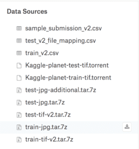
Example of Download Button to Download Files for the Planet Dataset
The specific files required for this tutorial are as follows:
- train-jpg.tar.7z (600MB)
- train_v2.csv.zip (159KB)
Note: the jpeg zip files might be listed without the .7z extension. If so, download the .tar versions.
Once you have downloaded the dataset files, you must unzip them. The .zip files for the CSV files can be unzipped using your favorite unzipping program.
The .7z files that contain the JPEG images can also be unzipped using your favorite unzipping program. If this is a new zip format for you, you may need additional software, such as “The Unarchiver” software on MacOS, or p7zip on many platforms.
For example, on the command line on most POSIX-based workstations the .7z files can be decompressed using the p7zip and tar files as follows:
|
1 2 3 4 |
7z x test-jpg.tar.7z tar -xvf test-jpg.tar 7z x train-jpg.tar.7z tar -xvf train-jpg.tar |
Once unzipped, you will now have a CSV file and a directory in your current working directory, as follows:
|
1 2 |
train-jpg/ train_v2.csv |
Inspecting the folder, you will see many jpeg files.
Inspecting the train_v2.csv file, you will see a mapping of jpeg files in the training dataset (train-jpg/) and their mapping to class labels separated by a space for each; for example:
|
1 2 3 4 5 6 7 |
image_name,tags train_0,haze primary train_1,agriculture clear primary water train_2,clear primary train_3,clear primary train_4,agriculture clear habitation primary road ... |
The dataset must be prepared before modeling.
There are at least two approaches we could explore; they are: an in-memory approach and a progressive loading approach.
The dataset could be prepared with the intent of loading the entire training dataset into memory when fitting models. This will require a machine with sufficient RAM to hold all of the images (e.g. 32GB or 64GB of RAM), such as an Amazon EC2 instance, although training models will be significantly faster.
Alternately, the dataset could be loaded as-needed during training, batch by batch. This would require developing a data generator. Training models would be significantly slower, but training could be performed on workstations with less RAM (e.g. 8GB or 16GB).
In this tutorial, we will use the former approach. As such, I strongly encourage you to run the tutorial on an Amazon EC2 instance with sufficient RAM and access to a GPUs, such as the affordable p3.2xlarge instance on the Deep Learning AMI (Amazon Linux) AMI, which costs approximately $3 USD per hour. For a step-by-step tutorial on how to set up an Amazon EC2 instance for deep learning, see the post:
If using an EC2 instance is not an option for you, then I will give hints below on how to further reduce the size of the training dataset so that it will fit into memory on your workstation so that you can complete this tutorial.
Visualize Dataset
The first step is to inspect some of the images in the training dataset.
We can do this by loading some images and plotting multiple images in one figure using Matplotlib.
The complete example is listed below.
|
1 2 3 4 5 6 7 8 9 10 11 12 13 14 15 16 17 |
# plot the first 9 images in the planet dataset from matplotlib import pyplot from matplotlib.image import imread # define location of dataset folder = 'train-jpg/' # plot first few images for i in range(9): # define subplot pyplot.subplot(330 + 1 + i) # define filename filename = folder + 'train_' + str(i) + '.jpg' # load image pixels image = imread(filename) # plot raw pixel data pyplot.imshow(image) # show the figure pyplot.show() |
Running the example creates a figure that plots the first nine images in the training dataset.
We can see that the images are indeed satellite photos of the rain forest. Some show significant haze, others show show trees, roads, or rivers and other structures.
The plots suggests that modeling may benefit from data augmentation as well as simple techniques to make the features in the images more visible.
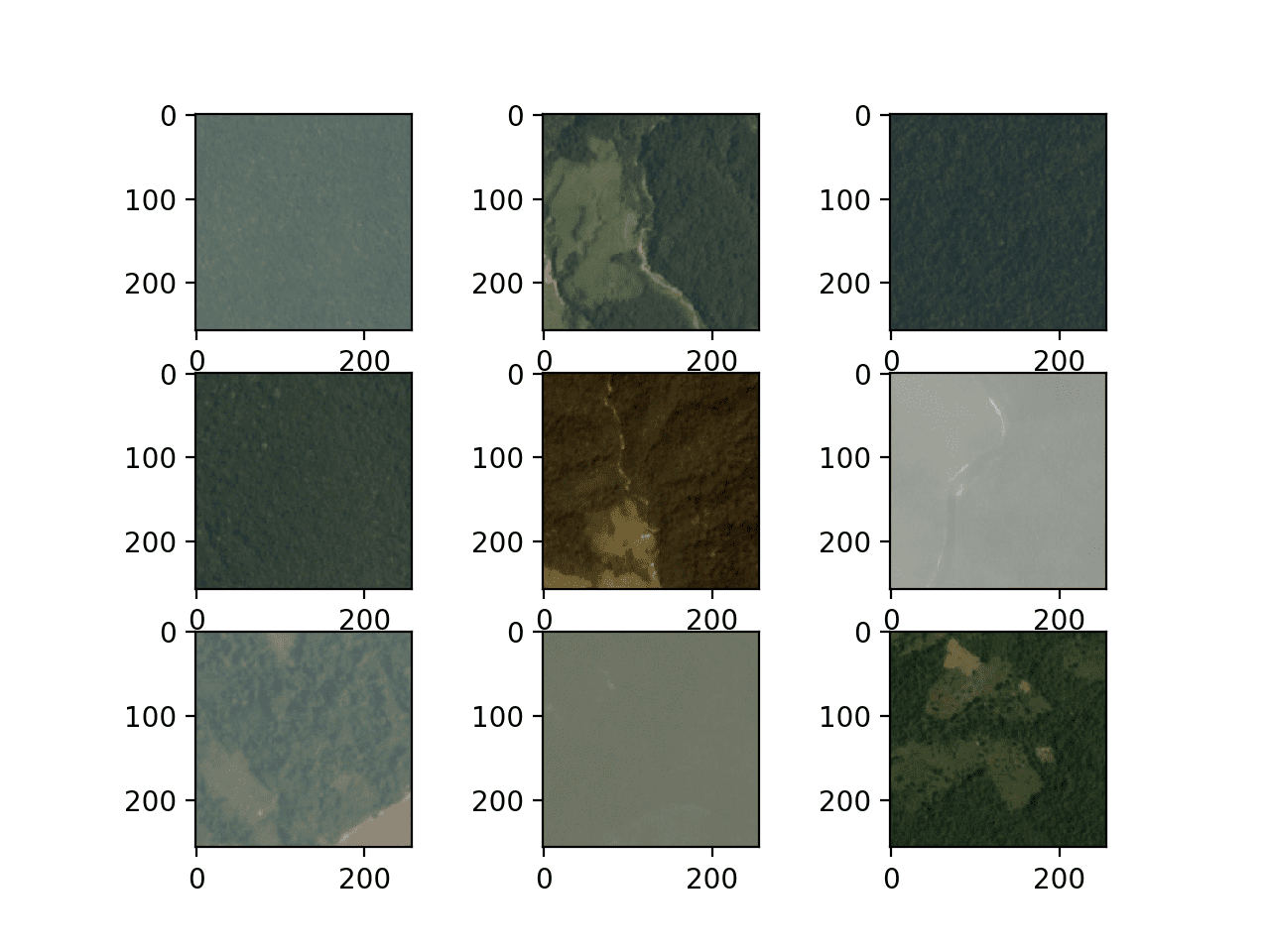
Figure Showing the First Nine Images From the Planet Dataset
Create Mappings
The next step involves understanding the labels that may be assigned to each image.
We can load the CSV mapping file for the training dataset (train_v2.csv) directly using the read_csv() Pandas function.
The complete example is listed below.
|
1 2 3 4 5 6 7 8 |
# load and summarize the mapping file for the planet dataset from pandas import read_csv # load file as CSV filename = 'train_v2.csv' mapping_csv = read_csv(filename) # summarize properties print(mapping_csv.shape) print(mapping_csv[:10]) |
Running the example first summarizes the shape of the training dataset. We can see that there are indeed 40,479 training images known to the mapping file.
Next, the first 10 rows of the file are summarized. We can see that the second column of the file contains a space-separated list of tags to assign to each image.
|
1 2 3 4 5 6 7 8 9 10 11 12 13 |
(40479, 2) image_name tags 0 train_0 haze primary 1 train_1 agriculture clear primary water 2 train_2 clear primary 3 train_3 clear primary 4 train_4 agriculture clear habitation primary road 5 train_5 haze primary water 6 train_6 agriculture clear cultivation primary water 7 train_7 haze primary 8 train_8 agriculture clear cultivation primary 9 train_9 agriculture clear cultivation primary road |
We will need the set of all known tags to be assigned to images, as well as a unique and consistent integer to apply to each tag. This is so that we can develop a target vector for each image with a one hot encoding, e.g. a vector with all zeros and a one at the index for each tag applied to the image.
This can be achieved by looping through each row in the “tags” column, splitting the tags by space, and storing them in a set. We will then have a set of all known tags. For example:
|
1 2 3 4 5 6 7 |
# create a set of labels labels = set() for i in range(len(mapping_csv)): # convert spaced separated tags into an array of tags tags = mapping_csv['tags'][i].split(' ') # add tags to the set of known labels labels.update(tags) |
This can then be ordered alphabetically and each tag assigned an integer based on this alphabetic rank.
This will mean that the same tag will always be assigned the same integer for consistency.
|
1 2 3 4 |
# convert set of labels to a list to list labels = list(labels) # order set alphabetically labels.sort() |
We can create a dictionary that maps tags to integers so that we can encode the training dataset for modeling.
We can also create a dictionary with the reverse mapping from integers to string tag values, so later when the model makes a prediction, we can turn it into something readable.
|
1 2 3 |
# dict that maps labels to integers, and the reverse labels_map = {labels[i]:i for i in range(len(labels))} inv_labels_map = {i:labels[i] for i in range(len(labels))} |
We can tie all of this together into a convenience function called create_tag_mapping() that will take the loaded DataFrame containing the train_v2.csv data and return a mapping and inverse mapping dictionaries.
|
1 2 3 4 5 6 7 8 9 10 11 12 13 14 15 16 17 |
# create a mapping of tags to integers given the loaded mapping file def create_tag_mapping(mapping_csv): # create a set of all known tags labels = set() for i in range(len(mapping_csv)): # convert spaced separated tags into an array of tags tags = mapping_csv['tags'][i].split(' ') # add tags to the set of known labels labels.update(tags) # convert set of labels to a list to list labels = list(labels) # order set alphabetically labels.sort() # dict that maps labels to integers, and the reverse labels_map = {labels[i]:i for i in range(len(labels))} inv_labels_map = {i:labels[i] for i in range(len(labels))} return labels_map, inv_labels_map |
We can test out this function to see how many and what tags we have to work with; the complete example is listed below.
|
1 2 3 4 5 6 7 8 9 10 11 12 13 14 15 16 17 18 19 20 21 22 23 24 25 26 27 28 |
# create a mapping of tags to integers from pandas import read_csv # create a mapping of tags to integers given the loaded mapping file def create_tag_mapping(mapping_csv): # create a set of all known tags labels = set() for i in range(len(mapping_csv)): # convert spaced separated tags into an array of tags tags = mapping_csv['tags'][i].split(' ') # add tags to the set of known labels labels.update(tags) # convert set of labels to a list to list labels = list(labels) # order set alphabetically labels.sort() # dict that maps labels to integers, and the reverse labels_map = {labels[i]:i for i in range(len(labels))} inv_labels_map = {i:labels[i] for i in range(len(labels))} return labels_map, inv_labels_map # load file as CSV filename = 'train_v2.csv' mapping_csv = read_csv(filename) # create a mapping of tags to integers mapping, inv_mapping = create_tag_mapping(mapping_csv) print(len(mapping)) print(mapping) |
Running the example, we can see that we have a total of 17 tags in the dataset.
We can also see the mapping dictionary where each tag is assigned a consistent and unique integer. The tags appear to be sensible descriptions of the types of features we may see in a given satellite image.
It might be interesting as a further extension to explore the distribution of tags across images to see if their assignment or use in the training dataset is balanced or imbalanced. This could give further insight into how difficult the prediction problem may be.
|
1 2 3 |
17 {'agriculture': 0, 'artisinal_mine': 1, 'bare_ground': 2, 'blooming': 3, 'blow_down': 4, 'clear': 5, 'cloudy': 6, 'conventional_mine': 7, 'cultivation': 8, 'habitation': 9, 'haze': 10, 'partly_cloudy': 11, 'primary': 12, 'road': 13, 'selective_logging': 14, 'slash_burn': 15, 'water': 16} |
We also need a mapping of training set filenames to the tags for the image.
This is a simple dictionary with the filename of the image as the key and the list of tags as the value.
The create_file_mapping() below implements this, also taking the loaded DataFrame as an argument and returning the mapping with the tag value for each filename stored as a list.
|
1 2 3 4 5 6 7 |
# create a mapping of filename to tags def create_file_mapping(mapping_csv): mapping = dict() for i in range(len(mapping_csv)): name, tags = mapping_csv['image_name'][i], mapping_csv['tags'][i] mapping[name] = tags.split(' ') return mapping |
We can now prepare the image component of the dataset.
Create In-Memory Dataset
We need to be able to load the JPEG images into memory.
This can be achieved by enumerating all files in the train-jpg/ folder. Keras provides a simple API to load an image from file via the load_img() function and to cover it to a NumPy array via the img_to_array() function.
As part of loading an image, we can force the size to be smaller to save memory and speed up training. In this case, we will halve the size of the image from 256×256 to 128×128. We will also store the pixel values as an unsigned 8-bit integer (e.g. values between 0 and 255).
|
1 2 3 4 |
# load image photo = load_img(filename, target_size=(128,128)) # convert to numpy array photo = img_to_array(photo, dtype='uint8') |
The photo will represent an input to the model, but we require an output for the photo.
We can then retrieve the tags for the loaded image using the filename without the extension using the prepared filename-to-tags mapping prepared with the create_file_mapping() function developed in the previous section.
|
1 2 |
# get tags tags = file_mapping(filename[:-4]) |
We need to one hot encode the tags for the image. This means that we will require a 17-element vector with a 1 value for each tag present. We can get the index of where to place the 1 values from the mapping of tags to integers created via the create_tag_mapping() function developed in the previous section.
The one_hot_encode() function below implements this, given a list of tags for an image and the mapping of tags to integers as arguments, and it will return a 17 element NumPy array that describes a one hot encoding of the tags for one photo.
|
1 2 3 4 5 6 7 8 |
# create a one hot encoding for one list of tags def one_hot_encode(tags, mapping): # create empty vector encoding = zeros(len(mapping), dtype='uint8') # mark 1 for each tag in the vector for tag in tags: encoding[mapping[tag]] = 1 return encoding |
We can now load the input (photos) and output (one hot encoded vector) elements for the entire training dataset.
The load_dataset() function below implements this given the path to the JPEG images, the mapping of files to tags, and the mapping of tags to integers as inputs; it will return NumPy arrays for the X and y elements for modeling.
|
1 2 3 4 5 6 7 8 9 10 11 12 13 14 15 16 17 18 19 |
# load all images into memory def load_dataset(path, file_mapping, tag_mapping): photos, targets = list(), list() # enumerate files in the directory for filename in listdir(folder): # load image photo = load_img(path + filename, target_size=(128,128)) # convert to numpy array photo = img_to_array(photo, dtype='uint8') # get tags tags = file_mapping[filename[:-4]] # one hot encode tags target = one_hot_encode(tags, tag_mapping) # store photos.append(photo) targets.append(target) X = asarray(photos, dtype='uint8') y = asarray(targets, dtype='uint8') return X, y |
Note: this will load the entire training dataset into memory and may require at least 128x128x3 x 40,479 images x 8 bits, or about 2 GB RAM just to hold the loaded photos.
If you run out of memory here, or later when modeling (when pixels are 16 or 32 bits), try reducing the size of the loaded photos to 32×32 and/or stop the loop after loading 20,000 photographs.
Once loaded, we can save these NumPy arrays to file for later use.
We could use the save() or savez() NumPy functions to save the arrays direction. Instead, we will use the savez_compressed() NumPy function to save both arrays in one function call in a compressed format, saving a few more megabytes. Loading the arrays of smaller images will be significantly faster than loading the raw JPEG images each time during modeling.
|
1 2 |
# save both arrays to one file in compressed format savez_compressed('planet_data.npz', X, y) |
We can tie all of this together and prepare the Planet dataset for in-memory modeling and save it to a new single file for fast loading later.
The complete example is listed below.
|
1 2 3 4 5 6 7 8 9 10 11 12 13 14 15 16 17 18 19 20 21 22 23 24 25 26 27 28 29 30 31 32 33 34 35 36 37 38 39 40 41 42 43 44 45 46 47 48 49 50 51 52 53 54 55 56 57 58 59 60 61 62 63 64 65 66 67 68 69 70 71 72 73 74 75 76 77 |
# load and prepare planet dataset and save to file from os import listdir from numpy import zeros from numpy import asarray from numpy import savez_compressed from pandas import read_csv from keras.preprocessing.image import load_img from keras.preprocessing.image import img_to_array # create a mapping of tags to integers given the loaded mapping file def create_tag_mapping(mapping_csv): # create a set of all known tags labels = set() for i in range(len(mapping_csv)): # convert spaced separated tags into an array of tags tags = mapping_csv['tags'][i].split(' ') # add tags to the set of known labels labels.update(tags) # convert set of labels to a list to list labels = list(labels) # order set alphabetically labels.sort() # dict that maps labels to integers, and the reverse labels_map = {labels[i]:i for i in range(len(labels))} inv_labels_map = {i:labels[i] for i in range(len(labels))} return labels_map, inv_labels_map # create a mapping of filename to a list of tags def create_file_mapping(mapping_csv): mapping = dict() for i in range(len(mapping_csv)): name, tags = mapping_csv['image_name'][i], mapping_csv['tags'][i] mapping[name] = tags.split(' ') return mapping # create a one hot encoding for one list of tags def one_hot_encode(tags, mapping): # create empty vector encoding = zeros(len(mapping), dtype='uint8') # mark 1 for each tag in the vector for tag in tags: encoding[mapping[tag]] = 1 return encoding # load all images into memory def load_dataset(path, file_mapping, tag_mapping): photos, targets = list(), list() # enumerate files in the directory for filename in listdir(folder): # load image photo = load_img(path + filename, target_size=(128,128)) # convert to numpy array photo = img_to_array(photo, dtype='uint8') # get tags tags = file_mapping[filename[:-4]] # one hot encode tags target = one_hot_encode(tags, tag_mapping) # store photos.append(photo) targets.append(target) X = asarray(photos, dtype='uint8') y = asarray(targets, dtype='uint8') return X, y # load the mapping file filename = 'train_v2.csv' mapping_csv = read_csv(filename) # create a mapping of tags to integers tag_mapping, _ = create_tag_mapping(mapping_csv) # create a mapping of filenames to tag lists file_mapping = create_file_mapping(mapping_csv) # load the jpeg images folder = 'train-jpg/' X, y = load_dataset(folder, file_mapping, tag_mapping) print(X.shape, y.shape) # save both arrays to one file in compressed format savez_compressed('planet_data.npz', X, y) |
Running the example first loads the entire dataset and summarizes the shape. We can confirm that the input samples (X) are 128×128 color images and that the output samples are 17-element vectors.
At the end of the run, a single file ‘planet_data.npz‘ is saved containing the dataset that is approximately 1.2 gigabytes in size, saving about 700 megabytes due to compression.
|
1 |
(40479, 128, 128, 3) (40479, 17) |
The dataset can be loaded easily later using the load() NumPy function, as follows:
|
1 2 3 4 5 |
# load prepared planet dataset from numpy import load data = load('planet_data.npz') X, y = data['arr_0'], data['arr_1'] print('Loaded: ', X.shape, y.shape) |
Running this small example confirms that the dataset is correctly loaded.
|
1 |
Loaded: (40479, 128, 128, 3) (40479, 17) |
Model Evaluation Measure
Before we start modeling, we must select a performance metric.
Classification accuracy is often appropriate for binary classification tasks with a balanced number of examples in each class.
In this case, we are working neither with a binary or multi-class classification task; instead, it is a multi-label classification task and the number of labels are not balanced, with some used more heavily than others.
As such, the Kaggle competition organizes chose the F-beta metric, specifically the F2 score. This is a metric that is related to the F1 score (also called F-measure).
The F1 score calculates the average of the recall and the precision. You may remember that the precision and recall are calculated as follows:
|
1 2 |
precision = true positives / (true positives + false positives) recall = true positives / (true positives + false negatives) |
Precision describes how good a model is at predicting the positive class. Recall describes how good the model is at predicting the positive class when the actual outcome is positive.
The F1 is the mean of these two scores, specifically the harmonic mean instead of the arithmetic mean because the values are proportions. F1 is preferred over accuracy when evaluating the performance of a model on an imbalanced dataset, with a value between 0 and 1 for worst and best possible scores.
|
1 |
F1 = 2 x (precision x recall) / (precision + recall) |
The F-beta metric is a generalization of F1 that allows a term called beta to be introduced that weights how important recall is compared to precision when calculating the mean
|
1 |
F-Beta = (1 + Beta^2) x (precision x recall) / (Beta^2 x precision + recall) |
A common value of beta is two, and this was the value used in the competition, where recall valued twice as highly as precision. This is often referred to as the F2 score.
The idea of a positive and negative class only makes sense for a binary classification problem. As we are predicting multiple classes, the idea of positive and negative and related terms are calculated for each class in a one vs. rest manner, then averaged across each class.
The scikit-learn library provides an implementation of F-beta via the fbeta_score() function. We can call this function to evaluate a set of predictions and specify a beta value of 2 and the “average” argument set to “samples“.
|
1 |
score = fbeta_score(y_true, y_pred, 2, average='samples') |
For example, we can test this on our prepared dataset.
We can split our loaded dataset into separate train and test datasets that we can use to train and evaluate models on this problem. This can be achieved using the train_test_split() and specifying a ‘random_state‘ argument so that the same data split is given each time the code is run.
We will use 70% for the training set and 30% for the test set.
|
1 |
trainX, testX, trainY, testY = train_test_split(X, y, test_size=0.3, random_state=1) |
The load_dataset() function below implements this by loading the saved dataset, splitting it into train and test components, and returning them ready for use.
|
1 2 3 4 5 6 7 8 9 |
# load train and test dataset def load_dataset(): # load dataset data = load('planet_data.npz') X, y = data['arr_0'], data['arr_1'] # separate into train and test datasets trainX, testX, trainY, testY = train_test_split(X, y, test_size=0.3, random_state=1) print(trainX.shape, trainY.shape, testX.shape, testY.shape) return trainX, trainY, testX, testY |
We can then make a prediction of all classes or all 1 values in the one hot encoded vectors.
|
1 2 3 |
# make all one predictions train_yhat = asarray([ones(trainY.shape[1]) for _ in range(trainY.shape[0])]) test_yhat = asarray([ones(testY.shape[1]) for _ in range(testY.shape[0])]) |
The predictions can then be evaluated using the scikit-learn fbeta_score() function with the true values in the train and test dataset.
|
1 2 |
train_score = fbeta_score(trainY, train_yhat, 2, average='samples') test_score = fbeta_score(testY, test_yhat, 2, average='samples') |
Tying this together, the complete example is listed below.
|
1 2 3 4 5 6 7 8 9 10 11 12 13 14 15 16 17 18 19 20 21 22 23 24 25 26 |
# test f-beta score from numpy import load from numpy import ones from numpy import asarray from sklearn.model_selection import train_test_split from sklearn.metrics import fbeta_score # load train and test dataset def load_dataset(): # load dataset data = load('planet_data.npz') X, y = data['arr_0'], data['arr_1'] # separate into train and test datasets trainX, testX, trainY, testY = train_test_split(X, y, test_size=0.3, random_state=1) print(trainX.shape, trainY.shape, testX.shape, testY.shape) return trainX, trainY, testX, testY # load dataset trainX, trainY, testX, testY = load_dataset() # make all one predictions train_yhat = asarray([ones(trainY.shape[1]) for _ in range(trainY.shape[0])]) test_yhat = asarray([ones(testY.shape[1]) for _ in range(testY.shape[0])]) # evaluate predictions train_score = fbeta_score(trainY, train_yhat, 2, average='samples') test_score = fbeta_score(testY, test_yhat, 2, average='samples') print('All Ones: train=%.3f, test=%.3f' % (train_score, test_score)) |
Running this example first loads the prepared dataset, then splits it into train and test sets and the shape of the prepared datasets is reported. We can see that we have a little more than 28,000 examples in the training dataset and a little more than 12,000 examples in the test set.
Next, the all-one predictions are prepared and then evaluated and the scores are reported. We can see that an all ones prediction for both datasets results in a score of about 0.48.
|
1 2 |
(28335, 128, 128, 3) (28335, 17) (12144, 128, 128, 3) (12144, 17) All Ones: train=0.484, test=0.483 |
We will require a version of the F-beta score calculation in Keras to use as a metric.
Keras used to support this metric for binary classification problems (2 classes) prior to version 2.0 of the library; we can see the code for this older version here: metrics.py. This code can be used as the basis for defining a new metric function that can be used with Keras. A version of this function is also proposed in a Kaggle kernel titled “F-beta score for Keras“. This new function is listed below.
|
1 2 3 4 5 6 7 8 9 10 11 12 13 14 15 16 17 18 |
from keras import backend # calculate fbeta score for multi-class/label classification def fbeta(y_true, y_pred, beta=2): # clip predictions y_pred = backend.clip(y_pred, 0, 1) # calculate elements tp = backend.sum(backend.round(backend.clip(y_true * y_pred, 0, 1)), axis=1) fp = backend.sum(backend.round(backend.clip(y_pred - y_true, 0, 1)), axis=1) fn = backend.sum(backend.round(backend.clip(y_true - y_pred, 0, 1)), axis=1) # calculate precision p = tp / (tp + fp + backend.epsilon()) # calculate recall r = tp / (tp + fn + backend.epsilon()) # calculate fbeta, averaged across each class bb = beta ** 2 fbeta_score = backend.mean((1 + bb) * (p * r) / (bb * p + r + backend.epsilon())) return fbeta_score |
It can be used when compiling a model in Keras, specified via the metrics argument; for example:
|
1 2 |
... model.compile(... metrics=[fbeta]) |
We can test this new function and compare results to the scikit-learn function as follows.
|
1 2 3 4 5 6 7 8 9 10 11 12 13 14 15 16 17 18 19 20 21 22 23 24 25 26 27 28 29 30 31 32 33 34 35 36 37 38 39 40 41 42 43 44 45 46 47 48 |
# compare f-beta score between sklearn and keras from numpy import load from numpy import ones from numpy import asarray from sklearn.model_selection import train_test_split from sklearn.metrics import fbeta_score from keras import backend # load train and test dataset def load_dataset(): # load dataset data = load('planet_data.npz') X, y = data['arr_0'], data['arr_1'] # separate into train and test datasets trainX, testX, trainY, testY = train_test_split(X, y, test_size=0.3, random_state=1) print(trainX.shape, trainY.shape, testX.shape, testY.shape) return trainX, trainY, testX, testY # calculate fbeta score for multi-class/label classification def fbeta(y_true, y_pred, beta=2): # clip predictions y_pred = backend.clip(y_pred, 0, 1) # calculate elements tp = backend.sum(backend.round(backend.clip(y_true * y_pred, 0, 1)), axis=1) fp = backend.sum(backend.round(backend.clip(y_pred - y_true, 0, 1)), axis=1) fn = backend.sum(backend.round(backend.clip(y_true - y_pred, 0, 1)), axis=1) # calculate precision p = tp / (tp + fp + backend.epsilon()) # calculate recall r = tp / (tp + fn + backend.epsilon()) # calculate fbeta, averaged across each class bb = beta ** 2 fbeta_score = backend.mean((1 + bb) * (p * r) / (bb * p + r + backend.epsilon())) return fbeta_score # load dataset trainX, trainY, testX, testY = load_dataset() # make all one predictions train_yhat = asarray([ones(trainY.shape[1]) for _ in range(trainY.shape[0])]) test_yhat = asarray([ones(testY.shape[1]) for _ in range(testY.shape[0])]) # evaluate predictions with sklearn train_score = fbeta_score(trainY, train_yhat, 2, average='samples') test_score = fbeta_score(testY, test_yhat, 2, average='samples') print('All Ones (sklearn): train=%.3f, test=%.3f' % (train_score, test_score)) # evaluate predictions with keras train_score = fbeta(backend.variable(trainY), backend.variable(train_yhat)) test_score = fbeta(backend.variable(testY), backend.variable(test_yhat)) print('All Ones (keras): train=%.3f, test=%.3f' % (train_score, test_score)) |
Running the example loads the datasets as before, and in this case, the F-beta is calculated using both scikit-learn and Keras. We can see that both functions achieve the same result.
|
1 2 3 |
(28335, 128, 128, 3) (28335, 17) (12144, 128, 128, 3) (12144, 17) All Ones (sklearn): train=0.484, test=0.483 All Ones (keras): train=0.484, test=0.483 |
We can use the score of 0.483 on the test set as a naive forecast to which all models in the subsequent sections can be compared to determine if they are skillful or not.
How to Evaluate a Baseline Model
We are now ready to develop and evaluate a baseline convolutional neural network model for the prepared planet dataset.
We will design a baseline model with a VGG-type structure. That is blocks of convolutional layers with small 3×3 filters followed by a max pooling layer, with this pattern repeating with a doubling in the number of filters with each block added.
Specifically, each block will have two convolutional layers with 3×3 filters, ReLU activation and He weight initialization with same padding, ensuring the output feature maps have the same width and height. These will be followed by a max pooling layer with a 3×3 kernel. Three of these blocks will be used with 32, 64 and 128 filters respectively.
|
1 2 3 4 5 6 7 8 9 10 |
model = Sequential() model.add(Conv2D(32, (3, 3), activation='relu', kernel_initializer='he_uniform', padding='same', input_shape=(128, 128, 3))) model.add(Conv2D(32, (3, 3), activation='relu', kernel_initializer='he_uniform', padding='same')) model.add(MaxPooling2D((2, 2))) model.add(Conv2D(64, (3, 3), activation='relu', kernel_initializer='he_uniform', padding='same')) model.add(Conv2D(64, (3, 3), activation='relu', kernel_initializer='he_uniform', padding='same')) model.add(MaxPooling2D((2, 2))) model.add(Conv2D(128, (3, 3), activation='relu', kernel_initializer='he_uniform', padding='same')) model.add(Conv2D(128, (3, 3), activation='relu', kernel_initializer='he_uniform', padding='same')) model.add(MaxPooling2D((2, 2))) |
The output of the final pooling layer will be flattened and fed to a fully connected layer for interpretation then finally to an output layer for prediction.
The model must produce a 17-element vector with a prediction between 0 and 1 for each output class.
|
1 2 3 |
model.add(Flatten()) model.add(Dense(128, activation='relu', kernel_initializer='he_uniform')) model.add(Dense(17, activation='sigmoid')) |
If this were a multi-class classification problem, we would use a softmax activation function and the categorical cross entropy loss function. This would not be appropriate for multi-label classification, as we expect the model to output multiple 1 values, not a single 1 value. In this case, we will use the sigmoid activation function in the output layer and optimize the binary cross entropy loss function.
The model will be optimized with mini-batch stochastic gradient descent with a conservative learning rate of 0.01 and a momentum of 0.9, and the model will keep track of the “fbeta” metric during training.
|
1 2 3 |
# compile model opt = SGD(lr=0.01, momentum=0.9) model.compile(optimizer=opt, loss='binary_crossentropy', metrics=[fbeta]) |
The define_model() function below ties all of this together and parameterized the shape of the input and output, in case you want to experiment by changing these values or reuse the code on another dataset.
The function will return a model ready to be fit on the planet dataset.
|
1 2 3 4 5 6 7 8 9 10 11 12 13 14 15 16 17 18 19 |
# define cnn model def define_model(in_shape=(128, 128, 3), out_shape=17): model = Sequential() model.add(Conv2D(32, (3, 3), activation='relu', kernel_initializer='he_uniform', padding='same', input_shape=in_shape)) model.add(Conv2D(32, (3, 3), activation='relu', kernel_initializer='he_uniform', padding='same')) model.add(MaxPooling2D((2, 2))) model.add(Conv2D(64, (3, 3), activation='relu', kernel_initializer='he_uniform', padding='same')) model.add(Conv2D(64, (3, 3), activation='relu', kernel_initializer='he_uniform', padding='same')) model.add(MaxPooling2D((2, 2))) model.add(Conv2D(128, (3, 3), activation='relu', kernel_initializer='he_uniform', padding='same')) model.add(Conv2D(128, (3, 3), activation='relu', kernel_initializer='he_uniform', padding='same')) model.add(MaxPooling2D((2, 2))) model.add(Flatten()) model.add(Dense(128, activation='relu', kernel_initializer='he_uniform')) model.add(Dense(out_shape, activation='sigmoid')) # compile model opt = SGD(lr=0.01, momentum=0.9) model.compile(optimizer=opt, loss='binary_crossentropy', metrics=[fbeta]) return model |
The choice of this model as the baseline model is somewhat arbitrary. You may want to explore with other baseline models that have fewer layers or different learning rates.
We can use the load_dataset() function developed in the previous section to load the dataset and split it into train and test sets for fitting and evaluating a defined model.
The pixel values will be normalized before fitting the model. We will achieve this by defining an ImageDataGenerator instance and specify the rescale argument as 1.0/255.0. This will normalize pixel values per batch to 32-bit floating point values, which might be more memory efficient than rescaling all of the pixel values at once in memory.
|
1 2 |
# create data generator datagen = ImageDataGenerator(rescale=1.0/255.0) |
We can create iterators from this data generator for both the train and test sets, and in this case, we will use the relatively large batch size of 128 images to accelerate learning.
|
1 2 3 |
# prepare iterators train_it = datagen.flow(trainX, trainY, batch_size=128) test_it = datagen.flow(testX, testY, batch_size=128) |
The defined model can then be fit using the train iterator, and the test iterator can be used to evaluate the test dataset at the end of each epoch. The model will be fit for 50 epochs.
|
1 2 3 |
# fit model history = model.fit_generator(train_it, steps_per_epoch=len(train_it), validation_data=test_it, validation_steps=len(test_it), epochs=50, verbose=0) |
Once fit, we can calculate the final loss and F-beta scores on the test dataset to estimate the skill of the model.
|
1 2 3 |
# evaluate model loss, fbeta = model.evaluate_generator(test_it, steps=len(test_it), verbose=0) print('> loss=%.3f, fbeta=%.3f' % (loss, fbeta)) |
The fit_generator() function called to fit the model returns a dictionary containing the loss and F-beta scores recorded each epoch on the train and test dataset. We can create a plot of these traces that can provide insight into the learning dynamics of the model.
The summarize_diagnostics() function will create a figure from this recorded history data with one plot showing loss and another the F-beta scores for the model at the end of each training epoch on the train dataset (blue lines) and test dataset (orange lines).
The created figure is saved to a PNG file with the same filename as the script with a “_plot.png” extension. This allows the same test harness to be used with multiple different script files for different model configurations, saving the learning curves in separate files along the way.
|
1 2 3 4 5 6 7 8 9 10 11 12 13 14 15 16 |
# plot diagnostic learning curves def summarize_diagnostics(history): # plot loss pyplot.subplot(211) pyplot.title('Cross Entropy Loss') pyplot.plot(history.history['loss'], color='blue', label='train') pyplot.plot(history.history['val_loss'], color='orange', label='test') # plot accuracy pyplot.subplot(212) pyplot.title('Fbeta') pyplot.plot(history.history['fbeta'], color='blue', label='train') pyplot.plot(history.history['val_fbeta'], color='orange', label='test') # save plot to file filename = sys.argv[0].split('/')[-1] pyplot.savefig(filename + '_plot.png') pyplot.close() |
We can tie this together and define a function run_test_harness() to drive the test harness, including the loading and preparation of the data as well as definition, fit, and evaluation of the model.
|
1 2 3 4 5 6 7 8 9 10 11 12 13 14 15 16 17 18 19 |
# run the test harness for evaluating a model def run_test_harness(): # load dataset trainX, trainY, testX, testY = load_dataset() # create data generator datagen = ImageDataGenerator(rescale=1.0/255.0) # prepare iterators train_it = datagen.flow(trainX, trainY, batch_size=128) test_it = datagen.flow(testX, testY, batch_size=128) # define model model = define_model() # fit model history = model.fit_generator(train_it, steps_per_epoch=len(train_it), validation_data=test_it, validation_steps=len(test_it), epochs=50, verbose=0) # evaluate model loss, fbeta = model.evaluate_generator(test_it, steps=len(test_it), verbose=0) print('> loss=%.3f, fbeta=%.3f' % (loss, fbeta)) # learning curves summarize_diagnostics(history) |
The complete example of evaluating a baseline model on the planet dataset is listed below.
|
1 2 3 4 5 6 7 8 9 10 11 12 13 14 15 16 17 18 19 20 21 22 23 24 25 26 27 28 29 30 31 32 33 34 35 36 37 38 39 40 41 42 43 44 45 46 47 48 49 50 51 52 53 54 55 56 57 58 59 60 61 62 63 64 65 66 67 68 69 70 71 72 73 74 75 76 77 78 79 80 81 82 83 84 85 86 87 88 89 90 91 92 93 94 95 96 97 98 99 100 |
# baseline model for the planet dataset import sys from numpy import load from matplotlib import pyplot from sklearn.model_selection import train_test_split from keras import backend from keras.preprocessing.image import ImageDataGenerator from keras.models import Sequential from keras.layers import Conv2D from keras.layers import MaxPooling2D from keras.layers import Dense from keras.layers import Flatten from keras.optimizers import SGD # load train and test dataset def load_dataset(): # load dataset data = load('planet_data.npz') X, y = data['arr_0'], data['arr_1'] # separate into train and test datasets trainX, testX, trainY, testY = train_test_split(X, y, test_size=0.3, random_state=1) print(trainX.shape, trainY.shape, testX.shape, testY.shape) return trainX, trainY, testX, testY # calculate fbeta score for multi-class/label classification def fbeta(y_true, y_pred, beta=2): # clip predictions y_pred = backend.clip(y_pred, 0, 1) # calculate elements tp = backend.sum(backend.round(backend.clip(y_true * y_pred, 0, 1)), axis=1) fp = backend.sum(backend.round(backend.clip(y_pred - y_true, 0, 1)), axis=1) fn = backend.sum(backend.round(backend.clip(y_true - y_pred, 0, 1)), axis=1) # calculate precision p = tp / (tp + fp + backend.epsilon()) # calculate recall r = tp / (tp + fn + backend.epsilon()) # calculate fbeta, averaged across each class bb = beta ** 2 fbeta_score = backend.mean((1 + bb) * (p * r) / (bb * p + r + backend.epsilon())) return fbeta_score # define cnn model def define_model(in_shape=(128, 128, 3), out_shape=17): model = Sequential() model.add(Conv2D(32, (3, 3), activation='relu', kernel_initializer='he_uniform', padding='same', input_shape=in_shape)) model.add(Conv2D(32, (3, 3), activation='relu', kernel_initializer='he_uniform', padding='same')) model.add(MaxPooling2D((2, 2))) model.add(Conv2D(64, (3, 3), activation='relu', kernel_initializer='he_uniform', padding='same')) model.add(Conv2D(64, (3, 3), activation='relu', kernel_initializer='he_uniform', padding='same')) model.add(MaxPooling2D((2, 2))) model.add(Conv2D(128, (3, 3), activation='relu', kernel_initializer='he_uniform', padding='same')) model.add(Conv2D(128, (3, 3), activation='relu', kernel_initializer='he_uniform', padding='same')) model.add(MaxPooling2D((2, 2))) model.add(Flatten()) model.add(Dense(128, activation='relu', kernel_initializer='he_uniform')) model.add(Dense(out_shape, activation='sigmoid')) # compile model opt = SGD(lr=0.01, momentum=0.9) model.compile(optimizer=opt, loss='binary_crossentropy', metrics=[fbeta]) return model # plot diagnostic learning curves def summarize_diagnostics(history): # plot loss pyplot.subplot(211) pyplot.title('Cross Entropy Loss') pyplot.plot(history.history['loss'], color='blue', label='train') pyplot.plot(history.history['val_loss'], color='orange', label='test') # plot accuracy pyplot.subplot(212) pyplot.title('Fbeta') pyplot.plot(history.history['fbeta'], color='blue', label='train') pyplot.plot(history.history['val_fbeta'], color='orange', label='test') # save plot to file filename = sys.argv[0].split('/')[-1] pyplot.savefig(filename + '_plot.png') pyplot.close() # run the test harness for evaluating a model def run_test_harness(): # load dataset trainX, trainY, testX, testY = load_dataset() # create data generator datagen = ImageDataGenerator(rescale=1.0/255.0) # prepare iterators train_it = datagen.flow(trainX, trainY, batch_size=128) test_it = datagen.flow(testX, testY, batch_size=128) # define model model = define_model() # fit model history = model.fit_generator(train_it, steps_per_epoch=len(train_it), validation_data=test_it, validation_steps=len(test_it), epochs=50, verbose=0) # evaluate model loss, fbeta = model.evaluate_generator(test_it, steps=len(test_it), verbose=0) print('> loss=%.3f, fbeta=%.3f' % (loss, fbeta)) # learning curves summarize_diagnostics(history) # entry point, run the test harness run_test_harness() |
Running the example first loads the dataset and splits it into train and test sets. The shape of the input and output elements of each of the train and test datasets is printed, confirming that the same data split was performed as before.
The model is fit and evaluated, and an F-beta score for the final model on the test dataset is reported.
Note: Your results may vary given the stochastic nature of the algorithm or evaluation procedure, or differences in numerical precision. Consider running the example a few times and compare the average outcome.
In this case, the baseline model achieved an F-beta score of about 0.831, which is quite a bit better than the naive score of 0.483 reported in the previous section. This suggests that the baseline model is skillful.
|
1 2 |
(28335, 128, 128, 3) (28335, 17) (12144, 128, 128, 3) (12144, 17) > loss=0.470, fbeta=0.831 |
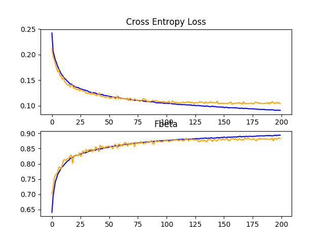
A figure is also created and saved to file showing plots of the learning curves for the model on the train and test sets with regard to both loss and F-beta.
In this case, the plot of the loss learning curves suggests that the model has overfit the training dataset, perhaps around epoch 20 out of 50, although the overfitting has not seemingly negatively impacted the performance of the model on the test dataset with regard to the F-beta score.
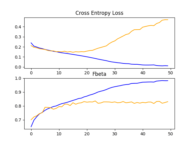
Line Plots Showing Loss and F-Beta Learning Curves for the Baseline Model on the Train and Test Datasets on the Planet Problem
Now that we have a baseline model for the dataset, we have a strong basis for experimentation and improvement.
We will explore some ideas for improving the performance of the model in the next section.
How to Improve Model Performance
In the previous section, we defined a baseline model that can be used as the basis for improvement on the planet dataset.
The model achieved a reasonable F-beta score, although the learning curves suggested that the model had overfit the training dataset. Two common approaches to explore to address overfitting are dropout regularization and data augmentation. Both have the effect of disrupting and slowing down the learning process, specifically the rate that the model improves over training epochs.
We will explore both of these methods in this section. Given that we expect the rate of learning to be slowed, we give the model more time to learn by increasing the number of training epochs from 50 to 200.
Dropout Regularization
Dropout regularization is a computationally cheap way to regularize a deep neural network.
Dropout works by probabilistically removing, or “dropping out,” inputs to a layer, which may be input variables in the data sample or activations from a previous layer. It has the effect of simulating a large number of networks with very different network structure and, in turn, making nodes in the network generally more robust to the inputs.
For more information on dropout, see the post:
Typically, a small amount of dropout can be applied after each VGG block, with more dropout applied to the fully connected layers near the output layer of the model.
Below is the define_model() function for an updated version of the baseline model with the addition of Dropout. In this case, a dropout of 20% is applied after each VGG block, with a larger dropout rate of 50% applied after the fully connected layer in the classifier part of the model.
|
1 2 3 4 5 6 7 8 9 10 11 12 13 14 15 16 17 18 19 20 21 22 23 |
# define cnn model def define_model(in_shape=(128, 128, 3), out_shape=17): model = Sequential() model.add(Conv2D(32, (3, 3), activation='relu', kernel_initializer='he_uniform', padding='same', input_shape=in_shape)) model.add(Conv2D(32, (3, 3), activation='relu', kernel_initializer='he_uniform', padding='same')) model.add(MaxPooling2D((2, 2))) model.add(Dropout(0.2)) model.add(Conv2D(64, (3, 3), activation='relu', kernel_initializer='he_uniform', padding='same')) model.add(Conv2D(64, (3, 3), activation='relu', kernel_initializer='he_uniform', padding='same')) model.add(MaxPooling2D((2, 2))) model.add(Dropout(0.2)) model.add(Conv2D(128, (3, 3), activation='relu', kernel_initializer='he_uniform', padding='same')) model.add(Conv2D(128, (3, 3), activation='relu', kernel_initializer='he_uniform', padding='same')) model.add(MaxPooling2D((2, 2))) model.add(Dropout(0.2)) model.add(Flatten()) model.add(Dense(128, activation='relu', kernel_initializer='he_uniform')) model.add(Dropout(0.5)) model.add(Dense(out_shape, activation='sigmoid')) # compile model opt = SGD(lr=0.01, momentum=0.9) model.compile(optimizer=opt, loss='binary_crossentropy', metrics=[fbeta]) return model |
The full code listing of the baseline model with the addition of dropout on the planet dataset is listed below for completeness.
|
1 2 3 4 5 6 7 8 9 10 11 12 13 14 15 16 17 18 19 20 21 22 23 24 25 26 27 28 29 30 31 32 33 34 35 36 37 38 39 40 41 42 43 44 45 46 47 48 49 50 51 52 53 54 55 56 57 58 59 60 61 62 63 64 65 66 67 68 69 70 71 72 73 74 75 76 77 78 79 80 81 82 83 84 85 86 87 88 89 90 91 92 93 94 95 96 97 98 99 100 101 102 103 104 105 |
# baseline model with dropout on the planet dataset import sys from numpy import load from matplotlib import pyplot from sklearn.model_selection import train_test_split from keras import backend from keras.preprocessing.image import ImageDataGenerator from keras.models import Sequential from keras.layers import Conv2D from keras.layers import MaxPooling2D from keras.layers import Dense from keras.layers import Flatten from keras.layers import Dropout from keras.optimizers import SGD # load train and test dataset def load_dataset(): # load dataset data = load('planet_data.npz') X, y = data['arr_0'], data['arr_1'] # separate into train and test datasets trainX, testX, trainY, testY = train_test_split(X, y, test_size=0.3, random_state=1) print(trainX.shape, trainY.shape, testX.shape, testY.shape) return trainX, trainY, testX, testY # calculate fbeta score for multi-class/label classification def fbeta(y_true, y_pred, beta=2): # clip predictions y_pred = backend.clip(y_pred, 0, 1) # calculate elements tp = backend.sum(backend.round(backend.clip(y_true * y_pred, 0, 1)), axis=1) fp = backend.sum(backend.round(backend.clip(y_pred - y_true, 0, 1)), axis=1) fn = backend.sum(backend.round(backend.clip(y_true - y_pred, 0, 1)), axis=1) # calculate precision p = tp / (tp + fp + backend.epsilon()) # calculate recall r = tp / (tp + fn + backend.epsilon()) # calculate fbeta, averaged across each class bb = beta ** 2 fbeta_score = backend.mean((1 + bb) * (p * r) / (bb * p + r + backend.epsilon())) return fbeta_score # define cnn model def define_model(in_shape=(128, 128, 3), out_shape=17): model = Sequential() model.add(Conv2D(32, (3, 3), activation='relu', kernel_initializer='he_uniform', padding='same', input_shape=in_shape)) model.add(Conv2D(32, (3, 3), activation='relu', kernel_initializer='he_uniform', padding='same')) model.add(MaxPooling2D((2, 2))) model.add(Dropout(0.2)) model.add(Conv2D(64, (3, 3), activation='relu', kernel_initializer='he_uniform', padding='same')) model.add(Conv2D(64, (3, 3), activation='relu', kernel_initializer='he_uniform', padding='same')) model.add(MaxPooling2D((2, 2))) model.add(Dropout(0.2)) model.add(Conv2D(128, (3, 3), activation='relu', kernel_initializer='he_uniform', padding='same')) model.add(Conv2D(128, (3, 3), activation='relu', kernel_initializer='he_uniform', padding='same')) model.add(MaxPooling2D((2, 2))) model.add(Dropout(0.2)) model.add(Flatten()) model.add(Dense(128, activation='relu', kernel_initializer='he_uniform')) model.add(Dropout(0.5)) model.add(Dense(out_shape, activation='sigmoid')) # compile model opt = SGD(lr=0.01, momentum=0.9) model.compile(optimizer=opt, loss='binary_crossentropy', metrics=[fbeta]) return model # plot diagnostic learning curves def summarize_diagnostics(history): # plot loss pyplot.subplot(211) pyplot.title('Cross Entropy Loss') pyplot.plot(history.history['loss'], color='blue', label='train') pyplot.plot(history.history['val_loss'], color='orange', label='test') # plot accuracy pyplot.subplot(212) pyplot.title('Fbeta') pyplot.plot(history.history['fbeta'], color='blue', label='train') pyplot.plot(history.history['val_fbeta'], color='orange', label='test') # save plot to file filename = sys.argv[0].split('/')[-1] pyplot.savefig(filename + '_plot.png') pyplot.close() # run the test harness for evaluating a model def run_test_harness(): # load dataset trainX, trainY, testX, testY = load_dataset() # create data generator datagen = ImageDataGenerator(rescale=1.0/255.0) # prepare iterators train_it = datagen.flow(trainX, trainY, batch_size=128) test_it = datagen.flow(testX, testY, batch_size=128) # define model model = define_model() # fit model history = model.fit_generator(train_it, steps_per_epoch=len(train_it), validation_data=test_it, validation_steps=len(test_it), epochs=200, verbose=0) # evaluate model loss, fbeta = model.evaluate_generator(test_it, steps=len(test_it), verbose=0) print('> loss=%.3f, fbeta=%.3f' % (loss, fbeta)) # learning curves summarize_diagnostics(history) # entry point, run the test harness run_test_harness() |
Running the example first fits the model, then reports the model performance on the hold out test dataset.
Note: Your results may vary given the stochastic nature of the algorithm or evaluation procedure, or differences in numerical precision. Consider running the example a few times and compare the average outcome.
In this case, we can see a small lift in model performance from an F-beta score of about 0.831 for the baseline model to about 0.859 with the addition of dropout.
|
1 2 |
(28335, 128, 128, 3) (28335, 17) (12144, 128, 128, 3) (12144, 17) > loss=0.190, fbeta=0.859 |
Reviewing the learning curves, we can see that dropout has had some effect on the rate of improvement of the model on both the train and test sets.
Overfitting has been reduced or delayed, although performance may begin to stall towards the middle of the run, around epoch 100.
The results suggest that further regularization may be required. This could be achieved by a larger dropout rate and/or perhaps the addition of weight decay. Additionally, the batch size could be decreased and the learning rate decreased, both of which may further slow the rate of improvement by the model, perhaps with a positive effect on reducing the overfitting of the training dataset.
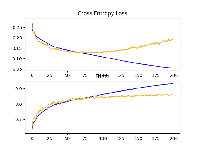
Line Plots Showing Loss and F-Beta Learning Curves for the Baseline Model With Dropout on the Train and Test Datasets on the Planet Problem
Image Data Augmentation
Image data augmentation is a technique that can be used to artificially expand the size of a training dataset by creating modified versions of images in the dataset.
Training deep learning neural network models on more data can result in more skillful models, and the augmentation techniques can create variations of the images that can improve the ability of the fit models to generalize what they have learned to new images.
Data augmentation can also act as a regularization technique, adding noise to the training data and encouraging the model to learn the same features, invariant to their position in the input.
Small changes to the input photos of the satellite photos might be useful for this problem, such as horizontal flips, vertical flips, rotations, zooms, and perhaps more. These augmentations can be specified as arguments to the ImageDataGenerator instance, used for the training dataset. The augmentations should not be used for the test dataset, as we wish to evaluate the performance of the model on the unmodified photographs.
This requires that we have a separate ImageDataGenerator instance for the train and test dataset, then iterators for the train and test sets created from the respective data generators. For example:
|
1 2 3 4 5 6 |
# create data generator train_datagen = ImageDataGenerator(rescale=1.0/255.0, horizontal_flip=True, vertical_flip=True, rotation_range=90) test_datagen = ImageDataGenerator(rescale=1.0/255.0) # prepare iterators train_it = train_datagen.flow(trainX, trainY, batch_size=128) test_it = test_datagen.flow(testX, testY, batch_size=128) |
In this case, photos in the training dataset will be augmented with random horizontal and vertical flips as well as random rotations of up to 90 degrees. Photos in both the train and test steps will have their pixel values scaled in the same way as we did for the baseline model.
The full code listing of the baseline model with training data augmentation for the planet dataset is listed below for completeness.
|
1 2 3 4 5 6 7 8 9 10 11 12 13 14 15 16 17 18 19 20 21 22 23 24 25 26 27 28 29 30 31 32 33 34 35 36 37 38 39 40 41 42 43 44 45 46 47 48 49 50 51 52 53 54 55 56 57 58 59 60 61 62 63 64 65 66 67 68 69 70 71 72 73 74 75 76 77 78 79 80 81 82 83 84 85 86 87 88 89 90 91 92 93 94 95 96 97 98 99 100 101 |
# baseline model with data augmentation for the planet dataset import sys from numpy import load from matplotlib import pyplot from sklearn.model_selection import train_test_split from keras import backend from keras.preprocessing.image import ImageDataGenerator from keras.models import Sequential from keras.layers import Conv2D from keras.layers import MaxPooling2D from keras.layers import Dense from keras.layers import Flatten from keras.optimizers import SGD # load train and test dataset def load_dataset(): # load dataset data = load('planet_data.npz') X, y = data['arr_0'], data['arr_1'] # separate into train and test datasets trainX, testX, trainY, testY = train_test_split(X, y, test_size=0.3, random_state=1) print(trainX.shape, trainY.shape, testX.shape, testY.shape) return trainX, trainY, testX, testY # calculate fbeta score for multi-class/label classification def fbeta(y_true, y_pred, beta=2): # clip predictions y_pred = backend.clip(y_pred, 0, 1) # calculate elements tp = backend.sum(backend.round(backend.clip(y_true * y_pred, 0, 1)), axis=1) fp = backend.sum(backend.round(backend.clip(y_pred - y_true, 0, 1)), axis=1) fn = backend.sum(backend.round(backend.clip(y_true - y_pred, 0, 1)), axis=1) # calculate precision p = tp / (tp + fp + backend.epsilon()) # calculate recall r = tp / (tp + fn + backend.epsilon()) # calculate fbeta, averaged across each class bb = beta ** 2 fbeta_score = backend.mean((1 + bb) * (p * r) / (bb * p + r + backend.epsilon())) return fbeta_score # define cnn model def define_model(in_shape=(128, 128, 3), out_shape=17): model = Sequential() model.add(Conv2D(32, (3, 3), activation='relu', kernel_initializer='he_uniform', padding='same', input_shape=in_shape)) model.add(Conv2D(32, (3, 3), activation='relu', kernel_initializer='he_uniform', padding='same')) model.add(MaxPooling2D((2, 2))) model.add(Conv2D(64, (3, 3), activation='relu', kernel_initializer='he_uniform', padding='same')) model.add(Conv2D(64, (3, 3), activation='relu', kernel_initializer='he_uniform', padding='same')) model.add(MaxPooling2D((2, 2))) model.add(Conv2D(128, (3, 3), activation='relu', kernel_initializer='he_uniform', padding='same')) model.add(Conv2D(128, (3, 3), activation='relu', kernel_initializer='he_uniform', padding='same')) model.add(MaxPooling2D((2, 2))) model.add(Flatten()) model.add(Dense(128, activation='relu', kernel_initializer='he_uniform')) model.add(Dense(out_shape, activation='sigmoid')) # compile model opt = SGD(lr=0.01, momentum=0.9) model.compile(optimizer=opt, loss='binary_crossentropy', metrics=[fbeta]) return model # plot diagnostic learning curves def summarize_diagnostics(history): # plot loss pyplot.subplot(211) pyplot.title('Cross Entropy Loss') pyplot.plot(history.history['loss'], color='blue', label='train') pyplot.plot(history.history['val_loss'], color='orange', label='test') # plot accuracy pyplot.subplot(212) pyplot.title('Fbeta') pyplot.plot(history.history['fbeta'], color='blue', label='train') pyplot.plot(history.history['val_fbeta'], color='orange', label='test') # save plot to file filename = sys.argv[0].split('/')[-1] pyplot.savefig(filename + '_plot.png') pyplot.close() # run the test harness for evaluating a model def run_test_harness(): # load dataset trainX, trainY, testX, testY = load_dataset() # create data generator train_datagen = ImageDataGenerator(rescale=1.0/255.0, horizontal_flip=True, vertical_flip=True, rotation_range=90) test_datagen = ImageDataGenerator(rescale=1.0/255.0) # prepare iterators train_it = train_datagen.flow(trainX, trainY, batch_size=128) test_it = test_datagen.flow(testX, testY, batch_size=128) # define model model = define_model() # fit model history = model.fit_generator(train_it, steps_per_epoch=len(train_it), validation_data=test_it, validation_steps=len(test_it), epochs=200, verbose=0) # evaluate model loss, fbeta = model.evaluate_generator(test_it, steps=len(test_it), verbose=0) print('> loss=%.3f, fbeta=%.3f' % (loss, fbeta)) # learning curves summarize_diagnostics(history) # entry point, run the test harness run_test_harness() |
Running the example first fits the model, then reports the model performance on the hold out test dataset.
Note: Your results may vary given the stochastic nature of the algorithm or evaluation procedure, or differences in numerical precision. Consider running the example a few times and compare the average outcome.
In this case, we can see a lift in performance of about 0.06 from an F-beta score of about 0.831 for the baseline model to a score of about 0.882 for the baseline model with simple data augmentation. This is a large improvement, larger than we saw with dropout.
|
1 2 |
(28335, 128, 128, 3) (28335, 17) (12144, 128, 128, 3) (12144, 17) > loss=0.103, fbeta=0.882 |
Reviewing the learning curves, we can see that the overfitting has been dramatically impacted. Learning continues well past 100 epochs, although may show signs of leveling out towards the end of the run. The results suggest that further augmentation or other types of regularization added to this configuration may be helpful.
It may be interesting to explore additional image augmentations that may further encourage the learning of features invariant to their position in the input, such as zooms and shifts.
Line Plots Showing Loss and F-Beta Learning Curves for the Baseline Model With Data Augmentation on the Train and Test Datasets on the Planet Problem
Discussion
We have explored two different improvements to the baseline model.
The results can be summarized below, although we must assume some variance in these results given the stochastic nature of the algorithm:
- Baseline + Dropout Regularization: 0.859
- Baseline + Data Augmentation: 0.882
As suspected, the addition of regularization techniques slows the progression of the learning algorithms and reduces overfitting, resulting in improved performance on the holdout dataset. It is likely that the combination of both approaches with a further increase in the number of training epochs will result in further improvements. That is, the combination of both dropout with data augmentation.
This is just the beginning of the types of improvements that can be explored on this dataset. In addition to tweaks to the regularization methods described, other regularization methods could be explored such as weight decay and early stopping.
It may be worth exploring changes to the learning algorithm, such as changes to the learning rate, use of a learning rate schedule, or an adaptive learning rate such as Adam.
Alternate model architectures may also be worth exploring. The chosen baseline model is expected to offer more capacity than may be required for this problem and a smaller model may faster to train and in turn could result in better performance.
How to Use Transfer Learning
Transfer learning involves using all or parts of a model trained on a related task.
Keras provides a range of pre-trained models that can be loaded and used wholly or partially via the Keras Applications API.
A useful model for transfer learning is one of the VGG models, such as VGG-16 with 16 layers that, at the time it was developed, achieved top results on the ImageNet photo classification challenge.
The model is comprised of two main parts: the feature extractor part of the model that is made up of VGG blocks, and the classifier part of the model that is made up of fully connected layers and the output layer.
We can use the feature extraction part of the model and add a new classifier part of the model that is tailored to the planets dataset. Specifically, we can hold the weights of all of the convolutional layers fixed during training and only train new fully connected layers that will learn to interpret the features extracted from the model and make a suite of binary classifications.
This can be achieved by loading the VGG-16 model, removing the fully connected layers from the output-end of the model, then adding the new fully connected layers to interpret the model output and make a prediction. The classifier part of the model can be removed automatically by setting the “include_top” argument to “False“, which also requires that the shape of the input be specified for the model, in this case (128, 128, 3). This means that the loaded model ends at the last max pooling layer, after which we can manually add a Flatten layer and the new classifier fully-connected layers.
The define_model() function below implements this and returns a new model ready for training.
|
1 2 3 4 5 6 7 8 9 10 11 12 13 14 15 16 17 |
# define cnn model def define_model(in_shape=(128, 128, 3), out_shape=17): # load model model = VGG16(include_top=False, input_shape=in_shape) # mark loaded layers as not trainable for layer in model.layers: layer.trainable = False # add new classifier layers flat1 = Flatten()(model.layers[-1].output) class1 = Dense(128, activation='relu', kernel_initializer='he_uniform')(flat1) output = Dense(out_shape, activation='sigmoid')(class1) # define new model model = Model(inputs=model.inputs, outputs=output) # compile model opt = SGD(lr=0.01, momentum=0.9) model.compile(optimizer=opt, loss='binary_crossentropy', metrics=[fbeta]) return model |
Once created, we can train the model as before on the training dataset.
Not a lot of training will be required in this case, as only the new fully connected and output layers have trainable weights. As such, we will fix the number of training epochs at 10.
The VGG16 model was trained on a specific ImageNet challenge dataset. As such, the model expects images to be centered. That is, to have the mean pixel values from each channel (red, green, and blue) as calculated on the ImageNet training dataset subtracted from the input.
Keras provides a function to perform this preparation for individual photos via the preprocess_input() function. Nevertheless, we can achieve the same effect with the image data generator, by setting the “featurewise_center” argument to “True” and manually specifying the mean pixel values to use when centering as the mean values from the ImageNet training dataset: [123.68, 116.779, 103.939].
|
1 2 3 4 |
# create data generator datagen = ImageDataGenerator(featurewise_center=True) # specify imagenet mean values for centering datagen.mean = [123.68, 116.779, 103.939] |
The full code listing of the VGG-16 model for transfer learning on the planet dataset is listed below.
|
1 2 3 4 5 6 7 8 9 10 11 12 13 14 15 16 17 18 19 20 21 22 23 24 25 26 27 28 29 30 31 32 33 34 35 36 37 38 39 40 41 42 43 44 45 46 47 48 49 50 51 52 53 54 55 56 57 58 59 60 61 62 63 64 65 66 67 68 69 70 71 72 73 74 75 76 77 78 79 80 81 82 83 84 85 86 87 88 89 90 91 92 93 94 95 96 97 98 99 |
# vgg16 transfer learning on the planet dataset import sys from numpy import load from matplotlib import pyplot from sklearn.model_selection import train_test_split from keras import backend from keras.layers import Dense from keras.layers import Flatten from keras.optimizers import SGD from keras.applications.vgg16 import VGG16 from keras.models import Model from keras.preprocessing.image import ImageDataGenerator # load train and test dataset def load_dataset(): # load dataset data = load('planet_data.npz') X, y = data['arr_0'], data['arr_1'] # separate into train and test datasets trainX, testX, trainY, testY = train_test_split(X, y, test_size=0.3, random_state=1) print(trainX.shape, trainY.shape, testX.shape, testY.shape) return trainX, trainY, testX, testY # calculate fbeta score for multi-class/label classification def fbeta(y_true, y_pred, beta=2): # clip predictions y_pred = backend.clip(y_pred, 0, 1) # calculate elements tp = backend.sum(backend.round(backend.clip(y_true * y_pred, 0, 1)), axis=1) fp = backend.sum(backend.round(backend.clip(y_pred - y_true, 0, 1)), axis=1) fn = backend.sum(backend.round(backend.clip(y_true - y_pred, 0, 1)), axis=1) # calculate precision p = tp / (tp + fp + backend.epsilon()) # calculate recall r = tp / (tp + fn + backend.epsilon()) # calculate fbeta, averaged across each class bb = beta ** 2 fbeta_score = backend.mean((1 + bb) * (p * r) / (bb * p + r + backend.epsilon())) return fbeta_score # define cnn model def define_model(in_shape=(128, 128, 3), out_shape=17): # load model model = VGG16(include_top=False, input_shape=in_shape) # mark loaded layers as not trainable for layer in model.layers: layer.trainable = False # add new classifier layers flat1 = Flatten()(model.layers[-1].output) class1 = Dense(128, activation='relu', kernel_initializer='he_uniform')(flat1) output = Dense(out_shape, activation='sigmoid')(class1) # define new model model = Model(inputs=model.inputs, outputs=output) # compile model opt = SGD(lr=0.01, momentum=0.9) model.compile(optimizer=opt, loss='binary_crossentropy', metrics=[fbeta]) return model # plot diagnostic learning curves def summarize_diagnostics(history): # plot loss pyplot.subplot(211) pyplot.title('Cross Entropy Loss') pyplot.plot(history.history['loss'], color='blue', label='train') pyplot.plot(history.history['val_loss'], color='orange', label='test') # plot accuracy pyplot.subplot(212) pyplot.title('Fbeta') pyplot.plot(history.history['fbeta'], color='blue', label='train') pyplot.plot(history.history['val_fbeta'], color='orange', label='test') # save plot to file filename = sys.argv[0].split('/')[-1] pyplot.savefig(filename + '_plot.png') pyplot.close() # run the test harness for evaluating a model def run_test_harness(): # load dataset trainX, trainY, testX, testY = load_dataset() # create data generator datagen = ImageDataGenerator(featurewise_center=True) # specify imagenet mean values for centering datagen.mean = [123.68, 116.779, 103.939] # prepare iterators train_it = datagen.flow(trainX, trainY, batch_size=128) test_it = datagen.flow(testX, testY, batch_size=128) # define model model = define_model() # fit model history = model.fit_generator(train_it, steps_per_epoch=len(train_it), validation_data=test_it, validation_steps=len(test_it), epochs=20, verbose=0) # evaluate model loss, fbeta = model.evaluate_generator(test_it, steps=len(test_it), verbose=0) print('> loss=%.3f, fbeta=%.3f' % (loss, fbeta)) # learning curves summarize_diagnostics(history) # entry point, run the test harness run_test_harness() |
Running the example first fits the model, then reports the model performance on the hold out test dataset.
Note: Your results may vary given the stochastic nature of the algorithm or evaluation procedure, or differences in numerical precision. Consider running the example a few times and compare the average outcome.
In this case, we can see that the model achieved an F-beta score of about 0.860, which is better than the baseline model, but not as good as the baseline model with image data augmentation.
|
1 2 |
(28335, 128, 128, 3) (28335, 17) (12144, 128, 128, 3) (12144, 17) > loss=0.152, fbeta=0.860 |
Reviewing the learning curves, we can see that the model fits the dataset quickly, showing strong overfitting within just a few training epochs.
The results suggest that the model could benefit from regularization to address overfitting and perhaps other changes to the model or learning process to slow the rate of improvement.
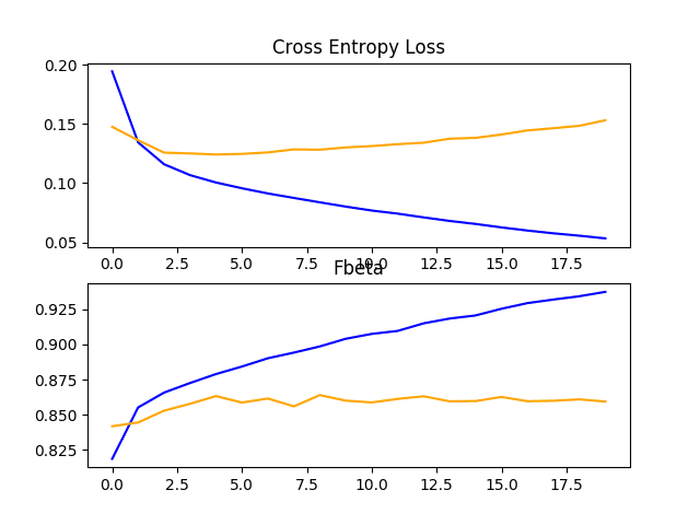
Line Plots Showing Loss and F-Beta Learning Curves for the VGG-16 Model on the Train and Test Datasets on the Planet Problem
The VGG-16 model was designed to classify photographs of objects into one of 1,000 categories. As such, it was designed to pick out fine-grained features of objects. We can guess that the features learned by the model by the deeper layers will represent higher order features seen in the ImageNet dataset that may not be directly relevant to the classification of satellite photos of the Amazon rainforest.
To address this, we can re-fit the VGG-16 model and allow the training algorithm to fine tune the weights for some of the layers in the model. In this case, we will make the three convolutional layers (and pooling layer for consistency) as trainable. The updated version of the define_model() function is listed below.
|
1 2 3 4 5 6 7 8 9 10 11 12 13 14 15 16 17 18 19 20 21 |
# define cnn model def define_model(in_shape=(128, 128, 3), out_shape=17): # load model model = VGG16(include_top=False, input_shape=in_shape) # mark loaded layers as not trainable for layer in model.layers: layer.trainable = False # allow last vgg block to be trainable model.get_layer('block5_conv1').trainable = True model.get_layer('block5_conv2').trainable = True model.get_layer('block5_conv3').trainable = True model.get_layer('block5_pool').trainable = True # add new classifier layers flat1 = Flatten()(model.layers[-1].output) class1 = Dense(128, activation='relu', kernel_initializer='he_uniform')(flat1) output = Dense(out_shape, activation='sigmoid')(class1) # define new model model = Model(inputs=model.inputs, outputs=output) # compile model opt = SGD(lr=0.01, momentum=0.9) model.compile(optimizer=opt, loss='binary_crossentropy', metrics=[fbeta]) |
The example of transfer learning with VGG-16 on the planet dataset can then be re-run with this modification.
Note: Your results may vary given the stochastic nature of the algorithm or evaluation procedure, or differences in numerical precision. Consider running the example a few times and compare the average outcome.
In this case, we see a lift in model performance as compared to the VGG-16 model feature extraction model used as-is improving the F-beta score from about 0.860 to about 0.879. The score is close to the F-beta score seen with the baseline model with the addition of image data augmentation.
|
1 2 |
(28335, 128, 128, 3) (28335, 17) (12144, 128, 128, 3) (12144, 17) > loss=0.210, fbeta=0.879 |
Reviewing the learning curves, we can see that the model still shows signs of overfitting the training dataset relatively early in the run. The results suggest that perhaps the model could benefit from the use of dropout and/or other regularization methods.
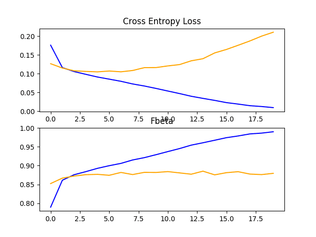
Given that we saw a large improvement with the use of data augmentation on the baseline model, it may be interesting to see if data augmentation can be used to improve the performance of the VGG-16 model with fine-tuning.
In this case, the same define_model() function can be used, although in this case the run_test_harness() can be updated to use image data augmentation as was performed in the previous section. We expect that the addition of data augmentation will slow the rate of improvement. As such we will increase the number of training epochs from 20 to 50 to give the model more time to converge.
The complete example of VGG-16 with fine-tuning and data augmentation is listed below.
|
1 2 3 4 5 6 7 8 9 10 11 12 13 14 15 16 17 18 19 20 21 22 23 24 25 26 27 28 29 30 31 32 33 34 35 36 37 38 39 40 41 42 43 44 45 46 47 48 49 50 51 52 53 54 55 56 57 58 59 60 61 62 63 64 65 66 67 68 69 70 71 72 73 74 75 76 77 78 79 80 81 82 83 84 85 86 87 88 89 90 91 92 93 94 95 96 97 98 99 100 101 102 103 104 105 106 |
# vgg with fine-tuning and data augmentation for the planet dataset import sys from numpy import load from matplotlib import pyplot from sklearn.model_selection import train_test_split from keras import backend from keras.layers import Dense from keras.layers import Flatten from keras.optimizers import SGD from keras.applications.vgg16 import VGG16 from keras.models import Model from keras.preprocessing.image import ImageDataGenerator # load train and test dataset def load_dataset(): # load dataset data = load('planet_data.npz') X, y = data['arr_0'], data['arr_1'] # separate into train and test datasets trainX, testX, trainY, testY = train_test_split(X, y, test_size=0.3, random_state=1) print(trainX.shape, trainY.shape, testX.shape, testY.shape) return trainX, trainY, testX, testY # calculate fbeta score for multi-class/label classification def fbeta(y_true, y_pred, beta=2): # clip predictions y_pred = backend.clip(y_pred, 0, 1) # calculate elements tp = backend.sum(backend.round(backend.clip(y_true * y_pred, 0, 1)), axis=1) fp = backend.sum(backend.round(backend.clip(y_pred - y_true, 0, 1)), axis=1) fn = backend.sum(backend.round(backend.clip(y_true - y_pred, 0, 1)), axis=1) # calculate precision p = tp / (tp + fp + backend.epsilon()) # calculate recall r = tp / (tp + fn + backend.epsilon()) # calculate fbeta, averaged across each class bb = beta ** 2 fbeta_score = backend.mean((1 + bb) * (p * r) / (bb * p + r + backend.epsilon())) return fbeta_score # define cnn model def define_model(in_shape=(128, 128, 3), out_shape=17): # load model model = VGG16(include_top=False, input_shape=in_shape) # mark loaded layers as not trainable for layer in model.layers: layer.trainable = False # allow last vgg block to be trainable model.get_layer('block5_conv1').trainable = True model.get_layer('block5_conv2').trainable = True model.get_layer('block5_conv3').trainable = True model.get_layer('block5_pool').trainable = True # add new classifier layers flat1 = Flatten()(model.layers[-1].output) class1 = Dense(128, activation='relu', kernel_initializer='he_uniform')(flat1) output = Dense(out_shape, activation='sigmoid')(class1) # define new model model = Model(inputs=model.inputs, outputs=output) # compile model opt = SGD(lr=0.01, momentum=0.9) model.compile(optimizer=opt, loss='binary_crossentropy', metrics=[fbeta]) return model # plot diagnostic learning curves def summarize_diagnostics(history): # plot loss pyplot.subplot(211) pyplot.title('Cross Entropy Loss') pyplot.plot(history.history['loss'], color='blue', label='train') pyplot.plot(history.history['val_loss'], color='orange', label='test') # plot accuracy pyplot.subplot(212) pyplot.title('Fbeta') pyplot.plot(history.history['fbeta'], color='blue', label='train') pyplot.plot(history.history['val_fbeta'], color='orange', label='test') # save plot to file filename = sys.argv[0].split('/')[-1] pyplot.savefig(filename + '_plot.png') pyplot.close() # run the test harness for evaluating a model def run_test_harness(): # load dataset trainX, trainY, testX, testY = load_dataset() # create data generator train_datagen = ImageDataGenerator(featurewise_center=True, horizontal_flip=True, vertical_flip=True, rotation_range=90) test_datagen = ImageDataGenerator(featurewise_center=True) # specify imagenet mean values for centering train_datagen.mean = [123.68, 116.779, 103.939] test_datagen.mean = [123.68, 116.779, 103.939] # prepare iterators train_it = train_datagen.flow(trainX, trainY, batch_size=128) test_it = test_datagen.flow(testX, testY, batch_size=128) # define model model = define_model() # fit model history = model.fit_generator(train_it, steps_per_epoch=len(train_it), validation_data=test_it, validation_steps=len(test_it), epochs=50, verbose=0) # evaluate model loss, fbeta = model.evaluate_generator(test_it, steps=len(test_it), verbose=0) print('> loss=%.3f, fbeta=%.3f' % (loss, fbeta)) # learning curves summarize_diagnostics(history) # entry point, run the test harness run_test_harness() |
Running the example first fits the model, then reports the model performance on the hold out test dataset.
Note: Your results may vary given the stochastic nature of the algorithm or evaluation procedure, or differences in numerical precision. Consider running the example a few times and compare the average outcome.
In this case, we can see yet another further lift in model performance from an F-beta score of about 0.879 to an F-beta score of about 0.891.
|
1 2 |
(28335, 128, 128, 3) (28335, 17) (12144, 128, 128, 3) (12144, 17) > loss=0.100, fbeta=0.891 |
Reviewing the learning curves, we can see that data augmentation again has had a large impact on model overfitting, in this case stabilizing the learning and delaying overfitting perhaps until epoch 20.
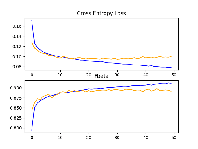
Line Plots Showing Loss and F-Beta Learning Curves for the VGG-16 Model With fine-tuning and Data Augmentation on the Train and Test Datasets on the Planet Problem
Discussion
We have explored three different cases of transfer learning in this section
The results can be summarized below, although we must assume some variance in these results given the stochastic nature of the learning algorithm:
- VGG-16 Model: 0.860.
- VGG-16 Model + fine-tuning: 0.879.
- VGG-16 Model + fine-tuning + Data Augmentation: 0.891.
The choice of the VGG-16 model was somewhat arbitrary, given that it is a smaller and well-understood model. Other models could be used as the basis for transfer learning, such as ResNet, that may achieve better performance.
Further, more fine-tuning may also result in better performance. This might include tuning the weights of more of the feature extractor layers, perhaps with a smaller learning rate. This might also include the modification of the model to add regularization, such as dropout.
How to Finalize the Model and Make Predictions
The process of model improvement may continue for as long as we have ideas and the time and resources to test them out.
At some point, a final model configuration must be chosen and adopted. In this case, we will keep things simple and use the VGG-16 transfer learning, fine-tuning, and data augmentation as the final model.
First, we will finalize our model by fitting a model on the entire training dataset and saving the model to file for later use. We will then load the saved model and use it to make a prediction on a single image.
Save Final Model
The first step is to fit a final model on the entire training dataset.
The load_dataset() function can be updated to no longer split the loaded dataset into train and test sets.
|
1 2 3 4 5 6 |
# load train and test dataset def load_dataset(): # load dataset data = load('planet_data.npz') X, y = data['arr_0'], data['arr_1'] return X, y |
The define_model() function can be used as was defined in the previous section for the VGG-16 model with fine-tuning and data augmentation.
|
1 2 3 4 5 6 7 8 9 10 11 12 13 14 15 16 17 18 19 20 21 22 |
# define cnn model def define_model(in_shape=(128, 128, 3), out_shape=17): # load model model = VGG16(include_top=False, input_shape=in_shape) # mark loaded layers as not trainable for layer in model.layers: layer.trainable = False # allow last vgg block to be trainable model.get_layer('block5_conv1').trainable = True model.get_layer('block5_conv2').trainable = True model.get_layer('block5_conv3').trainable = True model.get_layer('block5_pool').trainable = True # add new classifier layers flat1 = Flatten()(model.layers[-1].output) class1 = Dense(128, activation='relu', kernel_initializer='he_uniform')(flat1) output = Dense(out_shape, activation='sigmoid')(class1) # define new model model = Model(inputs=model.inputs, outputs=output) # compile model opt = SGD(lr=0.01, momentum=0.9) model.compile(optimizer=opt, loss='binary_crossentropy') return model |
Finally, we only require a single data generator and a single iterator for the training dataset.
|
1 2 3 4 5 6 |
# create data generator datagen = ImageDataGenerator(featurewise_center=True, horizontal_flip=True, vertical_flip=True, rotation_range=90) # specify imagenet mean values for centering datagen.mean = [123.68, 116.779, 103.939] # prepare iterator train_it = datagen.flow(X, y, batch_size=128) |
The model will be fit for 50 epochs, after which it will be saved to an H5 file via a call to the save() function on the model
|
1 2 3 4 |
# fit model model.fit_generator(train_it, steps_per_epoch=len(train_it), epochs=50, verbose=0) # save model model.save('final_model.h5') |
Note: saving and loading a Keras model requires that the h5py library is installed on your workstation.
The complete example of fitting the final model on the training dataset and saving it to file is listed below.
|
1 2 3 4 5 6 7 8 9 10 11 12 13 14 15 16 17 18 19 20 21 22 23 24 25 26 27 28 29 30 31 32 33 34 35 36 37 38 39 40 41 42 43 44 45 46 47 48 49 50 51 52 53 54 55 56 57 58 |
# save the final model to file from numpy import load from keras.preprocessing.image import ImageDataGenerator from keras.applications.vgg16 import VGG16 from keras.models import Model from keras.layers import Dense from keras.layers import Flatten from keras.optimizers import SGD # load train and test dataset def load_dataset(): # load dataset data = load('planet_data.npz') X, y = data['arr_0'], data['arr_1'] return X, y # define cnn model def define_model(in_shape=(128, 128, 3), out_shape=17): # load model model = VGG16(include_top=False, input_shape=in_shape) # mark loaded layers as not trainable for layer in model.layers: layer.trainable = False # allow last vgg block to be trainable model.get_layer('block5_conv1').trainable = True model.get_layer('block5_conv2').trainable = True model.get_layer('block5_conv3').trainable = True model.get_layer('block5_pool').trainable = True # add new classifier layers flat1 = Flatten()(model.layers[-1].output) class1 = Dense(128, activation='relu', kernel_initializer='he_uniform')(flat1) output = Dense(out_shape, activation='sigmoid')(class1) # define new model model = Model(inputs=model.inputs, outputs=output) # compile model opt = SGD(lr=0.01, momentum=0.9) model.compile(optimizer=opt, loss='binary_crossentropy') return model # run the test harness for evaluating a model def run_test_harness(): # load dataset X, y = load_dataset() # create data generator datagen = ImageDataGenerator(featurewise_center=True, horizontal_flip=True, vertical_flip=True, rotation_range=90) # specify imagenet mean values for centering datagen.mean = [123.68, 116.779, 103.939] # prepare iterator train_it = datagen.flow(X, y, batch_size=128) # define model model = define_model() # fit model model.fit_generator(train_it, steps_per_epoch=len(train_it), epochs=50, verbose=0) # save model model.save('final_model.h5') # entry point, run the test harness run_test_harness() |
After running this example you will now have a large 91-megabyte file with the name ‘final_model.h5’ in your current working directory.
Make a Prediction
We can use our saved model to make a prediction on new images.
The model assumes that new images are color, and that they have been split into squares with the size of 256×256.
Below is an image extracted from the training dataset, specifically the file train_1.jpg.
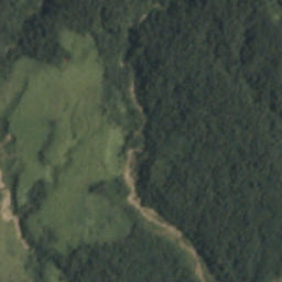
Sample Satellite Image of Amazon Rain Forest For Prediction
Copy it from your training data directory to the current working directory with the name “sample_image.jpg“, for example:
|
1 |
cp train-jpg/train_1.jpg ./sample_image.jpg |
According to the mapping file for the training dataset, this file has the tags (in no specific order):
- agriculture
- clear
- primary
- water
We will pretend this is an entirely new and unseen image, prepared in the required way, and see how we might use our saved model to predict the tags that the image represents.
First, we can load the image and force it to the size to be 128×128 pixels. The loaded image can then be resized to have a single sample in a dataset. The pixel values must also be centered to match the way that the data was prepared during the training of the model.
The load_image() function implements this and will return the loaded image ready for classification.
|
1 2 3 4 5 6 7 8 9 10 11 12 |
# load and prepare the image def load_image(filename): # load the image img = load_img(filename, target_size=(128, 128)) # convert to array img = img_to_array(img) # reshape into a single sample with 3 channels img = img.reshape(1, 128, 128, 3) # center pixel data img = img.astype('float32') img = img - [123.68, 116.779, 103.939] return img |
Next, we can load the model as in the previous section and call the predict() function to predict the content in the image.
|
1 2 |
# predict the class result = model.predict(img) |
This will return a 17-element vector with floating point values between 0 and 1 that could be interpreted as probabilities of the model’s confidence that the photo could be tagged with each known tag.
We can round these probabilities to either 0 or 1 and then use our reverse mapping prepared back in the first section in the create_tag_mapping() function to convert the vector indexes that have a “1” value to tags for the image.
The prediction_to_tags() function below implements this, taking the inverse mapping of integers to tags and the vector predicted by the model for the photo and returning a list of predicted tags.
|
1 2 3 4 5 6 7 |
# convert a prediction to tags def prediction_to_tags(inv_mapping, prediction): # round probabilities to {0, 1} values = prediction.round() # collect all predicted tags tags = [inv_mapping[i] for i in range(len(values)) if values[i] == 1.0] return tags |
We can tie all of this together and make a prediction for the new photo. The complete example is listed below.
|
1 2 3 4 5 6 7 8 9 10 11 12 13 14 15 16 17 18 19 20 21 22 23 24 25 26 27 28 29 30 31 32 33 34 35 36 37 38 39 40 41 42 43 44 45 46 47 48 49 50 51 52 53 54 55 56 57 58 59 60 61 62 63 64 65 |
# make a prediction for a new image from pandas import read_csv from keras.preprocessing.image import load_img from keras.preprocessing.image import img_to_array from keras.models import load_model # create a mapping of tags to integers given the loaded mapping file def create_tag_mapping(mapping_csv): # create a set of all known tags labels = set() for i in range(len(mapping_csv)): # convert spaced separated tags into an array of tags tags = mapping_csv['tags'][i].split(' ') # add tags to the set of known labels labels.update(tags) # convert set of labels to a list to list labels = list(labels) # order set alphabetically labels.sort() # dict that maps labels to integers, and the reverse labels_map = {labels[i]:i for i in range(len(labels))} inv_labels_map = {i:labels[i] for i in range(len(labels))} return labels_map, inv_labels_map # convert a prediction to tags def prediction_to_tags(inv_mapping, prediction): # round probabilities to {0, 1} values = prediction.round() # collect all predicted tags tags = [inv_mapping[i] for i in range(len(values)) if values[i] == 1.0] return tags # load and prepare the image def load_image(filename): # load the image img = load_img(filename, target_size=(128, 128)) # convert to array img = img_to_array(img) # reshape into a single sample with 3 channels img = img.reshape(1, 128, 128, 3) # center pixel data img = img.astype('float32') img = img - [123.68, 116.779, 103.939] return img # load an image and predict the class def run_example(inv_mapping): # load the image img = load_image('sample_image.jpg') # load model model = load_model('final_model.h5') # predict the class result = model.predict(img) print(result[0]) # map prediction to tags tags = prediction_to_tags(inv_mapping, result[0]) print(tags) # load the mapping file filename = 'train_v2.csv' mapping_csv = read_csv(filename) # create a mapping of tags to integers _, inv_mapping = create_tag_mapping(mapping_csv) # entry point, run the example run_example(inv_mapping) |
Running the example first loads and prepares the image, loads the model, and then makes a prediction.
First, the raw 17-element prediction vector is printed. If we wish, we could pretty-print this vector and summarize the predicted confidence that the photo would be assigned each label.
Next, the prediction is rounded and the vector indexes that contain a 1 value are reverse-mapped to their tag string values. The predicted tags are then printed. we can see that the model has correctly predicted the known tags for the provided photo.
It might be interesting to repeat this test with an entirely new photo, such as a photo from the test dataset, after you have already manually suggested tags.
|
1 2 3 4 5 6 |
[9.0940112e-01 3.6541668e-03 1.5959743e-02 6.8241461e-05 8.5694155e-05 9.9828100e-01 7.4096164e-08 5.5998818e-05 3.6668104e-01 1.2538023e-01 4.6371704e-04 3.7660234e-04 9.9999273e-01 1.9014676e-01 5.6060363e-04 1.4613305e-03 9.5227945e-01] ['agriculture', 'clear', 'primary', 'water'] |
Extensions
This section lists some ideas for extending the tutorial that you may wish to explore.
- Tune Learning Rate. Explore changes to the learning algorithm used to train the baseline model, such as alternate learning rate, a learning rate schedule, or an adaptive learning rate algorithm such as Adam.
- Regularize Transfer Learning Model. Explore the addition of further regularization techniques to the transfer learning such as early stopping, dropout, weight decay, and more and compare results.
- Test-Time Automation. Update the model to use test-time prediction, such as flips, rotations, and/or crops to see if prediction performance on the test dataset can be further improved.
If you explore any of these extensions, I’d love to know.
Post your findings in the comments below.
Further Reading
This section provides more resources on the topic if you are looking to go deeper.
API
- Keras image utils source code.
- Keras Applications API
- Keras Image Processing API
- Keras Sequential Model API
- sklearn.metrics.fbeta_score.html API
- sklearn.model_selection.train_test_split API
- Old version of Keras metrics source code (with fbeta_score).
- F-beta score for Keras, Kaggle Kernel.
Articles
- Planet: Understanding the Amazon from Space, Kaggle Competition.
- Download the Planet Dataset, Kaggle.
- Planet Competition Model Evaluation, Kaggle.
- Planet: Understanding the Amazon from Space, 1st Place Winner’s Interview, 2017.
- F1 score, Wikipedia
- Precision and recall, Wikipedia.
Summary
In this tutorial, you discovered how to develop a convolutional neural network to classify satellite photos of the Amazon tropical rainforest.
Specifically, you learned:
- How to load and prepare satellite photos of the Amazon tropical rainforest for modeling.
- How to develop a convolutional neural network for photo classification from scratch and improve model performance.
- How to develop a final model and use it to make ad hoc predictions on new data.
Do you have any questions?
Ask your questions in the comments below and I will do my best to answer.
Develop Deep Learning Models for Vision Today!

Develop Your Own Vision Models in Minutes
...with just a few lines of python code
Discover how in my new Ebook:
Deep Learning for Computer Vision
It provides self-study tutorials on topics like:
classification, object detection (yolo and rcnn), face recognition (vggface and facenet), data preparation and much more...
Finally Bring Deep Learning to your Vision Projects
Skip the Academics. Just Results.


")


How to make segmentation with classification I mean giving color for every class within predicting image this will be more useful and really thank you for your clear tutorial
You can use the Mask RCNN model, described in this book:
https://machinelearningmastery.com/deep-learning-for-computer-vision/
Great stuff, Jason! Many thanks
Thanks Greg!
Dear Jason;
Many thanks for great tutorial.
Is it possible to run the code using .tif file format instead of .jpg?
Could you please guide how to run the .tif format with coordinate system?
For transfer learning, do we need to separate the pre-train, training and validation sets?
Sorry, I don’t have an example of working with TIFF files.
It is a good idea to have separate datasets for train/test/val in general.
when try to plot the first 9 images in my satellite images folder which i prepared it and type my folder path ‘C:/Users/SHAHEEN/Desktop/data/train/train0.jpg’ it says FileNotFoundError: [Errno 2] No such file or directory
Ensure you have downloaded the dataset and unzipped it unto your current working directory.
Amazing Jason, really amazing.
Thanks!
Hi Jason,
Thank you for your post. Is there a reason not using the preprocess_input() function from Keras?
Great question, you can and perhaps should for a standalone application, but we achieve the same effect whilst also training with data augmentation.
Hi Jason,
When I click on the links to download the photos, I get a blank page. Any ideas as to why this happens?
Is this on Kaggle?
https://www.kaggle.com/c/planet-understanding-the-amazon-from-space/data
Does the download begin?
Incredible article!
I wonder, if you play with different models, could it be a time saving trick, if the data is generated only once using the generator and saved as binary matrix. I would guess, the generators generate the data on the fly and processes the same operation each time for each model. Or is the time used by the generators negligible short compared to the calculation-time of the CNN?
Thanks.
I don’t follow, what do you mean by generators in this post?
Hi Jason,
Thank you so much for the great tutorial. I am running the model development code on AWS p3.2x large instance with “Deep Learning AMI (Amazon Linux)” as suggested by you. But I am getting an error mentioned below:
Error: Attempting to fetch value instead of handling error Internal: no supported devices found for platform CUDA
Please suggest what could be the issue.
Thanks,
Aditya
That is very odd, I have not seen that before.
Perhaps confirm you chose an environment correctly (source tensorflow…)?
Perhaps try a new instance?
Perhaps contact AWS support?
I cannot download the dataset. the download button is not showing at all when I hover the mouse over the test-jpg.tar.7z
You must login to Kaggle first.
i already logged in but it still doesn’t show any download option
Try clicking on the file.
You have to accept the rules for this competition
Yes.
Those who are getting the download options over the file, please join Submission first than download button will appear on the file
Thanks for the tip.
I am getting an error while trying for a prediction:
ValueError: Unknown metric function:fbeta
The function must be in scope of its use. Ensure you have copied all of the code:
https://machinelearningmastery.com/faq/single-faq/why-does-the-code-in-the-tutorial-not-work-for-me
Dear Jason,
I have carefully reviewed every line, copied and ran all your code, but got the same error as Dipanjan did. I then downgraded keras and tensorflow at same version as yours and the prediction part still doesn’t work.
Some folks posted about custom metrics issues on Tensorflow’s github repo and none of them has yet worked. I will keep working on it and keep you posted, but would you please check and see if you defined fbeta as a new class in your code? Thank you!
Sorry to hear that, I expect you have not copied all of the required code.
Try copying the complete code example at the end of the tutorial.
hmmm, so it is not necessary to re-define fbeta or the custom metric as a class, create and pass it in load_model() as an object? Sorry for bothering you, I am asking cause Keras documents is using an OOP-approach demo, and some people on github is telling me to rewrite
“model = load_model(‘final_model.h5’)”
to
“model = load_model(‘final_model.h5’, custom_objects={‘fbeta’:fbeta})”, but i tried it and doesn’t work either.
Thank you!
The model is not saved with fbeta metric defined, therefore you don’t need it defined when loading the model and you don’t need the custom_objects argument.
See the section titled “Save Final Model”.
Nvm, i finally figured it out. I bought 4 pdf of yours so far and they are as amazing as this tutorial! I did most of deep learning projects with text analysis but learned so much about image processing from this. Thank you!
Thanks, I’m happy to hear that you have resolved your problem!
I’m not clear as to why the numeric tag values of 0-17 must be on-hot-encoded instead of fed as they are. Can anyone help me understand? thanks
Do you mean for the class labels?
It helps with the framing of the problem and training of the model vial cross entropy.
For more on one hot encoding, see this post:
https://machinelearningmastery.com/why-one-hot-encode-data-in-machine-learning/
yes, sorry…the class labels…since they are already label encoded. Thank you for your response and resource!
No problem.
in this step here:
photo = load_img(filename, target_size = (128,128))should the first argument not be to a file or file path instead of the csv?
Also, shouldn’t this be : tags = create_file_mappings? I’m a bit lost on this line of code.
tags = file_mapping(filename[:-4])
is filename calling just one key from the dict? and is the -4 just for illustration?
Yes, filename references an image. Check the load_dataset() function.
I’m also curious about the second part of matan’s question… it says tags = file_mapping, but should this be create_file_mapping? there is no define file_mapping ?
It retrieves the filename without the file extension.
this also comes up in several instances aftewards, file_mapping is not defined, is it supposed to be create_file_mapping ?
ahh okay that was dumb, makes sense… my only problem is now when i run that line of code :
tags = file_mapping[filename[:-4]]
I receive a KeyError:’FILENAME’ …
any idea as to why this is happening ?
Hi Jason
very interesting post.
You mention: “In this case, we are working neither with a binary or multi-class classification task; instead, it is a multi-label classification task and the number of labels are not balanced, with some used more heavily than others.”
My question now, is balancing not needed?
(For multi-class problems this typically needs to be done.)
Yes, it is a good idea to have some balance in the observed labels if possible.
This is not always possible. You can look at what types of errors are made by your model and if they are mostly around a specific label, you can look into using data augmentation or over/under sampling methods to better express that label in the training dataset.
Hi Jason
thanks for your reply.
I was looking for some papers and discussions in stackoverflow etc. and found that class balancing for multilabel classification is not as straight forward as for the multiclass problem..
E.g here
https://stackoverflow.com/questions/48485870/multi-label-classification-with-class-weights-in-keras
or here
https://www.researchgate.net/publication/278699395_Managing_Imbalanced_Data_Sets_in_Multi-label_Problems_A_Case_Study_with_the_SMOTE_Algorithm
do you mean this with “This is not always possible”?
SMOTE is very effective for tabular datasets. I don’t know about its use in computer vision, I would expect data augmentation is used instead.
It’s a wonderful question. I believe research/experimentation may be required to get a good answer.
thanks! given lack of time I will do some “heuristic” balancing approach
what is the effect of the extra indentation before validation here?
history = model.fit_generator(train_it, steps_per_epoch=len(train_it),
validation_data=test_it, validation_steps=len(test_it), epochs=50, verbose=0)
That is one long line that I wrapped onto two lines.
thank you Sir!
how can we get loss and Fbeta to print out after each epoch to see progress but mostly to confirm the model is running? I’m using a google cloud engine instance with 16cpu and 64gb memory and the baseline with dropout, 200 epochs has been running for over 12 hours.
verbose=1
Hi Jason, great post. I’m trying to do something similar with 200 classes. Starting with a really low fbeta ~ 0.03 (basically what it would be if they were all zeroes or all ones). label sets are reasonably balanced but can’t seem to make progress no matter what I try with augmentation, dropout, more/less dense layers, different optimisers. Any suggestions would be great
Hmmm, try this checklist:
https://machinelearningmastery.com/improve-deep-learning-performance/
Try the ideas here:
https://machinelearningmastery.com/start-here/#better
Hi, first thanks for the awesome post, I tried to adapt this example and try out InceptionResnet-v2 (same dataset), retraining the last six layers and adding the same classification layers of this example, my loss in training is always around 0.7 to 0.1, and in validation always higher than 1 (goes up to 10), (fbeta scores are similar though for train and validation), is my model overfitting and how are my fbeta scores similar for train and validation when my loss values are significantly different (for train and val) ?
It sounds like it is overfitting, see this to be sure:
https://machinelearningmastery.com/learning-curves-for-diagnosing-machine-learning-model-performance/
Only look at loss to see if you are overfitting. fbeta is just the metric you are using to evaluate the model. loss tells you about learning dynamics.
Hi
I have multi-label image classification problem where I have a total of 3 labels (Label1, Label2, Label3) and each label further have 3 options (L, M, H)
How we can encode this type of scenario, so we can use it for training?
One hot encoding.
Please correct me if I am wrong
As I mentioned each label have further 3 attributes (L, M, H)
Suppose we have 3 inputs (001, 002 & 003)
and against each input, we have vector y which will look like
X Y encoded values
001 -> [L, M,L ] -> [ [1,0,0], [0,1,0], [1,0,0] ]
002 -> [H, M,L ] -> [ [0,0,1], [0,1,0], [1,0,0] ]
003 -> [H, H,H ] -> [ [0,0,1], [0,0,1], [0,0,1] ]
am I right?
and on the final layer, there will be a total of 9 neurons
like model.add(Dense(9,activation=’sigmoid’) ?
Not sure I follow at first glance. Perhaps test it and see?
I encoded all labels in this way
001 -> [L, M,L ] -> [ [1,0,0], [0,1,0], [1,0,0] ]
002 -> [H, M,L ] -> [ [0,0,1], [0,1,0], [1,0,0] ]
created a neural network and
on the last layer, I used this
model.add(Dense(5))
model.add(Reshape( (5, 3) ))
model.add(Activation(‘softmax’))
“InvalidArgumentError: Input to reshape is a tensor with 100 values, but the requested shape has 300”
I think you want a Dense with 3 nodes given you are predicting the probability for 3 class labels.
e.g.
Actually just for an idea, I used 3 labels in above comment in actually I have total 5 labels and each label have further 3 (L, M, H) attributes
Yeah I tried
model.add(Dense(5,activation=’softmax’))
but still facing issue don’t know what’s going wrong
“InvalidArgumentError: logits and labels must be broadcastable: logits_size=[15,5] labels_size=[45,5]”
Can you please take a look here
https://drive.google.com/open?id=156Ic6g-Ldcfy0q5B5tdQuZvTKm-xuFPh
I will very thankful to you because I am stuck here from a couple of days
If I use
model.add(Dense(5,activation=’sigmoid’))
then I faced
“InvalidArgumentError: Incompatible shapes: [15,5] vs. [15]”
If you have 5 classes, ensure that you are using categorical cross entropy loss and that you have one hot encoded the class labels.
Hi
I need a confirmation that either I am going in the right direction or not
Below is detail
Scenario
I have multi-label image classification problem where I have a total of 5 labels (Label1, Label2, Label3, Label4, and Label5) and each label further have 3 options (L, M, H)
Actually against each Labels (Label1, Label2, Label3, Label4, and Label5), I got a numeric value like
Label1 —-> 5
Label2 —-> 90
Label3 —-> 30
Label4 —-> 20
Label5 —-> 67
I convert above numeric value into category For example If the value
0 – 33 —– I assigned ‘L’
34 – 66 —– I assigned ‘M;
67 – 100 — I assigned ‘H’
and My CSV file is like
Id Labels
001-01-01 L M L L M
001-01-02 M M H H H
001-01-03 L L L L M
.
.
.
.
300-01-15 M L M L H
In my CSV, against Id, I have the image in the images folder.
So First I convert above labels into one-hot encoded like
001-01-01 -> [L, M,L ] -> [ [1,0,0], [0,1,0], [1,0,0] ]
001-01-02 -> [H, M,L ] -> [ [0,0,1], [0,1,0], [1,0,0] ]
then I created CNN and pass images to network
My final layer is like
model.add(Dense(15))
model.add(Reshape((5,3)))
model.add(Activation(‘softmax’))
This is the right way to solve this kind of problem
I did R&D but couldn’t find solution like this that’s why need confirmation because I am a beginner in this field
I’m not sure the approach is sound.
It sounds like a multi-label classification with 5 classes, and each label has 3 mutually exclusive labels.
If the labels were binary, the above tutorial would be a good fit. Instead, a different approach is required and perhaps some trial and error to figure out the best approach to encode the labels.
Off the cuff I don’t many good ideas, perhaps a multi-output model with a one hot encoding for each class – that’s the first sensible idea that comes to me.
Hi
Accoding to my problem (as I mentioned above), I did hot encoding in this way
I convert above numeric value into category For example If the value
0 – 33 —– I assigned ‘L’
34 – 66 —– I assigned ‘M;
67 – 100 — I assigned ‘H’
and My CSV file is like
Id ————- > Labels
001-01-01 ————- > L M L L M
001-01-02 ————- > M M H H H
001-01-03 ————- > L L L L M
In my CSV, against Id, I have the image in the images folder.
So First I convert above labels into one-hot encoded like
001-01-01 -> [L, M,L ] -> [ [1,0,0], [0,1,0], [1,0,0] ]
001-01-02 -> [H, M,L ] -> [ [0,0,1], [0,1,0], [1,0,0] ]
then I created CNN and pass images to network
My final layer is like
model.add(Dense(15))
model.add(Reshape((5,3)))
model.add(Activation(‘softmax’))
I did follow above tutorial for this implementation and I saw I achived
loss: 5.9617 – acc: 0.6124 (In case of training and validation)
but In above tutorial loss was also in (0.something) but In my case is 5.something
I am confuse in accuracy measurement.
Please let me know how we can and what is correct way
Perhaps try alternate configuration of the model?
Perhaps try alternate configuration of the optimizer?
Perhaps try alternate models?
Perhaps try alternate preparation of the data?
More suggestions here:
https://machinelearningmastery.com/start-here/#better
Hi
I have one query regarding the performance of the model
As you mentioned in this tutorial your model achieved loss=0.100, fbeta=0.891
it’s mean your model achieved 89% accuracy?
Please let me know about it what does this mean
as in my case
model.compile(loss=’binary_crossentropy’, optimizer=’adam’, metrics=[‘accuracy’])
loss: 0.5700 – acc: 0.7031 – val_loss: 0.5643 – val_acc: 0.6850
what does this mean?
No, fbeta is not accuracy. More on fbeta here:
https://en.wikipedia.org/wiki/F1_score
Hi Jason,
My dataset includes different formated images: png and tif. All dataset should be same format for getting better accuracy during training or format doesn’t effect too much?
How image formats such as jpeg,png,tif etc. differ in model’s accuracy?
Thank you for your all posts, very helpful!
Once you have the pixels loaded in memory it probably doesn’t make any difference.
Hey Jason,
About the previous fbeta customized metric problem that I asked, may I please know if I need to define a “fbeta” variable from the “fbeta(y_true, y_pred, beta=2)” function by myself, such as:
fbeta = fbeta(y_true, y_pred, beta=2)
or calling the function when I compile the model? if so, what exactly should I pass in the fbeta function for y_true and y_predict, when defining fbeta while compiling the model?
I really want to know this because I also noticed that in this tutorial, the only times when you called fbeta function manually was when you use to demo how keras and sklearn yield same train and test scores for all ones. I think i have the correct functions and code but missing a line to define or call fbeta properly, before making the model’s prediction.
Thank you!
Bbeta is only needed when evaluating the model.
The final model should not be saved with the fbeta metric defined. As such, when you load it, you do not need the fbeta metric defined and used.
If you do want to save/load the model with the fbeta metric, then ust the custom_objects argument in the load_model() function and ensure the function is defined prior to this call.
Thanks for this tutorial Jason. I am seeing something crazy while working with this. My training loss first decreases and then starts increasing after the 8th epoch. This should definitely not happen with training data. Any tips on how to diagnose the issue? thanks!
You’re welcome.
This may help with diagnostic tools:
https://machinelearningmastery.com/start-here/#better
Specifically this:
https://machinelearningmastery.com/learning-curves-for-diagnosing-machine-learning-model-performance/
Hello Jason this is an amazing read. May I know how do metrics count the number of “correct” predictions in these image-wise classifications? Does a prediction has to be 100% matching the human-generated labels to be counted as a correct prediction? For instance if an image in test set has 5 human-generated labels, what if the model (a) predicted 4 out 5 of them or (b) predicted 7 labels, 5 of them are correct, with 2 extra ones (c) predicted 7 labels, 4 of them are correct but 3 of them are incorrect? Thank you!
Accuracy is calculated as total correct predictions divided by the total number of predictions made.
– 4/5 is 0.8 or 80% correct.
– 5/7 is is about 0.71 or 71% correct.
Does that help?
Jason, my apology as I wasn’t being clear enough. I guess my question was “In image-wise classifications, should we give our model ‘partial credits’ if it gets some of the labels correctly in a single image prediction”. I will use this made-up test set of 3 images as an example:
Image0 | Labels: A, B, C, D | Model Predictions: A, B, C, D
Image1 | Labels: B, G, H, M | Model Predictions: B, C, G, H
Image2 | Labels: A, D, F | Model Predictions: A, D, F, K
Would you consider this as 1/3 = 33% correct, since only 1 out of 3 images is predicted EXACTLY identical with the manually-tagged labels?
Should we completely neglect the attempts with Image1 and Image2? In Image2, it technically got all the labels but added an extra one, while in Image1, it did not predict all labels correctly.
Thank you!
This happens via the chosen loss function during training.
Yes, you can choose to evaluate predictions on a test set that way.
Hi sir,
Thank you for this wonderful tutorial.
I tried implementing the similar code for MTFL dataset where there are face images and we have three tags “gender”, “smiling”, “wearing glasses”.
When i am trying to do result = model.predict(image) and then print(result), it is giving output as [nan, nan, nan] for any image I run on.
Please help.
That sounds like a cool project!
Sounds like perhaps weights went to nan, overflow or underflow.
Maybe check the loss during training?
Maybe add regularization to the weights?
Maybe Maybe scale inputs?
…
Hello Jason, thanks for helping.
Finally I found that when I remove below four lines, the predictions are being made correct.
If I include these four, then it is giving output [0,0,0] for any image that I predict.
model.get_layer(‘block5_conv1’).trainable = True
model.get_layer(‘block5_conv2’).trainable = True
model.get_layer(‘block5_conv3’).trainable = True
model.get_layer(‘block5_pool’).trainable = True
Please help if you know why this is happening.
I cannot explain your claim.
changing
class1 = Dense(128, activation=’relu’, kernel_initializer=’he_uniform’)(flat1)
to
class1 = Dense(128, activation=’softmax’, kernel_initializer=’he_uniform’)(flat1)
working for me
Thanks for the prompt reply.
A strange thing I am noticing is that when I am running model.predict on the model where we used fbeta matrix(the code just before the “Discussion” section). This is producing the required results.
But, when I am saving the model similar to the one you wrote at the end of the tutorial(“Save final model” section) and then predicting after loading it, it is giving nan values.
What can be the reason behind this?
Perhaps confirm that it was saved and loaded correctly?
Perhaps confirm you copied all of the code?
Perhaps confirm your environment is up to date?
Perhaps try running it all again?
i want to detect diseases i am trying on Alzheimer_s Dataset plz send me code for image classification with single image prediction i have 4 classes pls send code on my email-id
You can get started with image classification tutorials here:
https://machinelearningmastery.com/start-here/#dlfcv
Can you please suggest me how to use tiff images dataset.As i am working on another datset which does not have any other format images except tiff so i am stuck there.Please suggest.
Thank you.
Sorry, I don’t think I have tutorials for working with tiff images, perhaps this give you ideas:
https://machinelearningmastery.com/how-to-load-and-manipulate-images-for-deep-learning-in-python-with-pil-pillow/
Jason, Loved the article. I am coming up the learning curve on Neural Networks and have a very basic question: Can a single NN identify multiple classifications? Since weights and biases on the layers must be adjusted to match sample data, it seems like each time this is done prior adjustments will be destroyed. So it seems to me that a single NN can only identify a single classification. If not, could a single NN identify hundreds of different things? I am hoping you can point me in the right direction to understanding NN limitations.
Thanks!
Yes. The model learns across examples so it can make predictions on any new examples from the domain. Yes, a fit model can be used indefinitely – at least until the problem changes.
Perhaps this will help in understanding how a fit model can be used to make ad hoc predictions:
https://machinelearningmastery.com/how-to-make-classification-and-regression-predictions-for-deep-learning-models-in-keras/
Thank you so much!
You’re welcome.
Hi Jason,
Do you have multilabel classification covered in the computer vision book & codes?
Yes, a version of this example appears in the book.
Hi Jason,
I have bought machine_learning_mastery_with_python, data_preparation_for_machine_learning,
imbalanced-classification-with-python and machine-learning-algorithms-from-scratch
books of yours ..
Could you please let me know where is the Multi-Label Classification Problem example is written? It would be a great help ..
Thanks in advance .. 🙂
Sorry, I don’t have book that covers multi-label classification, I hope to cover the topic in detail in the future.
Hi Jason,
Great tutorial and very inspirational as usual. Thank you.
I did to your transfer learning VGG16 model the following experiments That I share.
I) Minor comments
– I can not use the “stratify” argument on the “train_test_split()” function (more appropriate), because there is not more than one sample per label type.
– In order to be able to load the trained .h5 model defined with our own ‘fbeta’ metric (I compile the model just before saving -at the end of the model fitting-, by removing the fbeta metric parameter). So later one we can load the model without problem
– I apply the “preprocess_input” function to all images to avoid to go trough yours specific values of featurewise center that you provided.
– In order to apply progressive training, even when I do not apply data augmentation, I can use the “ImageDataGenerator()” keras function, but without any argument a t all (empty)…so this, let us apply latter the fit_generator to the input-output model.
– Because we load the keras App VGG16, I also use this full model to predict the satellite Amazonia imaging, just for fun…I got the class “poncho” for the example image!.
II) Experiments
– I replace VGG16 by “Inceptionv3” Keras App, for feature extraction usually with a better imagenet results than VGG16, but for my own surprise I got an insufficient fbeta score = 64.5% . I do not know why.
– I study the results sensitivity vs input pixels image resolution ( 64, 128 and 224) and I got 2% less point for (64,64) pixels images than for (128,128)…but surprisingly with more square pixels (224,224) I got less ‘fbeta’ score than for (128,128). I do not know why. Also working with (224,224) pixels resolution takes 45 minutes to complete one single epoch. Too much time vs 15 minutes for 128, 128 resolution
– I study the results sensitivity vs number of VGG16 layers training (defrosting to brew re-trained according to Amazonia imaging) and I got 4% better when I defrost the whole block5 of VGG16. But also I got “nan” results when I tried to defrost more blocks (e.eg. block4 plus block5) of VGG16 app. I do not know why.
I would like to experiment comparing this Multi-label classification technique vs the Image captioning technique (NLP+ img Feature Extraction) following your image captioning tutorial (but replacing the 5 descriptions for one single description with the corresponding multi-labels words). I guess this simple Multi-label class should perform better.
One more time thank you for yours amazing tutorials.
regards,
JG
Very nice work, thanks for sharing JG!
hello jason, great tutorial, very intuitive.
i am however having issues with mapping the predicted values to tags for a more than one prediction, i keep getting this error.
ValueError: The truth value of an array with more than one element is ambiguous. Use a.any() or a.all()
can you help with a suggestion on how to go about this?
Sorry to hear that, are you able to confirm your Keras and TensorFlow libraries are up to date?
Also these suggestions may help:
https://machinelearningmastery.com/faq/single-faq/why-does-the-code-in-the-tutorial-not-work-for-me
Hello Professor jason
Could you help me how to classify more than one class then based on the classified class, how to classify the class inside this class ?
Sounds like hierarchical classification.
I don’t have an example, but perhaps you can begin experimenting and I can answer more specific questions you have along the way.
Hello Prof.jason, i had finally recognized that my dataset structure is similar to CIFAR-100. But, i don’t know how to load my data? How to split them into training and testing data as CIFAR dataset’s structure?
Could you help me please with some guide if you have not covered this topic in your site?
Thanks in advance.
This will show you how to load each image:
https://machinelearningmastery.com/how-to-load-convert-and-save-images-with-the-keras-api/
This will show you how to load larger datasets:
https://machinelearningmastery.com/how-to-load-large-datasets-from-directories-for-deep-learning-with-keras/
Thanks for the tutorial!
In remote sensing task, we usually ended up with a classified map in different colours that show different classes, but in this case, you just predicted labels, not classify or segments input image into corresponding labels, for example, how should I know the class or label of pixel(i,j) in the input image?
also in remote sensing, you usually work with big scenes with dimensions like 5000*5000. after turning this big scene into 128,128 image chips, how we should get back to our main classified scene(5000*5000). It would be great if you explain that.
Correct, this was a multi-label classification task.
It sounds like you are describing object detection.
I don’t have an example of object detection in satellite images, but perhaps this will help as a starting point:
https://machinelearningmastery.com/how-to-perform-object-detection-in-photographs-with-mask-r-cnn-in-keras/
Hi Jason,
Thank you very much for the great tutorial. I really enjoyed this article. Actually, I am trying to use this multi-label classification example for my own project which is the prediction of 11 classes for images. It is a multi classification problem not a multi-label classification problem. My dataset includes 2428 jpg images. However, in the section where you wanted to create the dataset, for this line “tags = file_mapping[filename[:-4]]” I received an error. I think it is related to the dimension of vectors. I don’t know how to fix it and I really appreciate some help. Also, I am using google Colab for running the code but when I wanted to run the code with Planet dataset on Google Colab, it couldn’t create the npz file which is strange.
I found this article which you suggest to some folks for multi-classification problem:
https://machinelearningmastery.com/how-to-develop-a-cnn-from-scratch-for-cifar-10-photo-classification/
Is this better to start my work, instead of working on multi-label classification problem?
I really appreciate your guidance
You’re welcome.
The code in the above tutorial for loading the dataset is specific to this specific dataset. You must write custom code to load your specific dataset.
whenever i use datagen.mean = [123.68, 116.779, 103.939], and i do print to see value, it’s all become negative .
Perhaps check your code, you may have introduced a bug.
Hallo Professor Jason,
When i tried for the code, i always faced ‘fbeta_score() takes 2 positional arguments but 3 positional arguments (and 1 keyword-only argument) were given’ in Model Evaluation Section.
Would you please any idea for the solution of that error. Thanks
Hi Toto…did you copy and past the code? That could be a contributing factor.
Hi james,
I want to classify my images in three classes (dry, wet and dark)
Below is the code:
# baseline model for the planet dataset
import sys
from numpy import load
from matplotlib import pyplot
from sklearn.model_selection import train_test_split
from keras import backend
from keras.preprocessing.image import ImageDataGenerator
from keras.models import Sequential
from keras.layers import Conv2D
from keras.layers import MaxPooling2D
from keras.layers import Dense
from keras.layers import Flatten
from tensorflow.keras.optimizers import SGD
import tensorflow as tf
# load train and test dataset
def load_dataset():
# load dataset
data = load(‘/Data_set.npz’)
X, y = data[‘arr_0’], data[‘arr_1′]
# separate into train and test datasets
trainX, testX, trainY, testY = train_test_split(X, y, test_size=0.3, random_state=1)
print(trainX.shape, trainY.shape, testX.shape, testY.shape)
return trainX, trainY, testX, testY
# calculate fbeta score for multi-class/label classification
# def fbeta(y_true, y_pred, beta=2):
# # clip predictions
# y_pred = backend.clip(y_pred, 0, 1)
# # calculate elements
# tp = backend.sum(backend.round(backend.clip(y_true * y_pred, 0, 1)), axis=1)
# fp = backend.sum(backend.round(backend.clip(y_pred – y_true, 0, 1)), axis=1)
# fn = backend.sum(backend.round(backend.clip(y_true – y_pred, 0, 1)), axis=1)
# # calculate precision
# p = tp / (tp + fp + backend.epsilon())
# # calculate recall
# r = tp / (tp + fn + backend.epsilon())
# # calculate fbeta, averaged across each class
# bb = beta ** 2
# fbeta_score = backend.mean((1 + bb) * (p * r) / (bb * p + r + backend.epsilon()))
# return fbeta_score
# define cnn model
def define_model(in_shape=(224, 224, 3), out_shape=1):
model = Sequential()
model.add(Conv2D(32, (3, 3), activation=’relu’, kernel_initializer=’he_uniform’, padding=’same’, input_shape=in_shape))
model.add(Conv2D(32, (3, 3), activation=’relu’, kernel_initializer=’he_uniform’, padding=’same’))
model.add(MaxPooling2D((2, 2)))
model.add(Conv2D(64, (3, 3), activation=’relu’, kernel_initializer=’he_uniform’, padding=’same’))
model.add(Conv2D(64, (3, 3), activation=’relu’, kernel_initializer=’he_uniform’, padding=’same’))
model.add(MaxPooling2D((2, 2)))
model.add(Conv2D(128, (3, 3), activation=’relu’, kernel_initializer=’he_uniform’, padding=’same’))
model.add(Conv2D(128, (3, 3), activation=’relu’, kernel_initializer=’he_uniform’, padding=’same’))
model.add(MaxPooling2D((2, 2)))
model.add(Flatten())
model.add(Dense(128, activation=’relu’, kernel_initializer=’he_uniform’))
model.add(Dense(out_shape, activation=’softmax’))
# compile model
opt = SGD(lr=0.01, momentum=0.9)
model.compile(optimizer=opt, loss=’categorical_crossentropy’, metrics=[‘accuracy’])
return model
# plot diagnostic learning curves
def summarize_diagnostics(history):
# plot loss
pyplot.subplot(211)
pyplot.title(‘Cross Entropy Loss’)
pyplot.plot(history.history[‘loss’], color=’blue’, label=’train’)
pyplot.plot(history.history[‘val_loss’], color=’orange’, label=’test’)
# plot accuracy
pyplot.subplot(212)
pyplot.title(‘accuracy’)
pyplot.plot(history.history[‘fbeta’], color=’blue’, label=’train’)
pyplot.plot(history.history[‘val_fbeta’], color=’orange’, label=’test’)
# save plot to file
filename = ‘/gdrive/MyDrive/’
pyplot.savefig(filename + ‘BaseLine_1.png’)
pyplot.close()
# run the test harness for evaluating a model
def run_test_harness():
# load dataset
trainX, trainY, testX, testY = load_dataset()
# create data generator
datagen = ImageDataGenerator(rescale=1.0/255.0)
# prepare iterators
train_it = datagen.flow(trainX, trainY, batch_size=32)
test_it = datagen.flow(testX, testY, batch_size=32)
# define model
model = define_model()
# fit model
history = model.fit_generator(train_it, steps_per_epoch=len(train_it),
validation_data=test_it, validation_steps=len(test_it), epochs=15, verbose=0)
# evaluate model
loss, fbeta = model.evaluate_generator(test_it, steps=len(test_it), verbose=0)
print(‘> loss=%.3f, fbeta=%.3f’ % (loss, fbeta))
# learning curves
summarize_diagnostics(history)
# entry point, run the test harness
run_test_harness()
I had run the code and got no errors but it showing me “loss=0.00 and accuracy=0.000”
what does this mean and what is the problem?
Please help
Sorry it seems too long for me to read and debug your code. But the zero loss and zero accuracy seems contradicting. I would suggest you check the parameters you passed into
compile()function is matching what you intended to do.