Deep learning neural networks are generally opaque, meaning that although they can make useful and skillful predictions, it is not clear how or why a given prediction was made.
Convolutional neural networks, have internal structures that are designed to operate upon two-dimensional image data, and as such preserve the spatial relationships for what was learned by the model. Specifically, the two-dimensional filters learned by the model can be inspected and visualized to discover the types of features that the model will detect, and the activation maps output by convolutional layers can be inspected to understand exactly what features were detected for a given input image.
In this tutorial, you will discover how to develop simple visualizations for filters and feature maps in a convolutional neural network.
After completing this tutorial, you will know:
- How to develop a visualization for specific filters in a convolutional neural network.
- How to develop a visualization for specific feature maps in a convolutional neural network.
- How to systematically visualize feature maps for each block in a deep convolutional neural network.
Kick-start your project with my new book Deep Learning for Computer Vision, including step-by-step tutorials and the Python source code files for all examples.
Let’s get started.
How to Visualize Filters and Feature Maps in Convolutional Neural Networks
Photo by Mark Kent, some rights reserved.
Tutorial Overview
This tutorial is divided into four parts; they are:
- Visualizing Convolutional Layers
- Pre-fit VGG Model
- How to Visualize Filters
- How to Visualize Feature Maps
Visualizing Convolutional Layers
Neural network models are generally referred to as being opaque. This means that they are poor at explaining the reason why a specific decision or prediction was made.
Convolutional neural networks are designed to work with image data, and their structure and function suggest that should be less inscrutable than other types of neural networks.
Specifically, the models are comprised of small linear filters and the result of applying filters called activation maps, or more generally, feature maps.
Both filters and feature maps can be visualized.
For example, we can design and understand small filters, such as line detectors. Perhaps visualizing the filters within a learned convolutional neural network can provide insight into how the model works.
The feature maps that result from applying filters to input images and to feature maps output by prior layers could provide insight into the internal representation that the model has of a specific input at a given point in the model.
We will explore both of these approaches to visualizing a convolutional neural network in this tutorial.
Want Results with Deep Learning for Computer Vision?
Take my free 7-day email crash course now (with sample code).
Click to sign-up and also get a free PDF Ebook version of the course.
Pre-fit VGG Model
We need a model to visualize.
Instead of fitting a model from scratch, we can use a pre-fit prior state-of-the-art image classification model.
Keras provides many examples of well-performing image classification models developed by different research groups for the ImageNet Large Scale Visual Recognition Challenge, or ILSVRC. One example is the VGG-16 model that achieved top results in the 2014 competition.
This is a good model to use for visualization because it has a simple uniform structure of serially ordered convolutional and pooling layers, it is deep with 16 learned layers, and it performed very well, meaning that the filters and resulting feature maps will capture useful features. For more information on this model, see the 2015 paper “Very Deep Convolutional Networks for Large-Scale Image Recognition.”
We can load and summarize the VGG16 model with just a few lines of code; for example:
|
1 2 3 4 5 6 |
# load vgg model from keras.applications.vgg16 import VGG16 # load the model model = VGG16() # summarize the model model.summary() |
Running the example will load the model weights into memory and print a summary of the loaded model.
If this is the first time that you have loaded the model, the weights will be downloaded from the internet and stored in your home directory. These weights are approximately 500 megabytes and may take a moment to download depending on the speed of your internet connection.
We can see that the layers are well named, organized into blocks, and named with integer indexes within each block.
|
1 2 3 4 5 6 7 8 9 10 11 12 13 14 15 16 17 18 19 20 21 22 23 24 25 26 27 28 29 30 31 32 33 34 35 36 37 38 39 40 41 42 43 44 45 46 47 48 49 50 51 52 53 |
_________________________________________________________________ Layer (type) Output Shape Param # ================================================================= input_1 (InputLayer) (None, 224, 224, 3) 0 _________________________________________________________________ block1_conv1 (Conv2D) (None, 224, 224, 64) 1792 _________________________________________________________________ block1_conv2 (Conv2D) (None, 224, 224, 64) 36928 _________________________________________________________________ block1_pool (MaxPooling2D) (None, 112, 112, 64) 0 _________________________________________________________________ block2_conv1 (Conv2D) (None, 112, 112, 128) 73856 _________________________________________________________________ block2_conv2 (Conv2D) (None, 112, 112, 128) 147584 _________________________________________________________________ block2_pool (MaxPooling2D) (None, 56, 56, 128) 0 _________________________________________________________________ block3_conv1 (Conv2D) (None, 56, 56, 256) 295168 _________________________________________________________________ block3_conv2 (Conv2D) (None, 56, 56, 256) 590080 _________________________________________________________________ block3_conv3 (Conv2D) (None, 56, 56, 256) 590080 _________________________________________________________________ block3_pool (MaxPooling2D) (None, 28, 28, 256) 0 _________________________________________________________________ block4_conv1 (Conv2D) (None, 28, 28, 512) 1180160 _________________________________________________________________ block4_conv2 (Conv2D) (None, 28, 28, 512) 2359808 _________________________________________________________________ block4_conv3 (Conv2D) (None, 28, 28, 512) 2359808 _________________________________________________________________ block4_pool (MaxPooling2D) (None, 14, 14, 512) 0 _________________________________________________________________ block5_conv1 (Conv2D) (None, 14, 14, 512) 2359808 _________________________________________________________________ block5_conv2 (Conv2D) (None, 14, 14, 512) 2359808 _________________________________________________________________ block5_conv3 (Conv2D) (None, 14, 14, 512) 2359808 _________________________________________________________________ block5_pool (MaxPooling2D) (None, 7, 7, 512) 0 _________________________________________________________________ flatten (Flatten) (None, 25088) 0 _________________________________________________________________ fc1 (Dense) (None, 4096) 102764544 _________________________________________________________________ fc2 (Dense) (None, 4096) 16781312 _________________________________________________________________ predictions (Dense) (None, 1000) 4097000 ================================================================= Total params: 138,357,544 Trainable params: 138,357,544 Non-trainable params: 0 _________________________________________________________________ |
Now that we have a pre-fit model, we can use it as the basis for visualizations.
How to Visualize Filters
Perhaps the simplest visualization to perform is to plot the learned filters directly.
In neural network terminology, the learned filters are simply weights, yet because of the specialized two-dimensional structure of the filters, the weight values have a spatial relationship to each other and plotting each filter as a two-dimensional image is meaningful (or could be).
The first step is to review the filters in the model, to see what we have to work with.
The model summary printed in the previous section summarizes the output shape of each layer, e.g. the shape of the resulting feature maps. It does not give any idea of the shape of the filters (weights) in the network, only the total number of weights per layer.
We can access all of the layers of the model via the model.layers property.
Each layer has a layer.name property, where the convolutional layers have a naming convolution like block#_conv#, where the ‘#‘ is an integer. Therefore, we can check the name of each layer and skip any that don’t contain the string ‘conv‘.
|
1 2 3 4 5 |
# summarize filter shapes for layer in model.layers: # check for convolutional layer if 'conv' not in layer.name: continue |
Each convolutional layer has two sets of weights.
One is the block of filters and the other is the block of bias values. These are accessible via the layer.get_weights() function. We can retrieve these weights and then summarize their shape.
|
1 2 3 |
# get filter weights filters, biases = layer.get_weights() print(layer.name, filters.shape) |
Tying this together, the complete example of summarizing the model filters is listed below.
|
1 2 3 4 5 6 7 8 9 10 11 12 13 |
# summarize filters in each convolutional layer from keras.applications.vgg16 import VGG16 from matplotlib import pyplot # load the model model = VGG16() # summarize filter shapes for layer in model.layers: # check for convolutional layer if 'conv' not in layer.name: continue # get filter weights filters, biases = layer.get_weights() print(layer.name, filters.shape) |
Running the example prints a list of layer details including the layer name and the shape of the filters in the layer.
|
1 2 3 4 5 6 7 8 9 10 11 12 13 |
block1_conv1 (3, 3, 3, 64) block1_conv2 (3, 3, 64, 64) block2_conv1 (3, 3, 64, 128) block2_conv2 (3, 3, 128, 128) block3_conv1 (3, 3, 128, 256) block3_conv2 (3, 3, 256, 256) block3_conv3 (3, 3, 256, 256) block4_conv1 (3, 3, 256, 512) block4_conv2 (3, 3, 512, 512) block4_conv3 (3, 3, 512, 512) block5_conv1 (3, 3, 512, 512) block5_conv2 (3, 3, 512, 512) block5_conv3 (3, 3, 512, 512) |
We can see that all convolutional layers use 3×3 filters, which are small and perhaps easy to interpret.
An architectural concern with a convolutional neural network is that the depth of a filter must match the depth of the input for the filter (e.g. the number of channels).
We can see that for the input image with three channels for red, green and blue, that each filter has a depth of three (here we are working with a channel-last format). We could visualize one filter as a plot with three images, one for each channel, or compress all three down to a single color image, or even just look at the first channel and assume the other channels will look the same. The problem is, we then have 63 other filters that we might like to visualize.
We can retrieve the filters from the first layer as follows:
|
1 2 |
# retrieve weights from the second hidden layer filters, biases = model.layers[1].get_weights() |
The weight values will likely be small positive and negative values centered around 0.0.
We can normalize their values to the range 0-1 to make them easy to visualize.
|
1 2 3 |
# normalize filter values to 0-1 so we can visualize them f_min, f_max = filters.min(), filters.max() filters = (filters - f_min) / (f_max - f_min) |
Now we can enumerate the first six filters out of the 64 in the block and plot each of the three channels of each filter.
We use the matplotlib library and plot each filter as a new row of subplots, and each filter channel or depth as a new column.
|
1 2 3 4 5 6 7 8 9 10 11 12 13 14 15 16 |
# plot first few filters n_filters, ix = 6, 1 for i in range(n_filters): # get the filter f = filters[:, :, :, i] # plot each channel separately for j in range(3): # specify subplot and turn of axis ax = pyplot.subplot(n_filters, 3, ix) ax.set_xticks([]) ax.set_yticks([]) # plot filter channel in grayscale pyplot.imshow(f[:, :, j], cmap='gray') ix += 1 # show the figure pyplot.show() |
Tying this together, the complete example of plotting the first six filters from the first hidden convolutional layer in the VGG16 model is listed below.
|
1 2 3 4 5 6 7 8 9 10 11 12 13 14 15 16 17 18 19 20 21 22 23 24 25 26 |
# cannot easily visualize filters lower down from keras.applications.vgg16 import VGG16 from matplotlib import pyplot # load the model model = VGG16() # retrieve weights from the second hidden layer filters, biases = model.layers[1].get_weights() # normalize filter values to 0-1 so we can visualize them f_min, f_max = filters.min(), filters.max() filters = (filters - f_min) / (f_max - f_min) # plot first few filters n_filters, ix = 6, 1 for i in range(n_filters): # get the filter f = filters[:, :, :, i] # plot each channel separately for j in range(3): # specify subplot and turn of axis ax = pyplot.subplot(n_filters, 3, ix) ax.set_xticks([]) ax.set_yticks([]) # plot filter channel in grayscale pyplot.imshow(f[:, :, j], cmap='gray') ix += 1 # show the figure pyplot.show() |
Running the example creates a figure with six rows of three images, or 18 images, one row for each filter and one column for each channel
We can see that in some cases, the filter is the same across the channels (the first row), and in others, the filters differ (the last row).
The dark squares indicate small or inhibitory weights and the light squares represent large or excitatory weights. Using this intuition, we can see that the filters on the first row detect a gradient from light in the top left to dark in the bottom right.
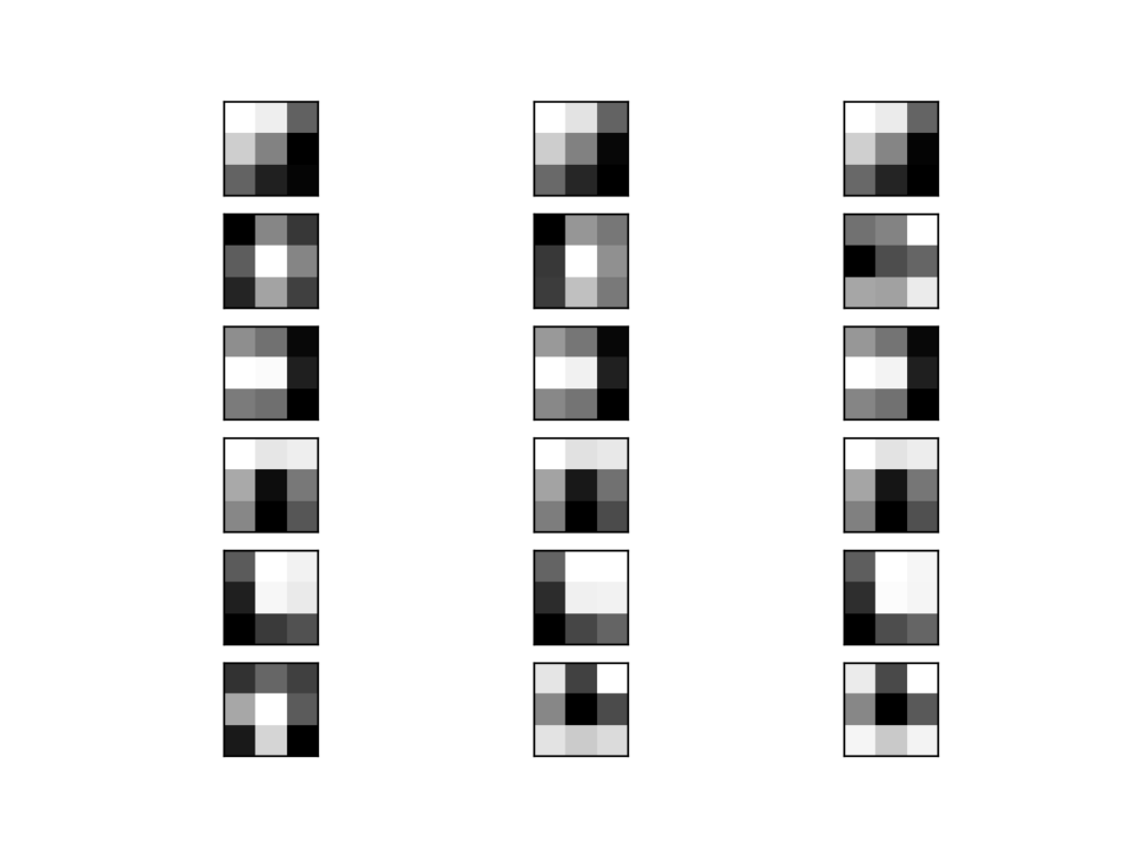
Plot of the First 6 Filters From VGG16 With One Subplot per Channel
Although we have a visualization, we only see the first six of the 64 filters in the first convolutional layer. Visualizing all 64 filters in one image is feasible.
Sadly, this does not scale; if we wish to start looking at filters in the second convolutional layer, we can see that again we have 64 filters, but each has 64 channels to match the input feature maps. To see all 64 channels in a row for all 64 filters would require (64×64) 4,096 subplots in which it may be challenging to see any detail.
How to Visualize Feature Maps
The activation maps, called feature maps, capture the result of applying the filters to input, such as the input image or another feature map.
The idea of visualizing a feature map for a specific input image would be to understand what features of the input are detected or preserved in the feature maps. The expectation would be that the feature maps close to the input detect small or fine-grained detail, whereas feature maps close to the output of the model capture more general features.
In order to explore the visualization of feature maps, we need input for the VGG16 model that can be used to create activations. We will use a simple photograph of a bird. Specifically, a Robin, taken by Chris Heald and released under a permissive license.
Download the photograph and place it in your current working directory with the filename ‘bird.jpg‘.
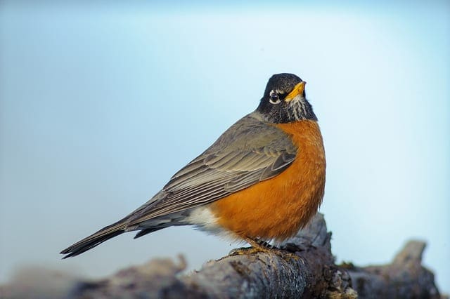
Robin, by Chris Heald
Next, we need a clearer idea of the shape of the feature maps output by each of the convolutional layers and the layer index number so that we can retrieve the appropriate layer output.
The example below will enumerate all layers in the model and print the output size or feature map size for each convolutional layer as well as the layer index in the model.
|
1 2 3 4 5 6 7 8 9 10 11 12 13 |
# summarize feature map size for each conv layer from keras.applications.vgg16 import VGG16 from matplotlib import pyplot # load the model model = VGG16() # summarize feature map shapes for i in range(len(model.layers)): layer = model.layers[i] # check for convolutional layer if 'conv' not in layer.name: continue # summarize output shape print(i, layer.name, layer.output.shape) |
Running the example, we see the same output shapes as we saw in the model summary, but in this case only for the convolutional layers.
|
1 2 3 4 5 6 7 8 9 10 11 12 13 |
1 block1_conv1 (?, 224, 224, 64) 2 block1_conv2 (?, 224, 224, 64) 4 block2_conv1 (?, 112, 112, 128) 5 block2_conv2 (?, 112, 112, 128) 7 block3_conv1 (?, 56, 56, 256) 8 block3_conv2 (?, 56, 56, 256) 9 block3_conv3 (?, 56, 56, 256) 11 block4_conv1 (?, 28, 28, 512) 12 block4_conv2 (?, 28, 28, 512) 13 block4_conv3 (?, 28, 28, 512) 15 block5_conv1 (?, 14, 14, 512) 16 block5_conv2 (?, 14, 14, 512) 17 block5_conv3 (?, 14, 14, 512) |
We can use this information and design a new model that is a subset of the layers in the full VGG16 model. The model would have the same input layer as the original model, but the output would be the output of a given convolutional layer, which we know would be the activation of the layer or the feature map.
For example, after loading the VGG model, we can define a new model that outputs a feature map from the first convolutional layer (index 1) as follows.
|
1 2 |
# redefine model to output right after the first hidden layer model = Model(inputs=model.inputs, outputs=model.layers[1].output) |
Making a prediction with this model will give the feature map for the first convolutional layer for a given provided input image. Let’s implement this.
After defining the model, we need to load the bird image with the size expected by the model, in this case, 224×224.
|
1 2 |
# load the image with the required shape img = load_img('bird.jpg', target_size=(224, 224)) |
Next, the image PIL object needs to be converted to a NumPy array of pixel data and expanded from a 3D array to a 4D array with the dimensions of [samples, rows, cols, channels], where we only have one sample.
|
1 2 3 4 |
# convert the image to an array img = img_to_array(img) # expand dimensions so that it represents a single 'sample' img = expand_dims(img, axis=0) |
The pixel values then need to be scaled appropriately for the VGG model.
|
1 2 |
# prepare the image (e.g. scale pixel values for the vgg) img = preprocess_input(img) |
We are now ready to get the feature map. We can do this easy by calling the model.predict() function and passing in the prepared single image.
|
1 2 |
# get feature map for first hidden layer feature_maps = model.predict(img) |
We know the result will be a feature map with 224x224x64. We can plot all 64 two-dimensional images as an 8×8 square of images.
|
1 2 3 4 5 6 7 8 9 10 11 12 13 14 |
# plot all 64 maps in an 8x8 squares square = 8 ix = 1 for _ in range(square): for _ in range(square): # specify subplot and turn of axis ax = pyplot.subplot(square, square, ix) ax.set_xticks([]) ax.set_yticks([]) # plot filter channel in grayscale pyplot.imshow(feature_maps[0, :, :, ix-1], cmap='gray') ix += 1 # show the figure pyplot.show() |
Tying all of this together, the complete code example of visualizing the feature map for the first convolutional layer in the VGG16 model for a bird input image is listed below.
|
1 2 3 4 5 6 7 8 9 10 11 12 13 14 15 16 17 18 19 20 21 22 23 24 25 26 27 28 29 30 31 32 33 34 35 36 37 |
# plot feature map of first conv layer for given image from keras.applications.vgg16 import VGG16 from keras.applications.vgg16 import preprocess_input from keras.preprocessing.image import load_img from keras.preprocessing.image import img_to_array from keras.models import Model from matplotlib import pyplot from numpy import expand_dims # load the model model = VGG16() # redefine model to output right after the first hidden layer model = Model(inputs=model.inputs, outputs=model.layers[1].output) model.summary() # load the image with the required shape img = load_img('bird.jpg', target_size=(224, 224)) # convert the image to an array img = img_to_array(img) # expand dimensions so that it represents a single 'sample' img = expand_dims(img, axis=0) # prepare the image (e.g. scale pixel values for the vgg) img = preprocess_input(img) # get feature map for first hidden layer feature_maps = model.predict(img) # plot all 64 maps in an 8x8 squares square = 8 ix = 1 for _ in range(square): for _ in range(square): # specify subplot and turn of axis ax = pyplot.subplot(square, square, ix) ax.set_xticks([]) ax.set_yticks([]) # plot filter channel in grayscale pyplot.imshow(feature_maps[0, :, :, ix-1], cmap='gray') ix += 1 # show the figure pyplot.show() |
Running the example first summarizes the new, smaller model that takes an image and outputs a feature map.
Remember: this model is much smaller than the VGG16 model, but still uses the same weights (filters) in the first convolutional layer as the VGG16 model.
|
1 2 3 4 5 6 7 8 9 10 11 |
_________________________________________________________________ Layer (type) Output Shape Param # ================================================================= input_1 (InputLayer) (None, 224, 224, 3) 0 _________________________________________________________________ block1_conv1 (Conv2D) (None, 224, 224, 64) 1792 ================================================================= Total params: 1,792 Trainable params: 1,792 Non-trainable params: 0 _________________________________________________________________ |
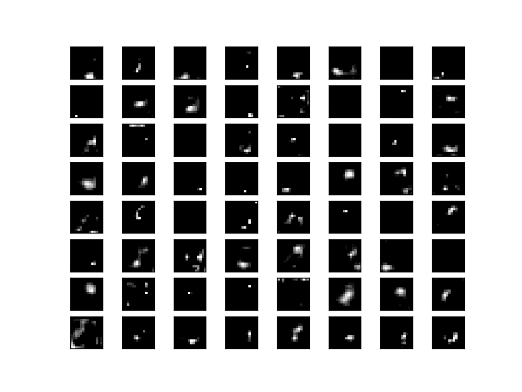
Next, a figure is created that shows all 64 feature maps as subplots.
We can see that the result of applying the filters in the first convolutional layer is a lot of versions of the bird image with different features highlighted.
For example, some highlight lines, other focus on the background or the foreground.
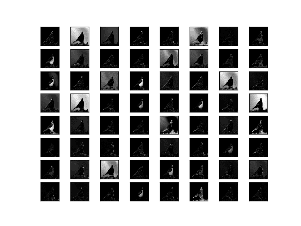
Visualization of the Feature Maps Extracted From the First Convolutional Layer in the VGG16 Model
This is an interesting result and generally matches our expectation. We could update the example to plot the feature maps from the output of other specific convolutional layers.
Another approach would be to collect feature maps output from each block of the model in a single pass, then create an image of each.
There are five main blocks in the image (e.g. block1, block2, etc.) that end in a pooling layer. The layer indexes of the last convolutional layer in each block are [2, 5, 9, 13, 17].
We can define a new model that has multiple outputs, one feature map output for each of the last convolutional layer in each block; for example:
|
1 2 3 4 5 |
# redefine model to output right after the first hidden layer ixs = [2, 5, 9, 13, 17] outputs = [model.layers[i+1].output for i in ixs] model = Model(inputs=model.inputs, outputs=outputs) model.summary() |
Making a prediction with this new model will result in a list of feature maps.
We know that the number of feature maps (e.g. depth or number of channels) in deeper layers is much more than 64, such as 256 or 512. Nevertheless, we can cap the number of feature maps visualized at 64 for consistency.
|
1 2 3 4 5 6 7 8 9 10 11 12 13 14 15 16 |
# plot the output from each block square = 8 for fmap in feature_maps: # plot all 64 maps in an 8x8 squares ix = 1 for _ in range(square): for _ in range(square): # specify subplot and turn of axis ax = pyplot.subplot(square, square, ix) ax.set_xticks([]) ax.set_yticks([]) # plot filter channel in grayscale pyplot.imshow(fmap[0, :, :, ix-1], cmap='gray') ix += 1 # show the figure pyplot.show() |
Tying these changes together, we can now create five separate plots for each of the five blocks in the VGG16 model for our bird photograph. The complete listing is provided below.
|
1 2 3 4 5 6 7 8 9 10 11 12 13 14 15 16 17 18 19 20 21 22 23 24 25 26 27 28 29 30 31 32 33 34 35 36 37 38 39 40 |
# visualize feature maps output from each block in the vgg model from keras.applications.vgg16 import VGG16 from keras.applications.vgg16 import preprocess_input from keras.preprocessing.image import load_img from keras.preprocessing.image import img_to_array from keras.models import Model from matplotlib import pyplot from numpy import expand_dims # load the model model = VGG16() # redefine model to output right after the first hidden layer ixs = [2, 5, 9, 13, 17] outputs = [model.layers[i].output for i in ixs] model = Model(inputs=model.inputs, outputs=outputs) # load the image with the required shape img = load_img('bird.jpg', target_size=(224, 224)) # convert the image to an array img = img_to_array(img) # expand dimensions so that it represents a single 'sample' img = expand_dims(img, axis=0) # prepare the image (e.g. scale pixel values for the vgg) img = preprocess_input(img) # get feature map for first hidden layer feature_maps = model.predict(img) # plot the output from each block square = 8 for fmap in feature_maps: # plot all 64 maps in an 8x8 squares ix = 1 for _ in range(square): for _ in range(square): # specify subplot and turn of axis ax = pyplot.subplot(square, square, ix) ax.set_xticks([]) ax.set_yticks([]) # plot filter channel in grayscale pyplot.imshow(fmap[0, :, :, ix-1], cmap='gray') ix += 1 # show the figure pyplot.show() |
Running the example results in five plots showing the feature maps from the five main blocks of the VGG16 model.
We can see that the feature maps closer to the input of the model capture a lot of fine detail in the image and that as we progress deeper into the model, the feature maps show less and less detail.
This pattern was to be expected, as the model abstracts the features from the image into more general concepts that can be used to make a classification. Although it is not clear from the final image that the model saw a bird, we generally lose the ability to interpret these deeper feature maps.
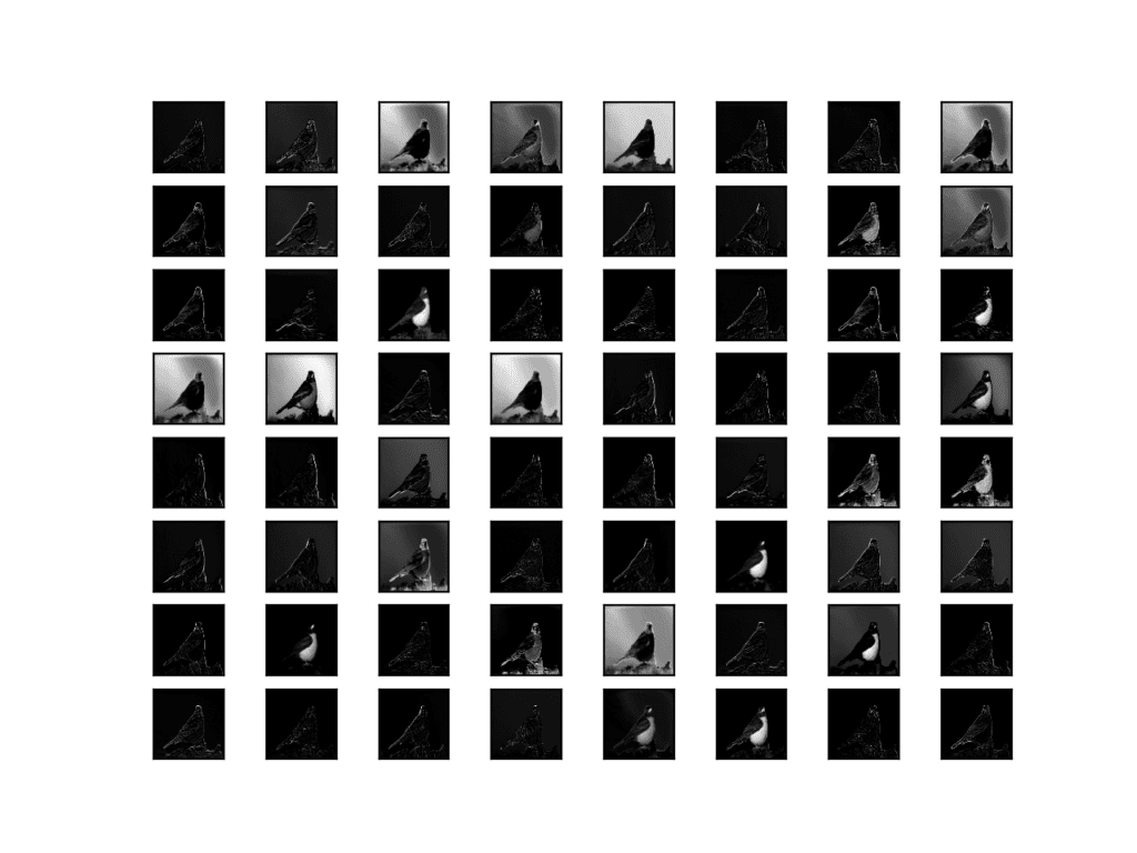
Visualization of the Feature Maps Extracted From Block 1 in the VGG16 Model
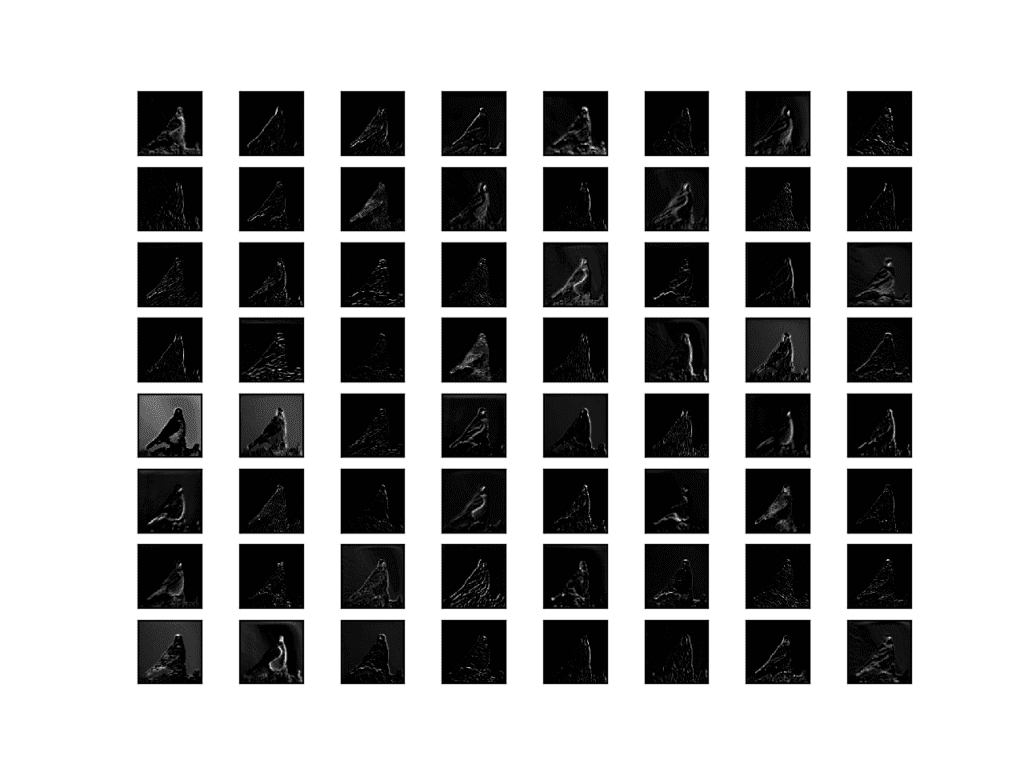
Visualization of the Feature Maps Extracted From Block 2 in the VGG16 Model
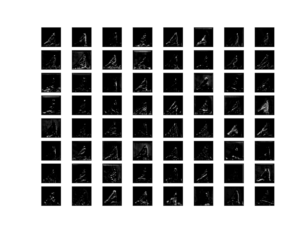
Visualization of the Feature Maps Extracted From Block 3 in the VGG16 Model
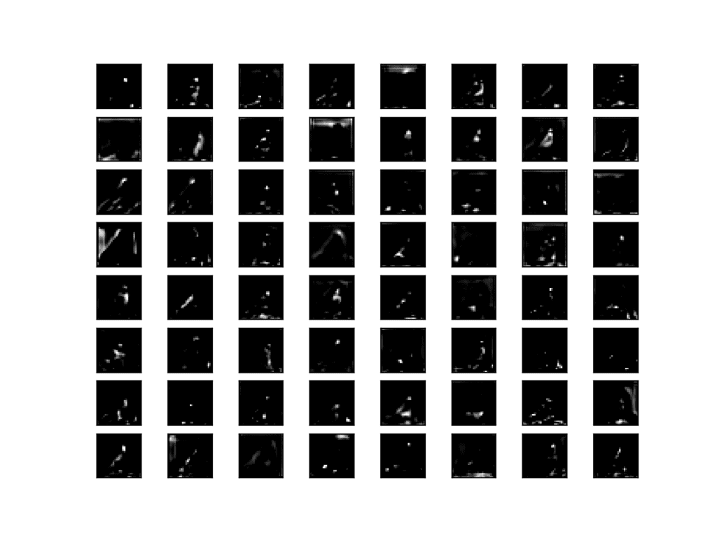
Visualization of the Feature Maps Extracted From Block 4 in the VGG16 Model
Visualization of the Feature Maps Extracted From Block 5 in the VGG16 Model
Further Reading
This section provides more resources on the topic if you are looking to go deeper.
Books
- Chapter 9: Convolutional Networks, Deep Learning, 2016.
- Chapter 5: Deep Learning for Computer Vision, Deep Learning with Python, 2017.
API
Articles
- Lecture 12 | Visualizing and Understanding, CS231n: Convolutional Neural Networks for Visual Recognition, (slides) 2017.
- Visualizing what ConvNets learn, CS231n: Convolutional Neural Networks for Visual Recognition.
- How convolutional neural networks see the world, 2016.
Summary
In this tutorial, you discovered how to develop simple visualizations for filters and feature maps in a convolutional neural network.
Specifically, you learned:
- How to develop a visualization for specific filters in a convolutional neural network.
- How to develop a visualization for specific feature maps in a convolutional neural network.
- How to systematically visualize feature maps for each block in a deep convolutional neural network.
Do you have any questions?
Ask your questions in the comments below and I will do my best to answer.
Develop Deep Learning Models for Vision Today!

Develop Your Own Vision Models in Minutes
...with just a few lines of python code
Discover how in my new Ebook:
Deep Learning for Computer Vision
It provides self-study tutorials on topics like:
classification, object detection (yolo and rcnn), face recognition (vggface and facenet), data preparation and much more...
Finally Bring Deep Learning to your Vision Projects
Skip the Academics. Just Results.


")
")

Thanks a lot, sir!! It helps my thesis manuscript in finding feature maps in each layer in my model. By the way, I have a question sir about how to display in values (not an image) in each filters and biases in every convolutional layer in my CNN model?
I’m happy to hear that.
You could print the arrays and inspect the values.
Okay sir thank you 🙂
Sir can I make a request, I would like to display every feature maps in every convolutional layer in my model and I have a problem of my code in accessing all feature maps in every layer. Any suggestion sir? I hope your response sir and thank you.
Excellent explanation sir
index = [0, 1, 6, 9, 14, 17]
outputs = [self.model.layers[i].output for i in index]
self.model = Model(inputs=self.model.inputs, outputs=outputs)
featureMaps = self.model.predict(self.testImage)
print((np.shape(featureMaps[0][0])))
print(“FeatureMapsLen: “+str(np.shape(featureMaps[0]))[2])
numOfFeaturemaps = (np.shape(featureMaps[0][0]))[2]
print(“numOfFeatureMaps: “+str(numOfFeaturemaps)
fig=plt.figure(figsize=(16,16))
subplotNum=int(np.ceil(np.sqrt(numOfFeaturemaps)))
for i in range(int(numOfFeaturemaps)):
idx = fig.add_subplot(subplotNum, subplotNum, i+1)
idx.imshow(featureMaps[0, :, :, i], cmap=’viridis’) #I’m have been stack here for long sir jason!!
plt.xticks(np.array([]))
plt.yticks(np.array([]))
plt.tight_layout()
plt.savefig(“featureMaps/featuremaps@Layer{}”.format(self.layerNum) + ‘.png’)
outputImg = QtGui.QPixmap(“featureMaps/featuremaps@Layer{}”.format(self.layerNum) + ‘.png’)
self.userInterface.labelImageContainer.setScaledContents(False)#Fixed display
self.userInterface.labelImageContainer.setPixmap(outputImg)
This is a common question that I answer here:
https://machinelearningmastery.com/faq/single-faq/can-you-read-review-or-debug-my-code
LiME is known to “explain” the results of a classification problem. Can we use the filters that you have explained in order to explain the results of a segmentation problem?
Perhaps. I have not seen any work on the topic.
Perhaps try searching on scholar.google.com.
great explanation. The best part is step by step explanation with code. Really helpful 🙂
Thanks.
For no apparent reason, I have my Keras via TensorFlow so I have to modify, for instance, this line of code:
“from keras.applications.vgg16 import VGG16”
to
“from tensordlow.keras.applications.vgg16 import VGG16”
and when I loaded it for the first time it showed it was downloading from Github but then it is now training! Is this normal?
Thanks!
It is downloaded the first time. That is normal.
Right! But I had a difficulty to download it and after 33Mb I got disconnection from remote server error so I opened vgg16.py located in my tensorflow/python/keras/applications, got the link, downloaded manually and change the default from ‘imagenet’ to the path that the manually downloaded file was located (I transferred it to ‘applications’ folder but still asked me the whole path and not only the filename: ‘vgg16_weights_tf_dim_ordering_tf_kernels.h5’) so it worked out for me. Would you mind if you kindly tell me why it asked the whole path? It should recognized its current path as it’s running in it.
I don’t know why it asked for the full path, sorry.
Hi Hamed, I’ll just note that TensorFlow gets updated so rapidly that,what was true yesterday about a specific niche detail about the TensorFlow implementation, might not be True the next day. Sometimes the only available documentation is the source code for your specific version. You can read the source code if it’s worth it, or ask for help on stackoverflow.com or github.com/tensorflow but it is often not worth it as updating the TF version will fix the problem at hand.
Agreed! Thanks for sharing.
Thanks for the lesson!!
I would love to see a detailed description of how to create class activation maps.
I’ve been using some of the code from your books to train a CNN to recognize tears of the anterior crucial efforts ligament. I’d love to see just what parts of the image my model is using to make its decisions.
Anterior cruciate ligament, that is.
Nice, sounds like xray scans or similar.
Great suggestion, thanks.
Well done on your application Mike!
Thanks, that’s very kind of you .
Hello Jason,
Thanks for your code..It really helpful.
I have a query here.
1. We are using single image in this model instead is it possible to use batch of images to visualise them in the model ?
2. I am a newbie. Don’t mind me for a silly question here please. Is it possible to view outputs at fully connected layers like Conv layers we did here?
3. Is there any limit on number of neurons used in dense layers?
You would process one image at a time, if you are only looking at activation maps.
You can review activations of any layer, but Dense layers will not form images, it will be noise.
The only limit is the mount of RAM you have.
How to save feature maps as png or pdf
If you plot them, you can save the plots to file.
In matplotlib there is a savefig() function:
https://matplotlib.org/3.1.0/api/_as_gen/matplotlib.pyplot.savefig.html
Hey love the detailed description of what you have done!
I am trying to replicate the same but then for a pytorch model.
So the models look different and I cannot use the same functions to create the feature map.
Any change you did the same for a pytorch model or maybe give me some advise on how to?
Currently I am complete stuck on how to do this.
Sorry, I don’t have any pytorch examples, I cannot give you good off the cuff advice.
Hi Jason,
Hwo to fix the following issue ?
NameError: name ‘Model’ is not defined
after execute
model = Model(inputs=model.inputs, outputs=model.layers[1].output)
Thanks.
The error suggests that you have not imported the Model class.
I got it.
Thank you very much!
hi i’ve the same error and i am new coder. What should I do to fix this error
Perhaps some of these tips will help:
https://machinelearningmastery.com/faq/single-faq/why-does-the-code-in-the-tutorial-not-work-for-me
Hi Jason, another nice posting from you.
I have a stupid question: I understand that layer closer to the input will learn local feature while layer close to the output will learn global feature. For example: I have an image of face and I feed this image to my VGG16 network. When I visualize the filter, I expect that the earlier will draw “eyebrow”, “nose” and last layer will describe “face”, but I am totally wrong.
So, I thought local feature = “eyebrow”, “nose”, but activation maps of first filter describe “face” (global feature).
Can you explain to me about this matter? Thanks.
It really depends on the specific model.
Another question, how can a model infer the object to be, for example, cat or dog if the last convolution layer is unclear/less detail even for human? Thanks.
The model has a classifier layer at the output to interpret the high order features.
Hi Jason
I am using ResNet50 instead of VGG16 but while executing the following code I get an error:
ValueError: not enough values to unpack (expected 2, got 0)
from keras.applications.resnet50 import ResNet50
from matplotlib import pyplot
model = ResNet50()
for layer in model.layers:
if ‘conv’ not in layer.name:
continue
# get filter weights
filters, biases = layer.get_weights()
print(layer.name, filters.shape)
The error is related to the line: filters, biases = layer.get_weights()
The resnet architecture is more complex, you will have to debug this change.
Thanks, Jason. Figured it out eventually.
I’m happy to hear that.
would you share your code please?
Please, can you share how you solve it. Thank you.
You are awesome.You made the concepts clear.THANK YOU SO MUCH
Thanks, I’m glad it helped!
Thank you for your great articles. I often read your blog from ‘random’ google searches.
You are awesome!
Thanks Simone!
One of the most difficult and hot topics explained in a very simple and informative way. I really appreciate the way you explained. One of my favorite blogs ever. Thanks, Jason!
Thanks, I’m glad it helped!
Is it possible to do that when working on time series? I was looking at these examples (https://machinelearningmastery.com/how-to-develop-rnn-models-for-human-activity-recognition-time-series-classification/) and I would like to try to explain something about what the model is understanding. I extrapolated the output of the Conv layers and I have visualized it for each different class but I would like to know what are your thoughts about that.
It may be possible, I have not tried.
It is one of the best tutorial for beginner ,,thank you sir
sir I have one doubt in cov2d function “filter” one of the parameter ,what value it will take as the matrix value which is matrix multiplication with the convolution image (I seen this in vgg16() function) is this take labelled matrix value (if it is in supervised)
Thanks, I’m glad it helped.
The weights or filters will take on weights learned during the training process.
Thank you sir , and i also wants to know how the weights are updated for each layer, is there any method to update it
note: i am trying to understand the architecture model https://arxiv.org/pdf/1511.00561 segnet and also each and every functions , thank you sir
Weights are updated via backpropagation.
Sorry I am not familiar with that paper, perhaps contact the author.
Why is there a need to make a new model so as to see the output from each layer? Instead can we not directly use
model = VGG16()
model.predict(img)
for i in enumerate(model.layers):
model.layers[i].output
so as to visualize the output per layer of the VGG model directly, without having to create a new model?
It is not really a new model, just a view on the existing model.
Thank you for your great effort sir!!
CNN is also used for text classification. So can we use same technique to visualize feature map and filter for text classification(not for plot image).For example which words or features that the model used to discriminate class.Thank in advance
I don’t see why not, it’s a great idea!
Let me know how you go.
Hello Jason Brownlee!
As usual a great thanks for your work, a golden mine of clear information!
I am currently using GradCam, to see the most activating pixels convolutions after convolutions. But for example, if we take just a simple ConvNet with one conv layer, for a task such (Fashion) MNIST dataset, which would already give decent results.
With GradCamm, Saliency Maps and other conv visualisation techniques, we could only “see” one image at a time. But how could we “do stastistics” on a whole dataset. For example, to see how a “general digit 1” is seen by the network.
I have searched for articles/papers, but couldn’t find anaything. I know visualisation techniques are quite recents, but they still are only able to process one image at a time.
Would you have some interesting papers about it?
Thanks again for your kindness and precious work!
What types of statistics do you want to do on the whole dataset exactly?
What question would you be answering?
There are many good papers on the topic, perhaps search on scholar.google.com
Yes I searched on Google/Google Scholar to see what had already been done, but perharps I did not use the good keywords…
For example, I searched for (Grad)CAM/Saliency Maps statistics. I don’t have a clear goal for my searhc, but as I said I am interested in any method that could transform the “image-per-image” explanation to a technique that allows to perform statistics.
For example I tried to just compute the mean of all GradCam for all images of a given predicted class with MNIST (for a fixed conv layer), and of course I could see a “global” form of the digit. But that is just a really simple thing to do..
It would be really kind of you if you could give a paper or better keywords to searched for on Google Scholar.
Thanks again for your time and patience!
Perhaps skim through the top CNN viz papers, if nothing pops up, perhaps you have to develop something from scratch.
Perhaps sketch what you want with some numpy examples to confirm the question you’re asking about the data/model is tractable.
No breakpoint-continue? If the downloading of the model is interrupted, then it will do downloading from the very beginning. Is it possible to download only the remaining? will save a lot of time. Thanks.
Download?
Do you mean train? I so, you can use checkpoints:
https://machinelearningmastery.com/check-point-deep-learning-models-keras/
Sir can you guide me how to lexicographically sort the feature maps. I need it copy move forgery detection.
There is no lexicon (words) to sort. What do you mean exactly?
Sir,
This is a wonderful explanation.
I am doing this with a custom dataset with my own model, which is a slight variation of resnet.
What do I do with the part where pixel values are scaled with img = preprocess_input(img)
I cannot import keras.application.Resnet50 as dataset is custom made.
Thanks.
You must prepare pixels in the way that the resnet expects. You can do this with a helper function in Keras or manually.
Hi Jason Thanks for your awesome Tutorial
I have a question :
I want to save my extracted features after fully concocted layer before softamx how can I do this?
let’s explain more my problem in easy way I want to get an image then instead of using pixels as features I want to extract them from CNN ,after convolution layer before softmax,on the other hand I want to change classification method instead of using softamax for example using KNN or SVM,do you have any idea how can I do this?
I want to this something like this paper
https://www.sciencedirect.com/science/article/abs/pii/S0167865519300868
Yes, I give an example for face recognition here:
https://machinelearningmastery.com/how-to-develop-a-face-recognition-system-using-facenet-in-keras-and-an-svm-classifier/
Do you ever feel like a hero, I hope you do, because for me you are undoubtedly one of them, save my week.
Thanks.
Thanks.
Yes, you can remove the output layer and save the feature vector directly. I give an example here:
https://machinelearningmastery.com/how-to-use-transfer-learning-when-developing-convolutional-neural-network-models/
Dear Brownlee,
You clarify hard problems step by step and turn them into an easy to understand issue. Thank you very much for your effort. I also appreciate that you share your knowledge and save a lot of time of us. I am sure that, anyone who interested in ml, visit your website at least once in a life. So, please keep on helping us.
My question is that I want to apply this visualization method to resnet model trained with timeseries instead of images.
Do you think, is it reasonable to apply for time series?
Thanks!
No, I don’t think it would be appropriate for time series. The visualization is suited for images.
I am a bit confused about whether we can use this method for timeseries or not
You replied Rango’s question as
“I don’t see why not, it’s a great idea!
Let me know how you go.”
Rango’s question:
Thank you for your great effort sir!!
CNN is also used for text classification. So can we use same technique to visualize feature map and filter for text classification(not for plot image).For example which words or features that the model used to discriminate class.Thank in advance
I don’t think so, but I don’t want to rule anything out.
Oh , I got it. If it won’t be so many questions, what are your concerns, why do you think it is not that proper?
Images are a visual medium, it makes sense to visualize how the models “sees” the inputs.
Thank you
You’re welcome.
Dear Sir,
Thanks for the very clear and good explanation about visualising cnn filters and feature maps.
I am very confused on one part. My question is that each block output of CNN layers are of different down sampled output sizes.
For Example:
block1_conv2 (?, 224, 224, 64) input image shape
block2_conv1 (?, 112, 112, 128) down sampled output size.
and soon…..
But when we are visualising the intermediate layers output we are getting the output image with the shape of (224,224,3).
1.Why we are not getting the downsampled output image with shape of (112, 112, 3)?
2. Is it possible to visualize the actual downsampled output images from all intermediate layers?
please kindly guide me and also help me with some code snippets.
You’re welcome.
We do have a visualization at each block with different sizes.
This can be seen in the output images and when we print the shape of the output of each block.
the example model is in format, is it possible for the code read .npy format?
example is .h5
You can save the model anyway you wish.
The built-in library uses h5 format.
I do not have an example of using custom code to save the model weights.
Sorry, I don’t understand. Perhaps you can elaborate?
Dear Sir
The shape of the output at each block was as expected. I have few doubts
1. In a sequential cnn operation the input size for example (224,224) will be preserved in each blocks?
2. In this article why we are not following the sequential cnn operation flow of visualization in each blocks?
3. Every time for visualizing the intermediate block layers why we are making the input images to the size of (224,224) ? For example vggnet expects the input shape to be 224,224 at the first conv block layer and after that in the next successive blocks what will be input image and its size, Whether we have to give the downsampled image(for example: (112,112) or (56,56) or (28,28) and soon) as the input to the successive conv blocks or how?
getting confused here.
please kindly guide me.
No. Each layer will change the shape.
You can learn more about the effect of convolutional layers here:
https://machinelearningmastery.com/convolutional-layers-for-deep-learning-neural-networks/
You can learn more about the effect of pooling layers here:
https://machinelearningmastery.com/pooling-layers-for-convolutional-neural-networks/
Sir,
is the first convolutional layer output feature map is the input to next convolutional layer and what is the input size for second and other convolutional layers.
Yes, models a sequence of layers connected linearly.
Dear sir
For visualizing purpose from any of the intermediate block layers why we are making the input images to the size of (224,224)? Why we are not giving the previous layer output as the input to the next layer?
please kindly guide me.
thanking you
Perhaps review the output of the model summary to see the order of layers and their output shapes.
Within the text it is said: “For example, we can design and understand small filters, such as line detectors.” Do you have any tutorials on your website about designing special-purpose filters and their applications? I appreciate if you share the link.
Yes, here’s an example of a line filter:
https://machinelearningmastery.com/convolutional-layers-for-deep-learning-neural-networks/
thanks a lot
You’re welcome.
Hi Jason,
Great article,
I am using a 3d kernel of size 3x3x3 in my conv layer and would like to get similar weight visualization plots.
Since plotting in 3d is not possible i tried to split the kernels into 3 3×3 for plotting.
Is this approach correct?
The conv layer consists of 5 layers #model.add(layers.Conv3D(5, (3, 3, 3), padding=’same’))
Please find below the code I used to plot the weights adapted from your code and do let me know if this approach is correct or is there any better method..
from keras.models import load_model
mymodel = load_model(‘model.hdf5′)
from matplotlib import pyplot as plt
# load the model
# retrieve weights from the 1st conv layer layer
filters, biases = mymodel.layers[0].get_weights()
# normalize filter values to 0-1 so we can visualize them
f_min, f_max = filters.min(), filters.max()
filters = (filters – f_min) / (f_max – f_min)
#shape of filters (3, 3, 3, 1, 5)
n_filters, ix = 5, 1
for i in range(n_filters):
# get the filter
f = filters[:,:, :, :, i]
f = f[:,:,:,0]
# kernel shape 3x3x3 but to plot it converting into 3 3×3 filters
for j in range(3):
# specify subplot and turn of axis
ax = plt.subplot(n_filters, 3, ix)
ax.set_xticks([])
ax.set_yticks([])
# plot filter channel in grayscale
plt.imshow(f[:, :, j], cmap=’gray’)
ix += 1
# show the figure
plt.show()
Looking forward to your reply
This is a common question that I answer here:
https://machinelearningmastery.com/faq/single-faq/can-you-read-review-or-debug-my-code
I am only asking for your suggestion and not to review my code, just want to know whether the method that I used is correct or not or any further suggestions..
Sorry, I don’t have examples of working with 3d conv nets. In order to figure out if what you have done is reasonable I need to read/review your new code – which I don’t have the capacity to do.
Perhaps try posting on stackoverflow?
Thank you! This is really helpful.
You’re welcome!
Dear Sir,
Thanks for the great article.
I do not understand why the features of the initial CNN layer are more prominent than the higher layer? For object classification, features of the final layer should be more clear for identification.
Please clarify.
The data flowing through the model is most like the original data towards the input end of the model before any pooling or processing has been performed.
Hello
How can I fix this error in this line of code?
inter_output_model = tf.keras.Model (model.input, model.get_layer (index = 1) .output)
AttributeError: ‘tuple’ object has no attribute ‘layer’
And in this error in this line
from matplotlib import pyplot as plt
import numpy as np
# plot all 64 maps in an 8×8 squares
square = 8
ix = 1
for _ in range (square):
for _ in range (square):
# specify subplot and turn of axis
ax = pyplot.subplot (square, square, ix)
ax.set_xticks ([])
ax.set_yticks ([])
# full filter channel in grayscale
pyplot.imshow (feature_maps [0,:,,:, ix-1], cmap = ‘gray’)
ix + = 1
# show the figure
pyplot.show ()
IndexError: too many indices for array
Thanks for the tutorial
This is a common question that I answer here:
https://machinelearningmastery.com/faq/single-faq/can-you-read-review-or-debug-my-code
Holy moly! I’ve got everything I was looking for in a single article! Great work! Thanks for drafting such a piece.
I’m happy to hear that!
Great article, Jason!
One quick question: if I want to further cluster the birds into subtypes (of birds) with unsupervised learning, what would you suggest? I am thinking of using the feature maps as input for unsupervised clustering, then which layers would make sense to you?
Thanks so much!
Interesting.
Perhaps a clustering algorithm?
Thank you for the great article Jason!
I was wondering whether you have any plans on writing an article on “Visualizing and Understanding Convolutional Networks” by Zeiler et al. or a summary of work following that?
This would be really helpful.
Thanks for the suggestion.
How identify no. Of nodes for dense layer in cnn image classification.
Realy wana formula to specify it .
Good question, see this:
https://machinelearningmastery.com/faq/single-faq/how-many-layers-and-nodes-do-i-need-in-my-neural-network
Great and simple Jason!
I would like to know if it is possible to visualize the feature from fc1 and f2 despite the dimensionality reduction? If yes, can you please guide in the right direction?
Not really as there are no feature maps in dense layers.
That strange! According to limited understanding of fully connected layers is that they consist of patches of features of the object of a particular class which then pass to a prediction layer to make predictions. Is it the wrong interpretation?
Furthermore, I just went through the link (https://de.mathworks.com/help/deeplearning/ug/visualize-features-of-a-convolutional-neural-network.html), which shows how to Visualize the features of Fully Connected Layer (FC-layers) using deepDreamImage in Matlab. I just wanted to do the same in Keras.
Perhaps some of the references in the “further reading” section of the tutorial will help as a starting point.
Thanks for really helpful article. I read so many your articles. And I have one question for here.
‘How can I transfer the functions of a deep neural network?’ thesis or transfer learning
The first layer comes with general features like lines, edges, and stains, and the last layer has certain features. However, you need to pass the image to this article or VGG16. The first layer is the input image area.
Am I misunderstanding. Can I ask for an explanation?
According to your article, the first layer shows a detailed image similar to the input image, and the last layer shows a less detailed blob-like image. While I did the test with VGG16, it was similar to your result.
But, the thesis “How transferable are features in deep neural networks?” and articles explaining the reason for Transfer Learning said that less detailed images such as lines, edges, and blobs appears in the first layer, and specific features are showed in the last layer.
So, can you explain why the reason of differences between yours and others?
Perhaps ask the author of the document you are referencing?
You can see my code directly and the results.
i am trying to visualize layers using mobilenet(keras). The shape of feature map after model.predict is (1,225,225,3). while plotiing i am getting the following error. can anyone help me with this.
IndexError Traceback (most recent call last)
in ()
11 ax.set_yticks([])
12 # plot filter channel in grayscale
—> 13 pyplot.imshow(feature_maps[0, :, :, ix-1], cmap=’gray’)
14 ix += 1
15 # show the figure
IndexError: index 3 is out of bounds for axis 3 with size 3
Sorry, I’m not sure of the cause of the fault.
Perhaps try posting your code to stackoverflow?
Hi,
I was trying to follow your code and apply it to Xception network. But when I tried to retrieve the filters and biases, I got –
—————————————————————————
ValueError Traceback (most recent call last)
1 # retrieve weights from the second hidden layer
—-> 2 filters, biases = model.layers[1].get_weights()
ValueError: not enough values to unpack (expected 2, got 1)
Please help me.
Thanks
AM
Sorry to hear that, the cause of the fault is not obvious to me, you may need to debug your changes.
Hi Jason,
Thank you for your answer. I tried to debug it. I can access each layer filter but for the problem is happening when I try to print all filters shape. I believe, if condition statement will be different for Xcepion. But I am not sure what it will be.
model = Xception()
for layer in model.layers:
# check for convolutional layer
if ‘conv’ not in layer.name:
continue
# get filter weights
filters, biases = layer.get_weights()
print(layer.name, filters.shape)
Error message : ValueError: not enough values to unpack (expected 2, got 1)
Could you please have a look?
Thank you.
Kind regards,
Alakananda
Sorry, I don’t have the capacity to debug your code example. Perhaps these tips will help:
https://machinelearningmastery.com/faq/single-faq/can-you-read-review-or-debug-my-code
please ,how to save the ouput feature maps images in folder
Perhaps save the images directly, see this:
https://machinelearningmastery.com/how-to-load-and-manipulate-images-for-deep-learning-in-python-with-pil-pillow/
ok thanks for your reply , but i want the code to save the output feature maps I get from this article in new folder not for simple image .
Yes, the code in the linked tutorials hows you how to save an image.
Thanks a lot for this great article, I am teaching image recognition and data science, and really I learned a lot from thanks again.
I would like to ask you two questions regarding visualizing feature maps from CNN:
1- how we can benefits from a visualization for improving model accuracy by either change architecture of CNN or even update filers ( more training)
2- before ready this article, I expected the output from the first layer recognizes low-level edges, then the next layer to recognizes higher-level edges, till the end recognizes the whole object but surprised by the reversed order. Can you confirm my understanding
You’re welcome.
You’re understanding is correct, it is just operating at the scale of the whole image.
Hi Jason,
Wonderful article.
Can you please let me know how I can get the list of fired neurons in a CNN model when an image is fed to it for a prediction.
For example a CNN model predicts fruit name if an image of a fruit is fed to it. If I feed an image of an apple, can I get the data of hidden layers like:
{ {Layer-1}, {N1, N20, N24, N55, N100..N150} },
{ {Layer-2}, {N21, N50, N75..N90} }
here the N represents the neuron number of a given layer that fired to make the prediction. The gap between the neuron numbers indicates the neurons that did not fire.
Your help is much appreciated.
The above tutorials is exactly what you describe.
Hi Jason,
I guess I phrased my question incorrectly. What I am trying is to figure out the activated neurons of Dense layers and not conv2d layers.
Meanwhile, I tried to figure it out myself but I am not sure if my understanding is correct or not. Please help me with that.
I have a CNN model, after all the conv2d and flattening layers, I have 2 hidden dense layers followed by one output dense layer with softmax function.
I am trying to get info on the activated neurons of those 2 hidden dense layers.
I have used ReLU as the activation function so I assume that the output of neurons with any positive value indicates an activated state of the neuron whereas zero indicates a deactivated state because of (0, max) formula of ReLU.
1. Is my understanding correct? does a value of zero mean the deactivated state of that neuron?
2. I assume that these dense layers represent the learning/intelligence of a model and only a fixed set of neurons will fire for a given image because that’s how the model has learned about that image. Even in my experiment that I did, only 20-30% neurons out of the total neurons in a given layer fired for all the input samples of a given class. These were the same neurons that fired from the given range every time for a given class. Is my understanding correct?
Thanks in advance.
The activation of the Dense layers would be a vector output. It would not be visualized as an image directly, perhaps pair-wise scatter plots of a PCA transform, although it would need additional context to be interpreted.
Zero does not mean deactivated, it means a zero output for a specific input.
Yes, generally we can think of the Dense layers before the output layer as interpreting the features extracted from the image by the CNN model.
Thanks for your reply Jason.
What I am trying to do is to numerically understand the intelligence acquired by the CNN model. I have developed a cnn model that classifies images. The test metrics are all fine which shows that the model has good accuracy and less loss.
However metrics to me are like a black box, I want to take a deeper look into the model to understand its capabilities.
I assume that the conv2d and flatten layers do not acquire any sort of intelligence during the model training and they are meant only to dismantle an image into small pieces that can be numerically interpreted by the Dense layers that follow the conv2d layers.
It is the dense layers that acquire the required intelligence through which the model classifies the images.
I am fine with not being able to visually test the model, anyway visual testing does not make any sense as the images are sliced to such micro-level by the conv2d layers that there isn’t any point to trying to visualize those images for testing purpose.
It is here that I thought that knowing the list of fired neurons can be one way of understanding what the dense layers have learned. For example, if I have trained my model to classify between two fruits (sweet lime and orange (orange when it is in green color raw fruit) given this scenario, most of the features will be the same including the color, texture, size, etc. The only difference left out is the minute difference in the shape of both fruits. Looking at it from the dense layer’s point of view, the hidden dense layer will fire almost 70-80% same neurons for both images as most of the features are the same for both and only a small percentage of neurons will be different (firing for one class and not firing for another class based on which the last output layer will calculate the probability).
But as you said this cannot be done as zero does not mean deactivated neurons. Can you please let me know how else can we test this part or to put it in a better way, how can we better utilize the information available in the dense layers that can give us insight into the capabilities of the model?
Thanks in advance.
Not sure I follow. Typically neural networks are not interpretable, e.g. are opaque. This is a general limitation of the method.
Hi Jason, please I need your help. If I have the following CNN :
model.add(Conv2D(8, (5, 5), input_shape=(256, 256, 1), padding=’same’, use_bias=False)) model.add(BatchNormalization())
model.add(Activation(activation=’tanh’))
model.add (AveragePooling2D (pool_size= (5,5), strides=2))
model.summary()
How can add the absolute vale layer after applying the convolution layer(after the first step) and continue with the rest of code. Please this necessary for me.
Sorry, I don’t understand your question, perhaps you can rephrase or elaborate?
Dear sir,
Very clear explaination and help me for my tesis as reference. Thanks. but i still have any question.
1. is from Feature Maps Extracted at the Block 5 will be input for VGG-16 classification layer?
2. can we show output classification layer? if yes, what needs to be added to code?
Thanks
Thanks!
Feature maps output from one block are fed as input to the next block. This is how CNNs work.
The output layer does not have feature maps, you cannot visualize it in the same manner.
So, what a method in VGG-16 arch used to classification?
Sorry, I don’t understand, can you please elaborate or rephrase your question?
The method used for classification (after feature extraction in CNN layer) in VGG-16 is Neural Network (Fully Connected Layer). Can you confirm my understanding.
Correct.
any reference to explain how to classification with FC from output CNN? thanks.
Not really, the dense model interprets the features and maps them to a target class.
What kind of explanation do you require?
I need to know,
1. What features are generated by the deep learning object detection model? In case VGG-16 (whether it’s edge detection, contour detection and etc.)
2. confirm my understanding. The model will be classify based on feature map (last output on last block cnn). Right?
VHH-16 is not used for object detection, instead it is an image classification model.
The model generally works by extracting features from the image – that we cannot interpret – that are then interpreted by the dense layers before a classification is made.
Ok Jason, its clear.
and then.
How i do enlarge the plot size for show feature maps? I used jupyter notebook.
I recommend not using a notebook:
https://machinelearningmastery.com/faq/single-faq/why-dont-use-or-recommend-notebooks
Great article.
Thanks.
Hi,
Thank you for a great tutorial.
Do you know what does it man if some of the filter of deeper layers are empty?
Not really, it is hard to interpret the meaning of the filters based on their activations. We can only guess, or perhaps explore by disabling some during prediction and observe the effect.
Hello Mr. Brownlee
thank you for your grate posts.
I want to extract features from some images in size 80*70 pixels with a CNN architecture.
also i want a small feature vector.
before i used a code that it use VGG-16 to feature extraction but i have problem with it because
first it use 224*224 images as input and
second the feature vector had 4096 elements.
would you please help me and guide me to a code that a simple cnn architecture use for feature extraction.
thank you
Perhaps you can add a global pooling layer or two to the end of the model to reduce the dimensionality of the output vector.
Or, perhaps you can use a PCA or SVD to reduce the encoded vectors?
Or, perhaps you can add a new smaller layer to the end model, re-fit the model?
Or, perhaps you can use an alternate model with a smaller encoded vector?
I hope that gives you some ideas.
Great Artcile.
Sir, I would ask you how can I try a custom filter in conv2D? I created a 3×3 filter but when I tryed to simulate it I got this erro message : ValueError: The initial value’s shape ((3, 3)) is not compatible with the explicitly supplied
shapeargument ((3, 3, 3, 16)).thank in advance.
Thanks!
This tutorial has an example of how to use a hand-crafted filter:
https://machinelearningmastery.com/convolutional-layers-for-deep-learning-neural-networks/
Hi Jason,
Thank you so much for your very important article. Would it be ok to use preprocess_input as preprocessing before training model?
Thank you!
Sure.
When I run following code:
# redefine model to output right after the first hidden layer
model = Model(inputs=model.inputs, outputs=model.layers[1].output)
—————————————————————————
I face TypeError: call() got an unexpected keyword argument ‘outputs’
Kindly guide me how to solve it.
TypeError Traceback (most recent call last)
in ()
1 # redefine model to output right after the first hidden layer
—-> 2 model = Model(inputs=model.inputs, outputs=model.layers[1].output)
3 frames
/usr/local/lib/python3.7/dist-packages/tensorflow/python/keras/engine/base_layer.py in _infer_output_signature(self, inputs, args, kwargs, input_masks)
861 # TODO(kaftan): do we maybe_build here, or have we already done it?
862 self._maybe_build(inputs)
–> 863 outputs = call_fn(inputs, *args, **kwargs)
864
865 self._handle_activity_regularization(inputs, outputs)
TypeError: call() got an unexpected keyword argument ‘outputs’
Sorry to hear that, these tips may help:
https://machinelearningmastery.com/faq/single-faq/why-does-the-code-in-the-tutorial-not-work-for-me
Hi Jason,
I really like your posts and have been following them closely. However, I was curious if you had a post about how to visualize filters and feature maps in 1D CNNs, especially for EEG. Is this possible and can we get something out of it by looking at the 1D filters? I want to see what kind of preprocessing my filters are doing etc.
Thanks in advance.
Thanks.
Sorry, I don’t have an example of visualizing maps for 1d CNNs. Perhaps you can adapt the above examples.
Hi,
To my knowledge, in deep models, higher-level features are derived from lower-level features to form a hierarchical representation. Why is it inverse in your example (bird)? The Feature Maps Extracted From Block 1 (the shape of the bird) should belong to the deeper convolution layer. Am I right?
In deep learning, convolutional layers are exceptionally good at finding good features in images to the next layer to form a hierarchy of nonlinear features that grow in complexity (e.g. blobs, edges -> noses, eyes, cheeks -> faces).
Could you please explain it more?
Thanks.
Yes, that is what we are seeing here. Although we see the effect across the whole image.
We lose detail as we go deeper given pooling layers.
Thank you so much for the codes. It is really helpful!
In your last code, I am getting this error:
ValueError: Input 0 of layer conv2d_1 is incompatible with the layer: expected axis -1 of input shape to have value 1 but received input with shape (None, 200, 200, 3)
could you please suggest?
thanks again.
Regards,
I tried to run the code but didn’t see the error. It is strange to me too, because what the error message essentially means is that the input to VGG16 model is expecting a grayscale image (which should not!) while I am providing a color image.
Absolutely, wonderfully clear and incredibly helpful. Thank you. Very much.
I’d order your book right now, except I hesitate as I note this posting is written in July 2019
and would ask whether your “new book” (as of July 2019) is still up-to-date, and/or are
there updates, revisions?
This business moves very fast, and books quickly become obsolete, as you know.
(This may have been one reason why you publish it as an eBook. )
That said, as I am working with ResNet50 implemented in Keras, your text from 2019 is just as relevant now as it was then.
I can almost self-recommend to simply buy the book and see; at this price, what can I lose?
But, I’d still appreciate your opinion on this, if you are still following the thread.
Many thanks for your great explanations above.
Thanks. The code on this blog (as well as the books) would be updated as long as it is found to be obsoleted. But please give us some time as there are a lot out there.
(I just bought the book anyway. The above example code was easily worth it. Thanks.)
Very wondeful explanation of the feature maps.
Perhaps, I have different question in the same context. How to understand the activation maps from tanh activation function? Which valies will be ignored and which will important?
Also, how one can decipher meaning from GradCAM based heatmaps from tanh?
For example, In case of Relu, blue is ignored and Orange is important. But how does convey a meaning in case of tanh GradCAM heatmaps.
Thank for reading!
Can you do a tutorial and explanation for GradCAM based or other important methods of heatmaps?
Hi Kaplesh…Thank you for your questions! The following resource will hopefully add clarity:
https://www.pyimagesearch.com/2020/03/09/grad-cam-visualize-class-activation-maps-with-keras-tensorflow-and-deep-learning/
Doesn’t this solution breaking the original model? Doesn’t new model skip all pooling layers (MaxPooling2D) ?
Hi Deniss…Please clarify or rephrase your question so that we may better assist you.
I mean, doesn’t this solution in this article is skipping all MaxPooling2D layers?
It looks like author is only executing convolution layers.
Maybe i have misunderstood the logic behind that solution.
sorry just got this error
can anybody help
pyplot.imshow(fmap[0,:,:,ix-1],cmap=’gray’)
too many indices for array: array is 1-dimensional, but 4 were indexed
Hi Vikas…What code listing in particular are you attempting to execute?
resolved
Thank you for the feedback!
how did you resolve? I’ve the same error. Thank you
Thank you for the helpful tutorial!
I understand why all filters cannot be viewed simultaneously, but I was wondering how would I be able to visualise the last few filters in the model, as the script you made iterates through the first few.
Thanks 🙂
Hi Pumbles…The following resource may be of interest:
https://towardsdatascience.com/visualising-filters-and-feature-maps-for-deep-learning-d814e13bd671
Nevermind, I was able to figure it out 🙂
Keep up the great work Pumbles!
Hello! I have this error
pyplot.imshow(fmap[0,:,:,ix-1],cmap=’gray’)
too many indices for array: array is 1-dimensional, but 4 were indexed
How to resolve it? Thank you
Hi Silvia…The following resource should add clarity:
https://stackoverflow.com/questions/47733704/numpy-array-indexerror-too-many-indices-for-array
Hi, great tutorial. Just wanna ask that if I want to display one feature map of the image. Like just one figure, is it possible? or do I have to first display all and then choose the one that highlights the feature in the best way and then display it separately?
You are very welcome Maaz! The following resource may add clarity:
https://www.analyticsvidhya.com/blog/2020/11/tutorial-how-to-visualize-feature-maps-directly-from-cnn-layers/
Hi, great tutorial. I am a novice and don’t mind if the ques sounds stupid…Just wanna ask that we are visualizing the filters in grey scale, can we also visualize them in specific R,G,B channels?
Hi Curious…The following resource may be of interest to you:
https://towardsdatascience.com/convolutional-neural-network-feature-map-and-filter-visualization-f75012a5a49c
thank you for the link…I had already gone through this article…but just wanted to clarify that in your code, where you have used ‘cmap=grey’, can we use other RGB channels here only like cmap=red?
Hi,
You used channels_last to create Your own CNN:
Layer (type) Output Shape Param #
=================================================================
input_1 (InputLayer) (None, 224, 224, 3) 0
_________________________________________________________________
block1_conv1 (Conv2D) (None, 224, 224, 64) 1792
But you feed this network with an image that its data_format is channels_first :
# expand dimensions so that it represents a single ‘sample’
img = expand_dims(img, axis=0)
Why did you do this?
Hi Faezeh…The following resource explains how to reshape input data for CNNs and LSTMs:
https://machinelearningmastery.com/reshape-input-data-long-short-term-memory-networks-keras/
Hi,
I tried the visualization with my neural network and it works but some of the feature maps are completely black…
Do you know that that me? If a feature map is black?
Thanks 🙂
Hi,
i have tried the visualization with my neural network and it works, but some of the feature maps are completely black….
Do you know what it means that some maps are black?
Thanks 🙂
Hi Jessica…What IDE are you using (Anaconda, Spyder, Google Colab…?)
I am using PyCharm
Excellent demo. I extended your demo to let the NN classify the Robin image and it came back with an Indigo Bunting with a very high confidence. Any idea why? Are the color planes backwards?
Hi Monty…Thank you for your feedback! What do you observe when applying to other images?