Generative Adversarial Networks, or GANs for short, are a deep learning architecture for training powerful generator models.
A generator model is capable of generating new artificial samples that plausibly could have come from an existing distribution of samples.
GANs are comprised of both generator and discriminator models. The generator is responsible for generating new samples from the domain, and the discriminator is responsible for classifying whether samples are real or fake (generated). Importantly, the performance of the discriminator model is used to update both the model weights of the discriminator itself and the generator model. This means that the generator never actually sees examples from the domain and is adapted based on how well the discriminator performs.
This is a complex type of model both to understand and to train.
One approach to better understand the nature of GAN models and how they can be trained is to develop a model from scratch for a very simple task.
A simple task that provides a good context for developing a simple GAN from scratch is a one-dimensional function. This is because both real and generated samples can be plotted and visually inspected to get an idea of what has been learned. A simple function also does not require sophisticated neural network models, meaning the specific generator and discriminator models used on the architecture can be easily understood.
In this tutorial, we will select a simple one-dimensional function and use it as the basis for developing and evaluating a generative adversarial network from scratch using the Keras deep learning library.
After completing this tutorial, you will know:
- The benefit of developing a generative adversarial network from scratch for a simple one-dimensional function.
- How to develop separate discriminator and generator models, as well as a composite model for training the generator via the discriminator’s predictive behavior.
- How to subjectively evaluate generated samples in the context of real examples from the problem domain.
Kick-start your project with my new book Generative Adversarial Networks with Python, including step-by-step tutorials and the Python source code files for all examples.
Let’s get started.

How to Develop a 1D Generative Adversarial Network From Scratch in Keras
Photo by the Bureau of Land Management, some rights reserved.
Tutorial Overview
This tutorial is divided into six parts; they are:
- Select a One-Dimensional Function
- Define a Discriminator Model
- Define a Generator Model
- Training the Generator Model
- Evaluating the Performance of the GAN
- Complete Example of Training the GAN
Select a One-Dimensional Function
The first step is to select a one-dimensional function to model.
Something of the form:
|
1 |
y = f(x) |
Where x are input values and y are the output values of the function.
Specifically, we want a function that we can easily understand and plot. This will help in both setting an expectation of what the model should be generating and in using a visual inspection of generated examples to get an idea of their quality.
We will use a simple function of x^2; that is, the function will return the square of the input. You might remember this function from high school algebra as the u-shaped function.
We can define the function in Python as follows:
|
1 2 3 |
# simple function def calculate(x): return x * x |
We can define the input domain as real values between -0.5 and 0.5 and calculate the output value for each input value in this linear range, then plot the results to get an idea of how inputs relate to outputs.
The complete example is listed below.
|
1 2 3 4 5 6 7 8 9 10 11 12 13 14 |
# demonstrate simple x^2 function from matplotlib import pyplot # simple function def calculate(x): return x * x # define inputs inputs = [-0.5, -0.4, -0.3, -0.2, -0.1, 0, 0.1, 0.2, 0.3, 0.4, 0.5] # calculate outputs outputs = [calculate(x) for x in inputs] # plot the result pyplot.plot(inputs, outputs) pyplot.show() |
Running the example calculates the output value for each input value and creates a plot of input vs. output values.
We can see that values far from 0.0 result in larger output values, whereas values close to zero result in smaller output values, and that this behavior is symmetrical around zero.
This is the well-known u-shape plot of the X^2 one-dimensional function.
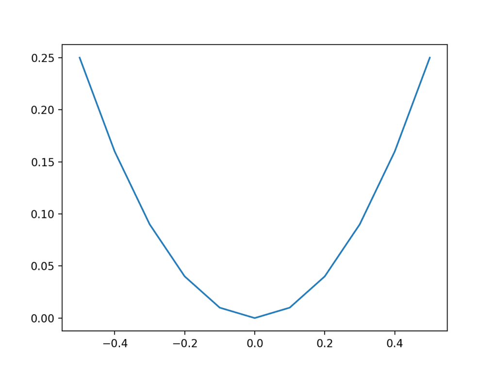
Plot of inputs vs. outputs for X^2 function.
We can generate random samples or points from the function.
This can be achieved by generating random values between -0.5 and 0.5 and calculating the associated output value. Repeating this many times will give a sample of points from the function, e.g. “real samples.”
Plotting these samples using a scatter plot will show the same u-shape plot, although comprised of the individual random samples.
The complete example is listed below.
Want to Develop GANs from Scratch?
Take my free 7-day email crash course now (with sample code).
Click to sign-up and also get a free PDF Ebook version of the course.
First, we generate uniformly random values between 0 and 1, then shift them to the range -0.5 and 0.5. We then calculate the output value for each randomly generated input value and combine the arrays into a single NumPy array with n rows (100) and two columns.
|
1 2 3 4 5 6 7 8 9 10 11 12 13 14 15 16 17 18 19 20 21 |
# example of generating random samples from X^2 from numpy.random import rand from numpy import hstack from matplotlib import pyplot # generate randoms sample from x^2 def generate_samples(n=100): # generate random inputs in [-0.5, 0.5] X1 = rand(n) - 0.5 # generate outputs X^2 (quadratic) X2 = X1 * X1 # stack arrays X1 = X1.reshape(n, 1) X2 = X2.reshape(n, 1) return hstack((X1, X2)) # generate samples data = generate_samples() # plot samples pyplot.scatter(data[:, 0], data[:, 1]) pyplot.show() |
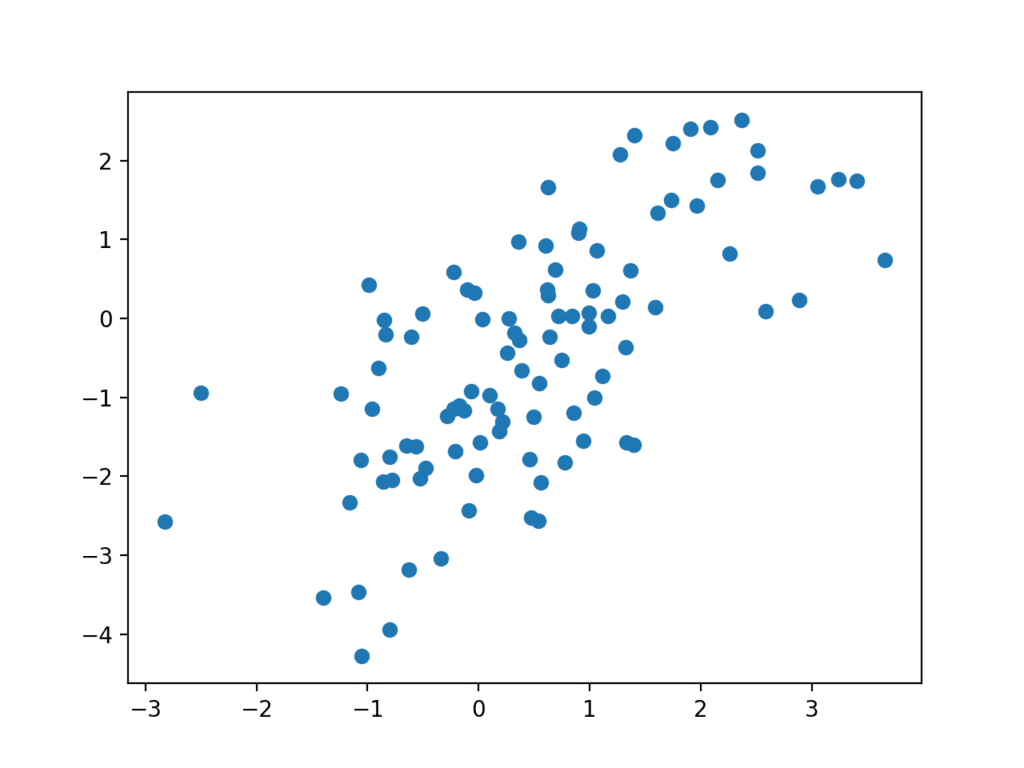
Running the example generates 100 random inputs and their calculated output and plots the sample as a scatter plot, showing the familiar u-shape.
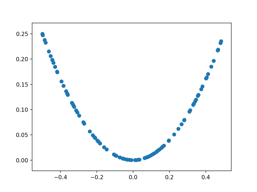
Plot of randomly generated sample of inputs vs. calculated outputs for X^2 function.
We can use this function as a starting point for generating real samples for our discriminator function. Specifically, a sample is comprised of a vector with two elements, one for the input and one for the output of our one-dimensional function.
We can also imagine how a generator model could generate new samples that we can plot and compare to the expected u-shape of the X^2 function. Specifically, a generator would output a vector with two elements: one for the input and one for the output of our one-dimensional function.
Define a Discriminator Model
The next step is to define the discriminator model.
The model must take a sample from our problem, such as a vector with two elements, and output a classification prediction as to whether the sample is real or fake.
This is a binary classification problem.
- Inputs: Sample with two real values.
- Outputs: Binary classification, likelihood the sample is real (or fake).
The problem is very simple, meaning that we don’t need a complex neural network to model it.
The discriminator model will have one hidden layer with 25 nodes and we will use the ReLU activation function and an appropriate weight initialization method called He weight initialization.
The output layer will have one node for the binary classification using the sigmoid activation function.
The model will minimize the binary cross entropy loss function, and the Adam version of stochastic gradient descent will be used because it is very effective.
The define_discriminator() function below defines and returns the discriminator model. The function parameterizes the number of inputs to expect, which defaults to two.
|
1 2 3 4 5 6 7 8 |
# define the standalone discriminator model def define_discriminator(n_inputs=2): model = Sequential() model.add(Dense(25, activation='relu', kernel_initializer='he_uniform', input_dim=n_inputs)) model.add(Dense(1, activation='sigmoid')) # compile model model.compile(loss='binary_crossentropy', optimizer='adam', metrics=['accuracy']) return model |
We can use this function to define the discriminator model and summarize it. The complete example is listed below.
|
1 2 3 4 5 6 7 8 9 10 11 12 13 14 15 16 17 18 19 20 |
# define the discriminator model from keras.models import Sequential from keras.layers import Dense from keras.utils.vis_utils import plot_model # define the standalone discriminator model def define_discriminator(n_inputs=2): model = Sequential() model.add(Dense(25, activation='relu', kernel_initializer='he_uniform', input_dim=n_inputs)) model.add(Dense(1, activation='sigmoid')) # compile model model.compile(loss='binary_crossentropy', optimizer='adam', metrics=['accuracy']) return model # define the discriminator model model = define_discriminator() # summarize the model model.summary() # plot the model plot_model(model, to_file='discriminator_plot.png', show_shapes=True, show_layer_names=True) |
Running the example defines the discriminator model and summarizes it.
|
1 2 3 4 5 6 7 8 9 10 11 |
_________________________________________________________________ Layer (type) Output Shape Param # ================================================================= dense_1 (Dense) (None, 25) 75 _________________________________________________________________ dense_2 (Dense) (None, 1) 26 ================================================================= Total params: 101 Trainable params: 101 Non-trainable params: 0 _________________________________________________________________ |
A plot of the model is also created and we can see that the model expects two inputs and will predict a single output.
Note: creating this plot assumes that the pydot and graphviz libraries are installed. If this is a problem, you can comment out the import statement for the plot_model function and the call to the plot_model() function.
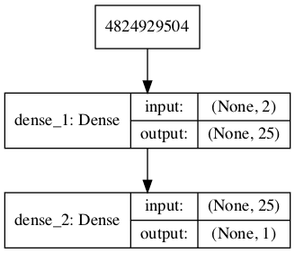
Plot of the Discriminator Model in the GAN
We could start training this model now with real examples with a class label of one and randomly generated samples with a class label of zero.
There is no need to do this, but the elements we will develop will be useful later, and it helps to see that the discriminator is just a normal neural network model.
First, we can update our generate_samples() function from the prediction section and call it generate_real_samples() and have it also return the output class labels for the real samples, specifically, an array of 1 values, where class=1 means real.
|
1 2 3 4 5 6 7 8 9 10 11 12 13 |
# generate n real samples with class labels def generate_real_samples(n): # generate inputs in [-0.5, 0.5] X1 = rand(n) - 0.5 # generate outputs X^2 X2 = X1 * X1 # stack arrays X1 = X1.reshape(n, 1) X2 = X2.reshape(n, 1) X = hstack((X1, X2)) # generate class labels y = ones((n, 1)) return X, y |
Next, we can create a copy of this function for creating fake examples.
In this case, we will generate random values in the range -1 and 1 for both elements of a sample. The output class label for all of these examples is 0.
This function will act as our fake generator model.
|
1 2 3 4 5 6 7 8 9 10 11 12 13 |
# generate n fake samples with class labels def generate_fake_samples(n): # generate inputs in [-1, 1] X1 = -1 + rand(n) * 2 # generate outputs in [-1, 1] X2 = -1 + rand(n) * 2 # stack arrays X1 = X1.reshape(n, 1) X2 = X2.reshape(n, 1) X = hstack((X1, X2)) # generate class labels y = zeros((n, 1)) return X, y |
Next, we need a function to train and evaluate the discriminator model.
This can be achieved by manually enumerating the training epochs and for each epoch generating a half batch of real examples and a half batch of fake examples, and updating the model on each, e.g. one whole batch of examples. The train() function could be used, but in this case, we will use the train_on_batch() function directly.
The model can then be evaluated on the generated examples and we can report the classification accuracy on the real and fake samples.
The train_discriminator() function below implements this, training the model for 1,000 batches and using 128 samples per batch (64 fake and 64 real).
|
1 2 3 4 5 6 7 8 9 10 11 12 13 14 15 16 17 |
# train the discriminator model def train_discriminator(model, n_epochs=1000, n_batch=128): half_batch = int(n_batch / 2) # run epochs manually for i in range(n_epochs): # generate real examples X_real, y_real = generate_real_samples(half_batch) # update model model.train_on_batch(X_real, y_real) # generate fake examples X_fake, y_fake = generate_fake_samples(half_batch) # update model model.train_on_batch(X_fake, y_fake) # evaluate the model _, acc_real = model.evaluate(X_real, y_real, verbose=0) _, acc_fake = model.evaluate(X_fake, y_fake, verbose=0) print(i, acc_real, acc_fake) |
We can tie all of this together and train the discriminator model on real and fake examples.
The complete example is listed below.
|
1 2 3 4 5 6 7 8 9 10 11 12 13 14 15 16 17 18 19 20 21 22 23 24 25 26 27 28 29 30 31 32 33 34 35 36 37 38 39 40 41 42 43 44 45 46 47 48 49 50 51 52 53 54 55 56 57 58 59 60 61 62 63 64 65 66 67 68 |
# define and fit a discriminator model from numpy import zeros from numpy import ones from numpy import hstack from numpy.random import rand from numpy.random import randn from keras.models import Sequential from keras.layers import Dense # define the standalone discriminator model def define_discriminator(n_inputs=2): model = Sequential() model.add(Dense(25, activation='relu', kernel_initializer='he_uniform', input_dim=n_inputs)) model.add(Dense(1, activation='sigmoid')) # compile model model.compile(loss='binary_crossentropy', optimizer='adam', metrics=['accuracy']) return model # generate n real samples with class labels def generate_real_samples(n): # generate inputs in [-0.5, 0.5] X1 = rand(n) - 0.5 # generate outputs X^2 X2 = X1 * X1 # stack arrays X1 = X1.reshape(n, 1) X2 = X2.reshape(n, 1) X = hstack((X1, X2)) # generate class labels y = ones((n, 1)) return X, y # generate n fake samples with class labels def generate_fake_samples(n): # generate inputs in [-1, 1] X1 = -1 + rand(n) * 2 # generate outputs in [-1, 1] X2 = -1 + rand(n) * 2 # stack arrays X1 = X1.reshape(n, 1) X2 = X2.reshape(n, 1) X = hstack((X1, X2)) # generate class labels y = zeros((n, 1)) return X, y # train the discriminator model def train_discriminator(model, n_epochs=1000, n_batch=128): half_batch = int(n_batch / 2) # run epochs manually for i in range(n_epochs): # generate real examples X_real, y_real = generate_real_samples(half_batch) # update model model.train_on_batch(X_real, y_real) # generate fake examples X_fake, y_fake = generate_fake_samples(half_batch) # update model model.train_on_batch(X_fake, y_fake) # evaluate the model _, acc_real = model.evaluate(X_real, y_real, verbose=0) _, acc_fake = model.evaluate(X_fake, y_fake, verbose=0) print(i, acc_real, acc_fake) # define the discriminator model model = define_discriminator() # fit the model train_discriminator(model) |
Running the example generates real and fake examples and updates the model, then evaluates the model on the same examples and prints the classification accuracy.
Note: Your results may vary given the stochastic nature of the algorithm or evaluation procedure, or differences in numerical precision. Consider running the example a few times and compare the average outcome.
In this case, the model rapidly learns to correctly identify the real examples with perfect accuracy and is very good at identifying the fake examples with 80% to 90% accuracy.
|
1 2 3 4 5 6 |
... 995 1.0 0.875 996 1.0 0.921875 997 1.0 0.859375 998 1.0 0.9375 999 1.0 0.8125 |
Training the discriminator model is straightforward. The goal is to train a generator model, not a discriminator model, and that is where the complexity of GANs truly lies.
Define a Generator Model
The next step is to define the generator model.
The generator model takes as input a point from the latent space and generates a new sample, e.g. a vector with both the input and output elements of our function, e.g. x and x^2.
A latent variable is a hidden or unobserved variable, and a latent space is a multi-dimensional vector space of these variables. We can define the size of the latent space for our problem and the shape or distribution of variables in the latent space.
This is because the latent space has no meaning until the generator model starts assigning meaning to points in the space as it learns. After training, points in the latent space will correspond to points in the output space, e.g. in the space of generated samples.
We will define a small latent space of five dimensions and use the standard approach in the GAN literature of using a Gaussian distribution for each variable in the latent space. We will generate new inputs by drawing random numbers from a standard Gaussian distribution, i.e. mean of zero and a standard deviation of one.
- Inputs: Point in latent space, e.g. a five-element vector of Gaussian random numbers.
- Outputs: Two-element vector representing a generated sample for our function (x and x^2).
The generator model will be small like the discriminator model.
It will have a single hidden layer with five nodes and will use the ReLU activation function and the He weight initialization. The output layer will have two nodes for the two elements in a generated vector and will use a linear activation function.
A linear activation function is used because we know we want the generator to output a vector of real values and the scale will be [-0.5, 0.5] for the first element and about [0.0, 0.25] for the second element.
The model is not compiled. The reason for this is that the generator model is not fit directly.
The define_generator() function below defines and returns the generator model.
The size of the latent dimension is parameterized in case we want to play with it later, and the output shape of the model is also parameterized, matching the function for defining the discriminator model.
|
1 2 3 4 5 6 |
# define the standalone generator model def define_generator(latent_dim, n_outputs=2): model = Sequential() model.add(Dense(15, activation='relu', kernel_initializer='he_uniform', input_dim=latent_dim)) model.add(Dense(n_outputs, activation='linear')) return model |
We can summarize the model to help better understand the input and output shapes.
The complete example is listed below.
|
1 2 3 4 5 6 7 8 9 10 11 12 13 14 15 16 17 18 |
# define the generator model from keras.models import Sequential from keras.layers import Dense from keras.utils.vis_utils import plot_model # define the standalone generator model def define_generator(latent_dim, n_outputs=2): model = Sequential() model.add(Dense(15, activation='relu', kernel_initializer='he_uniform', input_dim=latent_dim)) model.add(Dense(n_outputs, activation='linear')) return model # define the discriminator model model = define_generator(5) # summarize the model model.summary() # plot the model plot_model(model, to_file='generator_plot.png', show_shapes=True, show_layer_names=True) |
Running the example defines the generator model and summarizes it.
|
1 2 3 4 5 6 7 8 9 10 11 |
_________________________________________________________________ Layer (type) Output Shape Param # ================================================================= dense_1 (Dense) (None, 15) 90 _________________________________________________________________ dense_2 (Dense) (None, 2) 32 ================================================================= Total params: 122 Trainable params: 122 Non-trainable params: 0 _________________________________________________________________ |
A plot of the model is also created and we can see that the model expects a five-element point from the latent space as input and will predict a two-element vector as output.
Note: creating this plot assumes that the pydot and graphviz libraries are installed. If this is a problem, you can comment out the import statement for the plot_model function and the call to the plot_model() function.
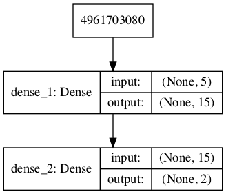
Plot of the Generator Model in the GAN
We can see that the model takes as input a random five-element vector from the latent space and outputs a two-element vector for our one-dimensional function.
This model cannot do much at the moment. Nevertheless, we can demonstrate how to use it to generate samples. This is not needed, but again, some of these elements may be useful later.
The first step is to generate new points in the latent space. We can achieve this by calling the randn() NumPy function for generating arrays of random numbers drawn from a standard Gaussian.
The array of random numbers can then be reshaped into samples: that is n rows with five elements per row. The generate_latent_points() function below implements this and generates the desired number of points in the latent space that can be used as input to the generator model.
|
1 2 3 4 5 6 7 |
# generate points in latent space as input for the generator def generate_latent_points(latent_dim, n): # generate points in the latent space x_input = randn(latent_dim * n) # reshape into a batch of inputs for the network x_input = x_input.reshape(n, latent_dim) return x_input |
Next, we can use the generated points as input the generator model to generate new samples, then plot the samples.
The generate_fake_samples() function below implements this, where the defined generator and size of the latent space are passed as arguments, along with the number of points for the model to generate.
|
1 2 3 4 5 6 7 8 9 |
# use the generator to generate n fake examples and plot the results def generate_fake_samples(generator, latent_dim, n): # generate points in latent space x_input = generate_latent_points(latent_dim, n) # predict outputs X = generator.predict(x_input) # plot the results pyplot.scatter(X[:, 0], X[:, 1]) pyplot.show() |
Tying this together, the complete example is listed below.
|
1 2 3 4 5 6 7 8 9 10 11 12 13 14 15 16 17 18 19 20 21 22 23 24 25 26 27 28 29 30 31 32 33 34 35 36 37 |
# define and use the generator model from numpy.random import randn from keras.models import Sequential from keras.layers import Dense from matplotlib import pyplot # define the standalone generator model def define_generator(latent_dim, n_outputs=2): model = Sequential() model.add(Dense(15, activation='relu', kernel_initializer='he_uniform', input_dim=latent_dim)) model.add(Dense(n_outputs, activation='linear')) return model # generate points in latent space as input for the generator def generate_latent_points(latent_dim, n): # generate points in the latent space x_input = randn(latent_dim * n) # reshape into a batch of inputs for the network x_input = x_input.reshape(n, latent_dim) return x_input # use the generator to generate n fake examples and plot the results def generate_fake_samples(generator, latent_dim, n): # generate points in latent space x_input = generate_latent_points(latent_dim, n) # predict outputs X = generator.predict(x_input) # plot the results pyplot.scatter(X[:, 0], X[:, 1]) pyplot.show() # size of the latent space latent_dim = 5 # define the discriminator model model = define_generator(latent_dim) # generate and plot generated samples generate_fake_samples(model, latent_dim, 100) |
Running the example generates 100 random points from the latent space, uses this as input to the generator and generates 100 fake samples from our one-dimensional function domain.
As the generator has not been trained, the generated points are complete rubbish, as we expect, but we can imagine that as the model is trained, these points will slowly begin to resemble the target function and its u-shape.
Scatter plot of Fake Samples Predicted by the Generator Model.
We have now seen how to define and use the generator model. We will need to use the generator model in this way to create samples for the discriminator to classify.
We have not seen how the generator model is trained; that is next.
Training the Generator Model
The weights in the generator model are updated based on the performance of the discriminator model.
When the discriminator is good at detecting fake samples, the generator is updated more, and when the discriminator model is relatively poor or confused when detecting fake samples, the generator model is updated less.
This defines the zero-sum or adversarial relationship between these two models.
There may be many ways to implement this using the Keras API, but perhaps the simplest approach is to create a new model that subsumes or encapsulates the generator and discriminator models.
Specifically, a new GAN model can be defined that stacks the generator and discriminator such that the generator receives as input random points in the latent space, generates samples that are fed into the discriminator model directly, classified, and the output of this larger model can be used to update the model weights of the generator.
To be clear, we are not talking about a new third model, just a logical third model that uses the already-defined layers and weights from the standalone generator and discriminator models.
Only the discriminator is concerned with distinguishing between real and fake examples; therefore, the discriminator model can be trained in a standalone manner on examples of each.
The generator model is only concerned with the discriminator’s performance on fake examples. Therefore, we will mark all of the layers in the discriminator as not trainable when it is part of the GAN model so that they can not be updated and overtrained on fake examples.
When training the generator via this subsumed GAN model, there is one more important change. We want the discriminator to think that the samples output by the generator are real, not fake. Therefore, when the generator is trained as part of the GAN model, we will mark the generated samples as real (class 1).
We can imagine that the discriminator will then classify the generated samples as not real (class 0) or a low probability of being real (0.3 or 0.5). The backpropagation process used to update the model weights will see this as a large error and will update the model weights (i.e. only the weights in the generator) to correct for this error, in turn making the generator better at generating plausible fake samples.
Let’s make this concrete.
- Inputs: Point in latent space, e.g. a five-element vector of Gaussian random numbers.
- Outputs: Binary classification, likelihood the sample is real (or fake).
The define_gan() function below takes as arguments the already-defined generator and discriminator models and creates the new logical third model subsuming these two models. The weights in the discriminator are marked as not trainable, which only affects the weights as seen by the GAN model and not the standalone discriminator model.
The GAN model then uses the same binary cross entropy loss function as the discriminator and the efficient Adam version of stochastic gradient descent.
|
1 2 3 4 5 6 7 8 9 10 11 12 13 |
# define the combined generator and discriminator model, for updating the generator def define_gan(generator, discriminator): # make weights in the discriminator not trainable discriminator.trainable = False # connect them model = Sequential() # add generator model.add(generator) # add the discriminator model.add(discriminator) # compile model model.compile(loss='binary_crossentropy', optimizer='adam') return model |
Making the discriminator not trainable is a clever trick in the Keras API.
The trainable property impacts the model when it is compiled. The discriminator model was compiled with trainable layers, therefore the model weights in those layers will be updated when the standalone model is updated via calls to train_on_batch().
The discriminator model was marked as not trainable, added to the GAN model, and compiled. In this model, the model weights of the discriminator model are not trainable and cannot be changed when the GAN model is updated via calls to train_on_batch().
This behavior is described in the Keras API documentation here:
The complete example of creating the discriminator, generator, and composite model is listed below.
|
1 2 3 4 5 6 7 8 9 10 11 12 13 14 15 16 17 18 19 20 21 22 23 24 25 26 27 28 29 30 31 32 33 34 35 36 37 38 39 40 41 42 43 44 45 46 47 |
# demonstrate creating the three models in the gan from keras.models import Sequential from keras.layers import Dense from keras.utils.vis_utils import plot_model # define the standalone discriminator model def define_discriminator(n_inputs=2): model = Sequential() model.add(Dense(25, activation='relu', kernel_initializer='he_uniform', input_dim=n_inputs)) model.add(Dense(1, activation='sigmoid')) # compile model model.compile(loss='binary_crossentropy', optimizer='adam', metrics=['accuracy']) return model # define the standalone generator model def define_generator(latent_dim, n_outputs=2): model = Sequential() model.add(Dense(15, activation='relu', kernel_initializer='he_uniform', input_dim=latent_dim)) model.add(Dense(n_outputs, activation='linear')) return model # define the combined generator and discriminator model, for updating the generator def define_gan(generator, discriminator): # make weights in the discriminator not trainable discriminator.trainable = False # connect them model = Sequential() # add generator model.add(generator) # add the discriminator model.add(discriminator) # compile model model.compile(loss='binary_crossentropy', optimizer='adam') return model # size of the latent space latent_dim = 5 # create the discriminator discriminator = define_discriminator() # create the generator generator = define_generator(latent_dim) # create the gan gan_model = define_gan(generator, discriminator) # summarize gan model gan_model.summary() # plot gan model plot_model(gan_model, to_file='gan_plot.png', show_shapes=True, show_layer_names=True) |
Running the example first creates a summary of the composite model.
|
1 2 3 4 5 6 7 8 9 10 11 |
_________________________________________________________________ Layer (type) Output Shape Param # ================================================================= sequential_2 (Sequential) (None, 2) 122 _________________________________________________________________ sequential_1 (Sequential) (None, 1) 101 ================================================================= Total params: 223 Trainable params: 122 Non-trainable params: 101 _________________________________________________________________ |
A plot of the model is also created and we can see that the model expects a five-element point in latent space as input and will predict a single output classification label.
Note, creating this plot assumes that the pydot and graphviz libraries are installed. If this is a problem, you can comment out the import statement for the plot_model function and the call to the plot_model() function.
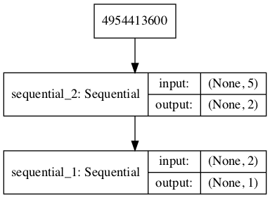
Plot of the Composite Generator and Discriminator Model in the GAN
Training the composite model involves generating a batch-worth of points in the latent space via the generate_latent_points() function in the previous section, and class=1 labels and calling the train_on_batch() function.
The train_gan() function below demonstrates this, although it is pretty uninteresting as only the generator will be updated each epoch, leaving the discriminator with default model weights.
|
1 2 3 4 5 6 7 8 9 10 |
# train the composite model def train_gan(gan_model, latent_dim, n_epochs=10000, n_batch=128): # manually enumerate epochs for i in range(n_epochs): # prepare points in latent space as input for the generator x_gan = generate_latent_points(latent_dim, n_batch) # create inverted labels for the fake samples y_gan = ones((n_batch, 1)) # update the generator via the discriminator's error gan_model.train_on_batch(x_gan, y_gan) |
Instead, what is required is that we first update the discriminator model with real and fake samples, then update the generator via the composite model.
This requires combining elements from the train_discriminator() function defined in the discriminator section and the train_gan() function defined above. It also requires that the generate_fake_samples() function use the generator model to generate fake samples instead of generating random numbers.
The complete train function for updating the discriminator model and the generator (via the composite model) is listed below.
|
1 2 3 4 5 6 7 8 9 10 11 12 13 14 15 16 17 18 19 |
# train the generator and discriminator def train(g_model, d_model, gan_model, latent_dim, n_epochs=10000, n_batch=128): # determine half the size of one batch, for updating the discriminator half_batch = int(n_batch / 2) # manually enumerate epochs for i in range(n_epochs): # prepare real samples x_real, y_real = generate_real_samples(half_batch) # prepare fake examples x_fake, y_fake = generate_fake_samples(g_model, latent_dim, half_batch) # update discriminator d_model.train_on_batch(x_real, y_real) d_model.train_on_batch(x_fake, y_fake) # prepare points in latent space as input for the generator x_gan = generate_latent_points(latent_dim, n_batch) # create inverted labels for the fake samples y_gan = ones((n_batch, 1)) # update the generator via the discriminator's error gan_model.train_on_batch(x_gan, y_gan) |
We almost have everything we need to develop a GAN for our one-dimensional function.
One remaining aspect is the evaluation of the model.
Evaluating the Performance of the GAN
Generally, there are no objective ways to evaluate the performance of a GAN model.
In this specific case, we can devise an objective measure for the generated samples as we know the true underlying input domain and target function and can calculate an objective error measure.
Nevertheless, we will not calculate this objective error score in this tutorial. Instead, we will use the subjective approach used in most GAN applications. Specifically, we will use the generator to generate new samples and inspect them relative to real samples from the domain.
First, we can use the generate_real_samples() function developed in the discriminator part above to generate real examples. Creating a scatter plot of these examples will create the familiar u-shape of our target function.
|
1 2 3 4 5 6 7 8 9 10 11 12 13 |
# generate n real samples with class labels def generate_real_samples(n): # generate inputs in [-0.5, 0.5] X1 = rand(n) - 0.5 # generate outputs X^2 X2 = X1 * X1 # stack arrays X1 = X1.reshape(n, 1) X2 = X2.reshape(n, 1) X = hstack((X1, X2)) # generate class labels y = ones((n, 1)) return X, y |
Next, we can use the generator model to generate the same number of fake samples.
This requires first generating the same number of points in the latent space via the generate_latent_points() function developed in the generator section above. These can then be passed to the generator model and used to generate samples that can also be plotted on the same scatter plot.
|
1 2 3 4 5 6 7 |
# generate points in latent space as input for the generator def generate_latent_points(latent_dim, n): # generate points in the latent space x_input = randn(latent_dim * n) # reshape into a batch of inputs for the network x_input = x_input.reshape(n, latent_dim) return x_input |
The generate_fake_samples() function below generates these fake samples and the associated class label of 0 which will be useful later.
|
1 2 3 4 5 6 7 8 9 |
# use the generator to generate n fake examples, with class labels def generate_fake_samples(generator, latent_dim, n): # generate points in latent space x_input = generate_latent_points(latent_dim, n) # predict outputs X = generator.predict(x_input) # create class labels y = zeros((n, 1)) return X, y |
Having both samples plotted on the same graph allows them to be directly compared to see if the same input and output domain are covered and whether the expected shape of the target function has been appropriately captured, at least subjectively.
The summarize_performance() function below can be called any time during training to create a scatter plot of real and generated points to get an idea of the current capability of the generator model.
|
1 2 3 4 5 6 7 8 9 10 |
# plot real and fake points def summarize_performance(generator, latent_dim, n=100): # prepare real samples x_real, y_real = generate_real_samples(n) # prepare fake examples x_fake, y_fake = generate_fake_samples(generator, latent_dim, n) # scatter plot real and fake data points pyplot.scatter(x_real[:, 0], x_real[:, 1], color='red') pyplot.scatter(x_fake[:, 0], x_fake[:, 1], color='blue') pyplot.show() |
We may also be interested in the performance of the discriminator model at the same time.
Specifically, we are interested to know how well the discriminator model can correctly identify real and fake samples. A good generator model should make the discriminator model confused, resulting in a classification accuracy closer to 50% on real and fake examples.
We can update the summarize_performance() function to also take the discriminator and current epoch number as arguments and report the accuracy on the sample of real and fake examples.
|
1 2 3 4 5 6 7 8 9 10 11 12 13 14 15 16 |
# evaluate the discriminator and plot real and fake points def summarize_performance(epoch, generator, discriminator, latent_dim, n=100): # prepare real samples x_real, y_real = generate_real_samples(n) # evaluate discriminator on real examples _, acc_real = discriminator.evaluate(x_real, y_real, verbose=0) # prepare fake examples x_fake, y_fake = generate_fake_samples(generator, latent_dim, n) # evaluate discriminator on fake examples _, acc_fake = discriminator.evaluate(x_fake, y_fake, verbose=0) # summarize discriminator performance print(epoch, acc_real, acc_fake) # scatter plot real and fake data points pyplot.scatter(x_real[:, 0], x_real[:, 1], color='red') pyplot.scatter(x_fake[:, 0], x_fake[:, 1], color='blue') pyplot.show() |
This function can then be called periodically during training.
For example, if we choose to train the models for 10,000 iterations, it may be interesting to check-in on the performance of the model every 2,000 iterations.
We can achieve this by parameterizing the frequency of the check-in via n_eval argument, and calling the summarize_performance() function from the train() function after the appropriate number of iterations.
The updated version of the train() function with this change is listed below.
|
1 2 3 4 5 6 7 8 9 10 11 12 13 14 15 16 17 18 19 20 21 22 |
# train the generator and discriminator def train(g_model, d_model, gan_model, latent_dim, n_epochs=10000, n_batch=128, n_eval=2000): # determine half the size of one batch, for updating the discriminator half_batch = int(n_batch / 2) # manually enumerate epochs for i in range(n_epochs): # prepare real samples x_real, y_real = generate_real_samples(half_batch) # prepare fake examples x_fake, y_fake = generate_fake_samples(g_model, latent_dim, half_batch) # update discriminator d_model.train_on_batch(x_real, y_real) d_model.train_on_batch(x_fake, y_fake) # prepare points in latent space as input for the generator x_gan = generate_latent_points(latent_dim, n_batch) # create inverted labels for the fake samples y_gan = ones((n_batch, 1)) # update the generator via the discriminator's error gan_model.train_on_batch(x_gan, y_gan) # evaluate the model every n_eval epochs if (i+1) % n_eval == 0: summarize_performance(i, g_model, d_model, latent_dim) |
Complete Example of Training the GAN
We now have everything we need to train and evaluate a GAN on our chosen one-dimensional function.
The complete example is listed below.
|
1 2 3 4 5 6 7 8 9 10 11 12 13 14 15 16 17 18 19 20 21 22 23 24 25 26 27 28 29 30 31 32 33 34 35 36 37 38 39 40 41 42 43 44 45 46 47 48 49 50 51 52 53 54 55 56 57 58 59 60 61 62 63 64 65 66 67 68 69 70 71 72 73 74 75 76 77 78 79 80 81 82 83 84 85 86 87 88 89 90 91 92 93 94 95 96 97 98 99 100 101 102 103 104 105 106 107 108 109 110 111 112 113 114 115 116 117 118 119 120 121 122 |
# train a generative adversarial network on a one-dimensional function from numpy import hstack from numpy import zeros from numpy import ones from numpy.random import rand from numpy.random import randn from keras.models import Sequential from keras.layers import Dense from matplotlib import pyplot # define the standalone discriminator model def define_discriminator(n_inputs=2): model = Sequential() model.add(Dense(25, activation='relu', kernel_initializer='he_uniform', input_dim=n_inputs)) model.add(Dense(1, activation='sigmoid')) # compile model model.compile(loss='binary_crossentropy', optimizer='adam', metrics=['accuracy']) return model # define the standalone generator model def define_generator(latent_dim, n_outputs=2): model = Sequential() model.add(Dense(15, activation='relu', kernel_initializer='he_uniform', input_dim=latent_dim)) model.add(Dense(n_outputs, activation='linear')) return model # define the combined generator and discriminator model, for updating the generator def define_gan(generator, discriminator): # make weights in the discriminator not trainable discriminator.trainable = False # connect them model = Sequential() # add generator model.add(generator) # add the discriminator model.add(discriminator) # compile model model.compile(loss='binary_crossentropy', optimizer='adam') return model # generate n real samples with class labels def generate_real_samples(n): # generate inputs in [-0.5, 0.5] X1 = rand(n) - 0.5 # generate outputs X^2 X2 = X1 * X1 # stack arrays X1 = X1.reshape(n, 1) X2 = X2.reshape(n, 1) X = hstack((X1, X2)) # generate class labels y = ones((n, 1)) return X, y # generate points in latent space as input for the generator def generate_latent_points(latent_dim, n): # generate points in the latent space x_input = randn(latent_dim * n) # reshape into a batch of inputs for the network x_input = x_input.reshape(n, latent_dim) return x_input # use the generator to generate n fake examples, with class labels def generate_fake_samples(generator, latent_dim, n): # generate points in latent space x_input = generate_latent_points(latent_dim, n) # predict outputs X = generator.predict(x_input) # create class labels y = zeros((n, 1)) return X, y # evaluate the discriminator and plot real and fake points def summarize_performance(epoch, generator, discriminator, latent_dim, n=100): # prepare real samples x_real, y_real = generate_real_samples(n) # evaluate discriminator on real examples _, acc_real = discriminator.evaluate(x_real, y_real, verbose=0) # prepare fake examples x_fake, y_fake = generate_fake_samples(generator, latent_dim, n) # evaluate discriminator on fake examples _, acc_fake = discriminator.evaluate(x_fake, y_fake, verbose=0) # summarize discriminator performance print(epoch, acc_real, acc_fake) # scatter plot real and fake data points pyplot.scatter(x_real[:, 0], x_real[:, 1], color='red') pyplot.scatter(x_fake[:, 0], x_fake[:, 1], color='blue') pyplot.show() # train the generator and discriminator def train(g_model, d_model, gan_model, latent_dim, n_epochs=10000, n_batch=128, n_eval=2000): # determine half the size of one batch, for updating the discriminator half_batch = int(n_batch / 2) # manually enumerate epochs for i in range(n_epochs): # prepare real samples x_real, y_real = generate_real_samples(half_batch) # prepare fake examples x_fake, y_fake = generate_fake_samples(g_model, latent_dim, half_batch) # update discriminator d_model.train_on_batch(x_real, y_real) d_model.train_on_batch(x_fake, y_fake) # prepare points in latent space as input for the generator x_gan = generate_latent_points(latent_dim, n_batch) # create inverted labels for the fake samples y_gan = ones((n_batch, 1)) # update the generator via the discriminator's error gan_model.train_on_batch(x_gan, y_gan) # evaluate the model every n_eval epochs if (i+1) % n_eval == 0: summarize_performance(i, g_model, d_model, latent_dim) # size of the latent space latent_dim = 5 # create the discriminator discriminator = define_discriminator() # create the generator generator = define_generator(latent_dim) # create the gan gan_model = define_gan(generator, discriminator) # train model train(generator, discriminator, gan_model, latent_dim) |
Running the example reports model performance every 2,000 training iterations (batches) and creates a plot.
Note: Your results may vary given the stochastic nature of the algorithm or evaluation procedure, or differences in numerical precision. Consider running the example a few times and compare the average outcome.
We can see that the training process is relatively unstable. The first column reports the iteration number, the second the classification accuracy of the discriminator for real examples, and the third column the classification accuracy of the discriminator for generated (fake) examples.
In this case, we can see that the discriminator remains relatively confused about real examples, and performance on identifying fake examples varies.
|
1 2 3 4 5 |
1999 0.45 1.0 3999 0.45 0.91 5999 0.86 0.16 7999 0.6 0.41 9999 0.15 0.93 |
I will omit providing the five created plots here for brevity; instead we will look at only two.
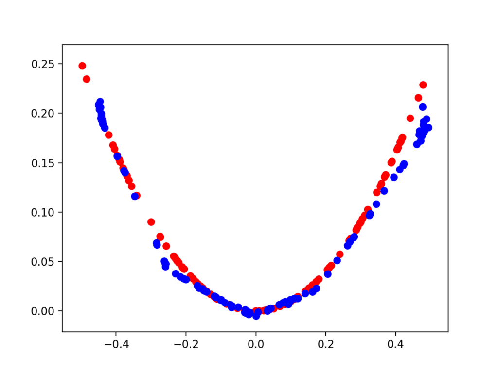
The first plot is created after 2,000 iterations and shows real (red) vs. fake (blue) samples. The model performs poorly initially with a cluster of generated points only in the positive input domain, although with the right functional relationship.
Scatter Plot of Real and Generated Examples for the Target Function After 2,000 Iterations.
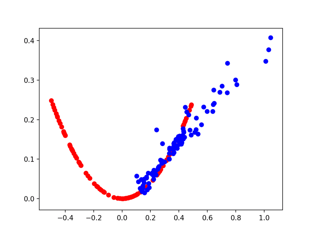
The second plot shows real (red) vs. fake (blue) after 10,000 iterations.
Here we can see that the generator model does a reasonable job of generating plausible samples, with the input values in the right domain between [-0.5 and 0.5] and the output values showing the X^2 relationship, or close to it.
Scatter Plot of Real and Generated Examples for the Target Function After 10,000 Iterations.
Extensions
This section lists some ideas for extending the tutorial that you may wish to explore.
- Model Architecture. Experiment with alternate model architectures for the discriminator and generator, such as more or fewer nodes, layers, and alternate activation functions such as leaky ReLU.
- Data Scaling. Experiment with alternate activation functions such as the hyperbolic tangent (tanh) and any required scaling of training data.
- Alternate Target Function. Experiment with an alternate target function, such a simple sine wave, Gaussian distribution, a different quadratic, or even a multi-modal polynomial function.
If you explore any of these extensions, I’d love to know.
Post your findings in the comments below.
Further Reading
This section provides more resources on the topic if you are looking to go deeper.
API
- Keras API
- How can I “freeze” Keras layers?
- MatplotLib API
- numpy.random.rand API
- numpy.random.randn API
- numpy.zeros API
- numpy.ones API
- numpy.hstack API
Summary
In this tutorial, you discovered how to develop a generative adversarial network from scratch for a one-dimensional function.
Specifically, you learned:
- The benefit of developing a generative adversarial network from scratch for a simple one-dimensional function.
- How to develop separate discriminator and generator models, as well as a composite model for training the generator via the discriminator’s predictive behavior.
- How to subjectively evaluate generated samples in the context of real examples from the problem domain.
Do you have any questions?
Ask your questions in the comments below and I will do my best to answer.
Develop Generative Adversarial Networks Today!
Develop Your GAN Models in Minutes
...with just a few lines of python codeDiscover how in my new Ebook:
Generative Adversarial Networks with Python
It provides self-study tutorials and end-to-end projects on:
DCGAN, conditional GANs, image translation, Pix2Pix, CycleGAN
and much more...
 in Keras")
 From Scratch")


Fantastic
Thanks!
Can you give some example using 2D convolution layers.
Yes, I have many examples scheduled.
I would be very interested in these examples too. Great post Jason, many thanks
There are many, a good place to start is here:
https://machinelearningmastery.com/how-to-develop-a-generative-adversarial-network-for-an-mnist-handwritten-digits-from-scratch-in-keras/
Dear Jason,
great tutorial as always! may i know if there would be any tuorial of using gan to generate time series data? I am really looking forward to that 🙂
best,
fan
I believe there are papers on the topic, I have not written a tutorial on the topic yet.
Thank you so much, I finally understood the magic behind GANs today. I’ve tried to understand that completely a few times in the past and have failed.
Thanks, I’m glad it helped!
Great post. Thanks Jason.
Naive question, how do you the trained model to generate more fake data? Or I am missing something 🙂
Great question.
Once the generator model is fit, you can call it all day long with new points from the latent space to generate new output points in the target domain.
Hi Jason
Thanks for this excellent post.
Are you planning to release GAN about pictures?
Yes, I have many great examples coming.
The first round with the descriminator you have actual real/fake criteria, namely f(x)==x^2. So sometimes the fake data will actually fall on this line. Is this an issue? What about the domain/range of the Generator, is there anything to keep it from narrowing it’s domain/range?
I read this pretty quickly, and Ill look more thoroughly in the near future. Thanks, great article.
Not sure I follow Matt, sorry. Are you able to elaborate?
The first question regards a rare occurance, but what about when your random generated data is exactly the same as real data. eg. x=0.2 and y=0.04.
The second quesiton is, could the generator learn to create outputs only for a limited range of x E [0,0.5] and never produce a negative x?
Randomly generating real obs is very rare. E.g. randomly generate pixels and get a face? Impossible.
I don’t see how it could matter, do you have something specific in mind?
For sure, we have complete control over the models involved. It is common to “play games” with the latent space, e.g. sample a narrow band during training then a wide band during inference to get more variety (in images).
Theoretically, the possibility exists, practically it is zero.
Hello jason,
You wrote : “The generator model will be small like the discriminator model. It will have a single hidden layer with five nodes
but it seems that you define a model with 15 nodes
model.add(Dense(15, activation=’relu’, kernel_initializer=’he_uniform’, input_dim=latent_dim))
the latent-dim parameter is not used
Am I wrong ?
Best
Yes, one layer, 15 nodes and “latent_dim” defines the input shape.
Hello jason
I was wrong, sorry
Best
No problem.
Sir, pls i am confused, how is backpropagation done in the generator, looking at the generator, it outputs a vector and the vector is passed into the discriminator for prediction but the discriminator outputs a scalar value, so how do we update the weights of the generator.
Good question, this may help:
https://machinelearningmastery.com/how-to-code-the-generative-adversarial-network-training-algorithm-and-loss-functions/
Thank you Jason. Very impressive.
Hello Jason
I tried with more hidden layer for the discriminator and with the LeakyReLu activation (see below)
It seems the tthe reuslts are a littel bit mor stable
Best
Nice work!
Hello Jason
some examples of the results I got with this more densed architecture
1999 0.9 0.9
3999 0.93 0.73
5999 0.8 0.98
7999 0.83 0.98
9999 0.82 0.97
Thanks for sharing Minel!
Thank you very much for this great post
Kindly elaborate more why you optionaly selected a latent space of dimension 5.
What will be the impact if you use let us say 10 , 20, 50 or even 100 instead of 5
It is arbitrary and not optimal.
You can experiment with diffrent sizes.
Hello Jason
Thank you very much for this article , I would like to use GAN for image colorization.
Could you tell me please, what is the important articles that may help me to start ?
I don’t have a tutorial on this topic, but I hope to cover it in the future.
Hello Jason
Why did it go wrong when I trained the discriminator? The error occurs in model.train_on_batch(X_real, y_real). It is InternalError: Failed to create session.
The error suggests you may have a problem with your development environment.
Perhaps try re-installing tensorflow?
The *trainable* property impacts the model when it is compiled. **The discriminator model** was compiled with trainable layers, therefore the model weights in those layers will be updated when the standalone model is updated via calls to *train_on_batch()*.
The discriminator should be replaced with the generator, right?
No, it is stated correctly I believe.
The weights are trainable in the discriminator, and not trainable when the discriminator is part of the composite model.
Thank you very much. I get it.
No problem.
Really nice job.
Do you mind if I use some of your code for my youtube videos.
I am currently learning about GAN’s and making videos helps me
reinforce what I have learned and forces me to look up things I don’t understand. Your tutorials are very helpful.
I will provide your link as well as let everyone know about your website.
Thank you so much for your blogs.
I rather you didn’t.
Thanks Jason,
Why didn’t you compile the generator the same way you have done with the discriminator?
Can the generator model predict without being compiled?
No need. The generator is not being fit directly.
i want to know how the model look like when we aggregate two model in a single one, like what you have done in define_gan ????
What do you mean how it looks?
You can use summary() or plot_model().
Hi Jason,
I am a big fan of your tutorials!
Not sure if you have already stated it in the Q/A, but what is the way to generate more data from the final Generative model?
I think I got it.
Please let me know if this is correct.
After training, I have a
generatormodel ready.n=100
x,_=generate_fake_samples(generator, latent_dim, n)
Looks good.
Thanks!
You can save the generator and then call model.predict() with points from the latent space to generate new examples.
I give many examples of this, perhaps start here:
https://machinelearningmastery.com/start-here/#gans
Hi Jason, Thank you for this simple, clear and fantastic post. I was searching for how to use GANs to model numeric data and this post really helped me. I applied the implementation here to my problem dataset and got it working, though I am not getting expected results. You can see the implementation in this Google Colab Notebook:
https://colab.research.google.com/drive/1erOPC6w9szqVDX9oU6gJfE88N1y1Tfwf
The dataset in my case is very sparse containing only some 34 data points from a lab test. My goal is to use GANs to synthesise more data points that match this lab test data distribution. I noticed during the training that sometimes randomly in some epoch, the accuracy reaches the equilibrium point of around 0.5 but still, all the fake points are not close to the real data. I tried varying the
batch sizeandnr_samplesin thetrainandsummarize_performancefunctions but I am not getting good results. I am not sure what else to try. Should I use higherlatent_dimor increase the layers and neurons in the generator or discriminator model?1.) Could you please take a look at the Google Colab notebook and give me some pointers on how to go about improving the quality of the synthesized data?
2.) In the scatter plot I just plotted the two most important variables (Xf and Xr_y) as I know there is a strong correlation between the two. But, for my multivariate data how do I actually ascertain whether the synthetic data from the GANs is valid?
Thanks!
I’m eager to help, but I don’t have the capacity to review/debug your code.
You can learn how to diagnose GAN problems here:
https://machinelearningmastery.com/practical-guide-to-gan-failure-modes/
And fix GAN problems here:
https://machinelearningmastery.com/how-to-code-generative-adversarial-network-hacks/
Hi Jason,
Thanks for pointing out to your other fantastic and useful posts. From your GAN failure modes post,I understood how to plot disc and gen losses to infer more about the GAN model performance. The accuracy score printed by
dmodel.train_on_batch(x,y)is different from the accuracy score printed bydiscriminator.evaluate(x,y)d_loss1, d_acc1 = d_model.train_on_batch(x_real, y_real)
d_loss2, d_acc2 = d_model.train_on_batch(x_fake, y_fake)
The above code prints the line:
Epoch:1999, disc_loss_real=0.693, disc_loss_fake=0.695 gen_loss=0.693, disc_acc_real=64, disc_acc_fake=37
_, acc_real = discriminator.evaluate(x_real, y_real, verbose=0)

_, acc_fake = discriminator.evaluate(x_fake, y_fake, verbose=0)
The above code prints the line:
Epoch:1999 Accuracy(RealData): 0.64 Accuracy(FakeData): 0.47
In a training iteration for 10,000 epochs for generating this U-shaped function,sometimes the acccuracy scores in the two lines match partially and other times they are completely different.
Epoch:1999, disc_loss_real=0.693, disc_loss_fake=0.695 gen_loss=0.693, disc_acc_real=64, disc_acc_fake=37

Epoch:1999 Accuracy(RealData): 0.64 Accuracy(FakeData): 0.47
Epoch:3999, disc_loss_real=0.689, disc_loss_fake=0.691 gen_loss=0.693, disc_acc_real=67, disc_acc_fake=56
Epoch:3999 Accuracy(RealData): 0.67 Accuracy(FakeData): 0.39
....
Epoch:7999, disc_loss_real=0.691, disc_loss_fake=0.695 gen_loss=0.695, disc_acc_real=57, disc_acc_fake=50
Epoch:7999 Accuracy(RealData): 0.39 Accuracy(FakeData): 0.61
Epoch:9999, disc_loss_real=0.689, disc_loss_fake=0.690 gen_loss=0.695, disc_acc_real=68, disc_acc_fake=57
Epoch:9999 Accuracy(RealData): 0.69 Accuracy(FakeData): 0.49
1.) Could you briefly explain why the accuracy scores resulting
train_on_batch(x,y)anddisc.evaluate(x,y)are different?2.) Lastly, could you give me a quick inference of what is happening in this accuracy plot ( https://colab.research.google.com/drive/1erOPC6w9szqVDX9oU6gJfE88N1y1Tfwf#scrollTo=MC9IhQC6X00v )as I could not find any explanation for such a weird plot scenario in your GAN failure modes post?
You’re welcome.
You can ignore accuracy scores.
Loss might be good in that plot.
Good material would love to have a copy
Thanks, you can see my best free tutorials on the topic here:
https://machinelearningmastery.com/start-here/#gans
This is a great post. Thanks for providing the example in details. It helps clarify GAN and its implementation.
Thanks, I’m happy that it helps!
Hi Jason,
Thanks for the post. What if I want to have two generator? One will be generate random Real number and another one will be generate random Fake number and the discriminator will try to detect the Real number generated in 1D. Should I just add another generator model_2, and compile the model with three parameter just like your code structure?
Not sure I follow. Why? What are you trying to achieve exactly?
Hi Jason,
I’ve compiled 2 generator and one discriminator. It seems there is an issues with numpy input values. I am getting this
ValueError: Dimensions must be equal, but are 1 and 5 for ‘sequential_3/dense_5/MatMul’ (op: ‘MatMul’) with input shapes: [?,1], [5,15].
I have trying to generate some fake variables from generator 1 and real variables from generator 2. The sole discriminator’s purpose will be to draw/identify boundary.
I was trying to do the implementation as it is explained here, and I noticed all of the data are used for discriminator or generator model. The previous ML algorithms that I learned have train, validation, and test data. Can you please explain about GAN in this aspect?
Good question.
We are not predicting using inputs. A GAN is not a predictive model.
Instead we are generating new synthetic examples from thin air. GANs are a generative model.
Does that help?
Yes, it helps. Thanks a lot for your explanation and clarification.
You’re welcome.
Great post. Thanks Jason.
Thanks!
This was very helpful, thank you! I’m trying to add convolutional layers to this model but I’m getting first layer input errors. Any advice?
Thanks.
Yes, start with this example instead:
https://machinelearningmastery.com/how-to-develop-a-generative-adversarial-network-for-an-mnist-handwritten-digits-from-scratch-in-keras/
Hi Jason I have purchased your book on GANs and trying to learn GANS. It is a wonderful book on GANs making my experiments easier.
I have given input as 5000*100 numerical feature array. I tried to generate 5000*100 fake data. The iterations are :
1999 1.0 1.0
3999 1.0 1.0
5999 1.0 1.0
7999 0.9838 0.9778
9999 0.9508 0.9698
Now can i conclude the following things:
1. The Discriminator is perfectly learnt what is real and fake data.
2. The discriminator became an expert in classifying real and fake data.
3. The x_fake data generated by the generator can be used as a fake data as an opposite to the data i used in generating real samples.
Thanks for your support!
Perhaps. What are you trying to achieve exactly?
Hi Jason
I have 5000*100 dataset of signature features. Where each row of 1*100 represents features of one signature. Now I want to generate the same dataset. i.e Signature features.
If the data is tabular, perhaps try a technique like SMOTE?
Perhaps try to generate the images directly, GANs would be better suited for that.
Hi jason,
is it possible to change discriminator and generator to recurrent network to be working on time series data?
Perhaps. I have not tried.
Hi
I’m always confused by the images in your posts. They seem to be unrelated, for eg the forest in this post.
They are just nice photos to remind us there is a world beyond the computer.
I explain more here:
https://machinelearningmastery.com/faq/single-faq/what-do-you-use-photos-in-your-blog-posts
Hi Jason, I have purchased your book on GAN and practiising it.
Below are the real acc , and Fake accuracy of of my model for every 1000 epochs. Can you clarify on does my generator learnt well.
[0, 26.153846153846157, 61.53846153846154]
[1, 53.84615384615385, 61.53846153846154]
[2, 49.23076923076923, 50.76923076923077]
[3, 56.92307692307692, 44.61538461538462]
[4, 1.5384615384615385, 96.92307692307692]
[5, 63.07692307692307, 36.92307692307693]
[6, 36.92307692307693, 61.53846153846154]
[7, 4.615384615384616, 92.3076923076923]
[8, 7.6923076923076925, 100.0]
[9, 29.230769230769234, 70.76923076923077]
[10, 64.61538461538461, 56.92307692307692]
[11, 95.38461538461539, 36.92307692307693]
[12, 93.84615384615384, 10.76923076923077]
[13, 26.153846153846157, 60.0]
[14, 56.92307692307692, 53.84615384615385]
[15, 72.3076923076923, 33.84615384615385]
[16, 69.23076923076923, 32.30769230769231]
[17, 24.615384615384617, 69.23076923076923]
[18, 58.46153846153847, 30.76923076923077]
[19, 61.53846153846154, 1.5384615384615385]
[20, 58.46153846153847, 21.53846153846154]
[21, 70.76923076923077, 27.692307692307693]
[22, 100.0, 0.0]
[23, 0.0, 100.0]
[24, 58.46153846153847, 38.46153846153847]
[25, 41.53846153846154, 44.61538461538462]
Thanks!
It is better to focus on the loss, and seek equilibrium between the generator and the discriminator models.
Hi Jason,
Thanks for the wonderful tutorial
When I try to run the exact code – It throws an error and fails to run
:
‘”UserWarning: Discrepancy between trainable weights and collected trainable weights, did you set
model.trainablewithout callingmodel.compileafter ?‘Discrepancy between trainable weights and collected trainable'”
A lot of users have reported similar bugs on other forums when they set the model.trainable=False
https://github.com/tensorflow/tensorflow/issues/22012
Is this as issue because of tensorflow version – I am working on tensorflow 2.0 on MacOS 10.15?
It is just a warning, not an error, not a bug.
You can safely ignore it.
Hello, Jason, your work is very nice, congratulations.
I want to ask a question. I want to generate an eeg signal from the current signal. But when I try to make it similar to your work, I can’t produce signals that are similar to the current signal.
Is there an example made using the Keras library? I’d be really happy if you could help.
For example; column 1: 750, -1230, -870, -665, -51
column 2: 675, -1270, -590, -830, -160
column 3:650, -1100, -300,-860, -370
…vs
When I generate a new signal similar to these signals with GAN, the signal produced is not at all similar.
I don’t have an example – I hope to give examples of GANs for time series in the future.
Thank you. Which GAN structure can I use to make it?
Immediately need. How to fix the following code. Really thanks a lot
def define_discriminator(n_inputs=nr_features):
model = Sequential()
model.add(Dense(256, activation=’tanh’, kernel_initializer=’he_uniform’, input_dim=n_inputs))
model.add(Dropout(0.4))
model.add(Dense(1, activation=’sigmoid’))
model.compile(loss=’binary_crossentropy’, optimizer=’adam’, metrics=[‘accuracy’])
return model
def define_generator(latent_dim, n_outputs=nr_features):
model = Sequential()
model.add(Dense(latent_dim, activation=’relu’, kernel_initializer=’he_uniform’, input_dim=latent_dim))
model.add(Dense(128,activation = ‘relu’))
model.add(Dense(n_outputs, activation=’relu’))
return model
I recommend this:
https://machinelearningmastery.com/faq/single-faq/can-you-read-review-or-debug-my-code
I don’t know off the cuff, I have not read/written on this topic yet.
Thanks for the fantastic post!
I have been playing around with the code to see if it can match more complicated plots than X^2 and noticed that it performs well for x^3 and other similar functions. However it struggles mapping shapes like zig-zags etc or plots with sharp transitions.
Could you recommend any changes that might improve performance in these regions. The code seems to want to find a line of best fit thus ‘smoothing’ out the plots from the generator.
Once again I wanted to say thank you, your post vastly improved by understanding and l understand GANs so much more as a result.
Very cool, well done!
Ideas: larger model, smaller learning rate, different activation functions, and ideas from here:
https://machinelearningmastery.com/how-to-code-generative-adversarial-network-hacks/
Hi Jason, great post!
I was wondering about the possibility of extracting the relevant features from a new artificial sample generated by a GAN, is that possible (how)?
Not sure I understand what you mean sorry. Can you elaborate?
Yeah sure.
In the example you gave, the data was generated by you, according to the rule: x*x.
Suppose you are given some data that is generated according to a more complex rule, say:
A*x**2 + B*x**-5 ,
with A and B some values.
Now, you don`t know the rule that generated this data, but you can train a GAN that mimics this data pretty well.
I want to know if it’s possible to extract A and B from there?
Yes, but a GAN is not appropriate. You would use a linear regression.
Hi Jason,
My Dataset contains values like [ 800 980 760 457 ……. 678]. Now to generate similar range of values:
1) Generating the latent points between 0 and 1 is not correct? Please confirm.
2) To generate similar range of values, I have modified the function as below by taking min and max values of dataset.
Please suggest.
Sorry, I don’t understand your question. Perhaps you can rephrase it?
Hi Jason,
What if generator has mse loss. Then how do you compile the model in define gan method? Let’s just say binary crossentropy for discriminator and mse for generator.
I don’t see how that could be the case.
Hi Jason,
I tried the example without define gan method as you know some architecture has multiple discriminators and generators. I replaced gan_model.train_on_batch(x_gan, y_gan) with g_model.train_on_batch(x_gan, y_gan) and compile generator model.compile(loss=’binary_crossentropy’, optimizer=’adam’, metrics=[‘accuracy’]). But, I am getting this error
“ValueError: Error when checking target: expected dense_4 to have shape (2,) but got array with shape (1,)”
Could you please help me out here?
Sorry, I don’t have the capacity to debug your changes.
Hi Jason.
Thanks for a great post. I have one question though:
In relation to the final plot (after 10,000 iterations) you mention that:
“Here we can see that the generator model does a reasonable job of generating plausible samples, with the input values in the right domain between [-0.5 and 0.5] and the output values showing the X^2 relationship, or close to it”
but in the performance evaluation after the 10,000 iterations the discriminator performs with
9999 0.15 0.93
That is 0.15 accuracy for the real examples and 0.93 accuracy for fake examples. How is that explained? In the plot you mentioned we see that the generated samples are close to real samples, but still the discriminator isn’t fooled. Shouldn’t the accuracy be closer to 0.50? But it is 0.15 and 0.93? I don’t understand since, visually on the plot, we clearly have a reasonable fit between the generated and real samples.
Hope you can/will give an explanation on this.
Best Regards
Søren Egedorf
Accuracy is probably not a good metric to look at when training GANs generally:
https://machinelearningmastery.com/how-to-evaluate-generative-adversarial-networks/
Hi Jason,
Thank you for your helpful tutorials, they are simple and well explained. I have 2 Questions:
1- Is there a way to Control the laten space? I noticed that the model generated some points out of range (greater or smaller than 0.5) I want to find a way to force the model to Keep all points in range.
2- I try to reconstruct the model to be 2D to work with 100 points at same time not just one Point
x(x0 -…-x99), y(y0-…-y99) so discriminator evalute the given 200 Point for x and y and label it fake or real and the generator generate 100 Point for x and 100 Point for y. Do you have some tips that could help me to achieve that quickly?
Finally, I’m Looking Forward to learn more about GAN but don’t want to concentrate on Images as the most do, so could you recommend me some books that could help me?
Perhaps use a transfer function on the output or scale the output before calculating error.
No sorry, the vast majority of my tutorials on GANs are for images. This regression example is just a demonstration – it is a bad application of GANs for problem solving. Look into better generative models.
I managed finally to make the example for 2-d data by creating dataseet of 1000 subsets each contains the x and y= x^2 for 70 Points. Although the discriminator reached an accuracy of 1 for both real and fake, the Generator is unable to produce any realistic data. After 100,000 epoch it seems that the Generator learned that the range for x is around +/- 0.6.
My discriminator consists of 6 layers with Input shape (70,2) and my Generator consists of 5 layers with activation relu except tanh for the Output layer and I tried BatchNormalization but it didn’t help.
Do you have any idea why the Generator doesn’t work or what can I improve ?
It is not really an appropriate model for tabular data – it is more of a demonstration of GAN tech.
I strongly recommend looking into more appropriate generative models like a bayes net:
https://machinelearningmastery.com/introduction-to-bayesian-belief-networks/
Awesome Tutorial, really helped me a lot!
I tried applying the GAN to other functions than just a quadratic one. I actually want to try applying it to sinusoidal data, which does not work. The architecture you taught here is quite simple, so I guess the GAN won’t be able to detect and produce sinusoidal data. Do you have any recommendations on how to improve the GAN to recognize such data? I tried adding convolutional layers but I’m struggling with the dimensions used for one-dimensional data.
Cheers!
This is really just for fun.
For a useful generative model for 1d data, I’d recommend alternate methods:
https://en.wikipedia.org/wiki/Generative_model
Hi Jason,
thank you for this awesome article.
I am trying to develop a GAN for generating medical ECG data (1D, time-series). I tried to copy the architectures used in this paper : https://www.nature.com/articles/s41598-019-42516-z
I ran into a problem. When, training the discriminator i get acc_real=1 and acc_fake=0 in the first epoch. The next epochs are the same. Might be some kind of gradient vanishing problem?
I am using 2x conv1D layers each followed by maxPooling1D layer (parameters of those layers were set as in : https://www.nature.com/articles/s41598-019-42516-z/tables/1)
After that i use flattening layer, one fully connected layer and my last layer is –> model.add(Dense(1, activation=’softmax’)).
I then compile the model as you sugggested:
model.compile(loss=’binary_crossentropy’, optimizer=’adam’, metrics=[‘accuracy’])
I train the discriminator like u mentioned in your def train_discriminator function, my batch size is 100 signals (50fake, 50 real). Input shapes of my x_real and x_fake are (50, 3120, 1) = 50 signals of length 3120. y_real are ones, a and x_fake are zeros.
I expected values like acc_real=0,8 and acc_fake=0.9 or so….
Do you have some tips that could help me to achieve these accuracies?
Thank you once again for your knowledgeable website and articles.
Sorry, I have not used a GAN for generating time series.
I believe there are methods specifically designed for generating time series, I would recommend exploring them before trying GANs – which were designed for image data.
Nevertheless, perhaps the tutorials on failure modes and gan hacks will be helpful to you:
https://machinelearningmastery.com/start-here/#gans
How are time series different from generating x^2 function or even sinus wave? Except of their complexity, i expected the GAN to behave somehow similar. SIgnal is just a vector of values in time. Same as sine wave but with different internal representations (which if i understand correctly, GAN is trying to simulate/learn). I have already succeeded in generating x^2 and simple sine waves with GAN. I thought switching the imputs to signals would bring much more complexity, but would not change the principles of training.
Thank you for your quick answer.
I have also found another method where they transform 1D signals into simple 64×64 images (4096 vector values to RGB grayscale). GAN is then learned to generate similar images which are “transformed back” to create new 1D signals. I will also try that concept and leave a comment here, if you don’t mind.
Time series have a order dependence between observations – it is a fundamental difference.
A sine wave has the same important difference.
Yes, you are right. My bad. I finally fixed the problem by replacing model.add(Dense(1, activation=’softmax’)) in discriminator by model.add(Dense(1)). I’m using binary crossentropy as a loss function and it seems like it already has a sigmoid activation “inside of it”. I’m not 100% sure, if that was the problem, but now it works better.
Discriminator quickly learns to correctly identify the real examples (0->98% acc) with perfect accuracy and is very good at identifying the fake examples with 100% accuracy since first epoch, which is a little bit weird. I will try to make a model little bit more stable now following your article -> https://machinelearningmastery.com/how-to-code-generative-adversarial-network-hacks/
Thank you!
Well done!
Hi, do you mind if you share your code on how to use GANs for time series data? I have been having problems with this since most GANs tutorials on the internet are mostly on image or voice recognition. I would be very grateful for any type of help.
Hi Jason,
I have a question about time series prediction with GAN. Can we do 1-step-ahead prediction with GAN in autoregressive manner?
Thanks from now on.
GAN for time series generation seems natural. But it is less trivial for time series prediction. If you’re interested, there is a recent paper: https://arxiv.org/abs/2105.13859
I haven’t try that yet. So not sure if it is good.
Great tutorial and i thank you for it.
It would be also really nice if you would have a simple tutorial just like this one for GANs on time series. For example I try to generate time series data structures using GANs with similar characteristics to those of a given dataset. Basically using GANs to generate augmented time series data structure. A simple tutorial like this on how to use GANs on time series would be very much welcomed.
You’re welcome!
Thanks for the suggestion. GANs are really for image data, there are better generative models for time series I believe.
Thanks for your tutorial. It has been amazing as usual.
I have been using the code that you have provided to try to generate some synthetic data from the data I have collected.
As per the literature said, the models needed to be at Nash Equilibrium so that the synthetic data is deemed to be good enough.
So throughout the training, I am trying to understand at which point I can stop the training or load the weights of the neural network at a particular step to generate synthetic data.
For example, under the performance summary in Epoch 99999
Epoch:99999, disc_loss_real=0.108, disc_loss_fake=0.059 gen_loss=3.742, disc_acc_real=95, disc_acc_fake=100
Epoch: 99999 Accuracy(RealData): 0.99 Accuracy(FakeData): 1.0
The accuracies are high, meaning the discriminator can classify fake and real data well.
In my understanding, that is not good.
Ywt in epoch 70999,
Epoch:70999, disc_loss_real=0.876, disc_loss_fake=0.683 gen_loss=1.208, disc_acc_real=57, disc_acc_fake=60
Epoch: 70999 Accuracy(RealData): 0.55 Accuracy(FakeData): 0.77
So I suppose the output from Epoch 70999 is better than 99999 ?! Also the accuract for real data is 0.55 and fake data is 0.77. In the optimal scenario, the accuracies should be 0.5 for both??
Also to quantify how good the GAN performs, I would like to know how can I include Frechet Inception Score, Reconstruction error or so in the code?! Are there any repository that I have have a reference on?
You’re welcome.
Evaluating a GAN is an open problem:
https://machinelearningmastery.com/how-to-evaluate-generative-adversarial-networks/
Generally, I recommend generating samples and saving models at checkpoints, then stop the run, review all results and select the model/checkpoint with the subjectively best samples. At least for image data, this works well.
Great tutorial,
Thanks for making this great tutorial and well explanation.
I have been using the code that you provided in this blog to try to generate synthetic data. In this blog, you give an example by using real ‘synthetic’ data which generate by function generate_real_samples.
Currently, with the same concept and flow, I am trying to generate synthetic data from IMU (i.e., accelerometer data) in the human activity recognition (HAR) field. I believe the GAN can be implemented by using this kind of data.
For example,
Supposed I have (xyz) accelerometer data with 3 class labels (i.e., sitting, walking, standing). To generate the synthetic data, we can just generate from the latent vector, then the generator generates the synthetic data.
But I’m struggling with how to determine the class labels of synthetic data. Do you have some advice about this matter?
Thank you very much….
GANs are for image data, I would recommend seeking a specialized technique for generating synthetic sequence data.
Dear Jason,
Thanks for your great tutorials.
currently I am trying to use GANs for generating time series data, as some people requested before, is it possible for you to write a tutorial for usnig GANs in time series data.
Thank you very much and best wishes.
Sorry, I don’t think a GAN would be appropriate for generating time series data – they are for images.
I expect that specialized methods would be more appropriate.
Hi, The generator starts with the fake samples and it eventually generates data to fool the discriminator right? How can i see the data generated from the generator?
More specifically, the generator starts by generating garbage, then starts generating examples that can fool the discriminator perhaps half the time.
Yes, you are correct. Could you tell how I can see the values generated by the generator?
model.predict() to see the output from the generator.
Thank You. I was seeing the values of x_fake for all the epochs. If I am not wrong, it shows the values generated by the generator right?
You’re welcome!
Sorry, I don’t follow. Can you elaborate what you were seeing and the problem you were having?
Hi. I do not have a problem. In your code, I was printing the x_fake values for every epoch. x_fake gives the generator values right. I mean the garbage values generated by the generator
Yes.
The generator learns to produce realistic values – the point of the exercise.
Hi Jason,
That’s a really great tutorial you provided.
I have a quick question –
Say, if I have a function as: y = f(x1, x2, x3…) up to 5 Dimensions. How do you suggest on using GAN approach for generating new samples?
So, in my case the sample consists of (x1,x2,x3,x4,x5,y) given out by the generator model.
Please help!
Thank you
Thanks.
No, use SMOTE:
https://machinelearningmastery.com/smote-oversampling-for-imbalanced-classification/
Thank you Jason.
So, will the SMOTE be helpful to generate artificial data for N-Dimensional function as well?
Right now I have 100 samples of the 5-Dimensional function as mentioned earlier. I am targeting to generate some more artificial samples. Could you please explain why GAN cannot be used?
I do not have the analytical relation between ‘y’ and ‘x’. I am performing experiments to measure ‘y’ with different combinations of ‘x1, x2, x3, x4, x5’. So at the end of the day, I have the table data of 100 measurements.
This being the problem statement, will SMOTE help me to generate more data?
Yes, try it and compare results to other mehtods.
Yes.
GANs are designed for image data.
Hi,
How can I get the generator loss during the model training?
I’m asking this because we don’t compile the generator model.
Thank you
Generator loss is provided via the composite model.
Thank you!
You’re welcome.
One more question about the generator: how can we access the trained generator (which is part of the GAN model) in order to produce synthetic data?
Sorry for the relatively simple question, I’m trying to learn how to use Keras.
Thanks
Good question, you can save the “g_model” model and call predict() on it any time later to generate new examples.
See the generate_fake_samples() for an example.
Thank you!
You’re welcome.
Hi Jason:
I was eager to learn GAN concepts and your tutorial provides an excellent immersive experience. Thank you.
In my opinion the core ideas about GAN are to allow the generator model (the one producing the fakes data) to “cheat” Discriminator model (the one which decides what is real or fake) telling him if its data are real-trues (labels=1), so the discriminator model correct (teach) generator in order to construct a more real data. The assembly of Generator model with the Discriminator model (GAN final model) can be seen (at least for me) such as some kind of ‘parasitism’ due to the fact that generator obtain resources (learning) “parasitizing” Discriminator model. Besides, the concept of putting the two models Discriminator and the Generator (via GAN that helps Generator to get better fakes) into competition.
Here I share some of my experiments, based on your code, if they could helps anyone!
EXPERIMENTS
1) My results show that fakes and real accuracies for Discriminator model are very similars, around 40-60% . That seems more reasonable than the ones shown here (90-10 or 10-90).
2) If I do not change the fakes labels to true (to cheat it within GAN model,) the model does not learn. So cheating labels within GAN model it is critical in GAN.
3) If I only training the GAN model but not the Discriminator model (or even a if I load a pre-trained Discriminator model), the fakes also does nor learn!. So the two model competitions is critical in GAN!
4) If I “overtraining” Discriminator, setting the Discriminator weights trainable=true, within GAN model, the fakes learn “something” (not bad at all) but for sure it’s worser than when I do not train Discriminator model within GAN (as recommended).
6) If I change the scale training, the fakes always learnt, within training scale (but not near extrem limits of out of scale), e.g. from initial values [-0.5, 0.5] I changed to [-5., 5.] or even [-50., 50.] but getting so much worse results at the extreme scale and finally worse values outside the scale, as de scale increases!.
7) I was not succeed implementing “normalization” to compact all scales values into [0,1]. as A matter of fact I got not fakes learning at all. That has not sense!. So I must did something wrong!
8) I test other data functions such as Trigonometric(e.g. sine) and exponencial. With both functions I improve results, doubling numbers of neurons units on both models (from 25 to 50 and from 15 to 30) and, doubling the numbers of dense layers from 1 to 2 (on both models) with better fakes results.
But still if the sine function varies quickly (as it is the case of higher frequencies) the fakes data does not learnt at all.
9) With Exponential function the fakes work badly outside -0.5 to 0.5. Then I explore implementing more units per layers (doubling 25 to 50 in Discriminator and 15 to 30 in Generator models) and doubling the numbers of dense layers from 1 to 2 (on both models) with better fakes results.
10) if I increase even more only the numbers of units (from 50 to 75 and from 30 to 45) I got worse fakes results. Probably due to introducing too much complexity for poor batch size, I believe.
11) I adjust the epochs to 15,000 in the case of quadratic functions, to 8,000 in the case of exponential function approach and leave it to 10,000 in the case of sine function. But if I run more epochs the fakes results get worse. Probably because of overtraining issues.
12) If I compare this GAN model with a simple and unique NN model to approach (a function) …such the one you provide in other tutorial, my conclusion is GAN model are less accuracy and more complex, for function approaching, than those simples learning models!
sorry for the extension!
Very cool experimentation and findings, thank you for sharing!
There is no doubt that your understanding of the technique is significantly deeper due to your exploration.
Hello Jason,
Thanks for your thorough explanation! I was wondering if a GAN model would work with a non-binary discriminator? For example: rather than real or fake, you could have labels as say: [A,B,C,fake]. Thus when training the discriminator with real data, you would get labels as [1,0,0,0]; [0,1,0,0] or [0,0,1,0]. When training with fake data, you would only have a label of [0,0,0,1]. How would we evaluate the performance of such generator that can output any of these three classes as mentioned in the example?
I think you are referring to an ACGAN or a Conditional GAN, perhaps start here:
https://machinelearningmastery.com/start-here/#gans
Great! That looks like what I am looking for, Thanks Jason!
You’re welcome!
.
Now in the
train function
we train the disc first (d_model)
we create latent points and generate fake samples
we give class labels 1 to all fake(generated samples)
next we train the gen from the disc outputs, (gan_model)
.
now in gan_model
1. gen has 2 outputs [x , x^2]
2. disc has these 2 as inputs
3. disc’s job is to predict prob of [x, x^2] being real(P closer to 1) or fake (P closer to 0)
.
Now in train process
We give the gan_model the fake(generated) input and label them as 1
So at the end of training,
Shouldn’t the disc get fooled by our fake inputs ?
And shouldn’t it give a 1 prob or close-to-100% accuracy?
.
Then why its said that 50% is fooling the disc and its the best?
.
In section : Evaluating the Performance of the GAN —
“A good generator model should make the discriminator model confused, resulting in a classification accuracy closer to 50% on real and fake examples.”
.
Help please.
.
Generally, accuracy is a poor metric to monitor for GANs. Instead, look at what is generated by the model at diffrent points during training.
Hi Jason,
A signature is a correlation between X and y coordinates. How to develop a fan to take X and y coordinates as input and generate similar series.
Good question, perhaps you can use an LSTM as a generative model for sequences?
Hi Jason,
Thank you for this example of 1D GAN. Why is the generator model not complied? Can you please explain.
It would be highly appreciated if you would provide some example of 1D GAN for anomaly detection and adversarial auto-encoder in Keras.
Because it is not trained directly.
Not sure GAN would be appropriate for anomaly detection. Thanks for the suggestion.
From the discussion above, I understand that GAN is designed for Image data generation. We can’t use GAN to generate tabular synthetic data like SMOTE to improve the performance of the imbalanced data classification. I was wondering if you could recommend us any other GAN like models to generate synthetic tabular data in order to improve the prediction. I appreciate your great work!
Good question, yes adding gaussian noise to existing is a simple and effective approach.
Also, naive bayes can be used as a generative model.
Thank you so much for your reply! I am still confused regarding the synthetic tabular data generation. Since SMOTE doesn’t work well for high-dimensional severely skewed big data, could you please recommend us any other GAN like models to generate synthetic tabular data in order to improve the classifier performance?
If there are other modes I’m not aware of them sorry, I am not an expert in generative models more generally.
I recommend checking the literature.
Hi Jason,
If I wanted to see the synthetic data the GAN creates, how and where would I print it?
Call predict, then call print() and pass it the output of the model.
Thanks! so would that be gan_model.predict(latent_dim) ?
No, generator.predict(x_input)
See the generate_fake_samples() function.
Hi,
What would I have to change in the code if I wanted to expand this from a 1D gan to include multiple variables?
You would change the training of the models, and the expectation of inputs to the discriminator and outputs of the generator.
How would I need to change the training of the models?
Provide the additional data.
Perhaps experiment and discover the specific changes required. It will be trivial.
Hi Jason,
I applied your same models (discriminator, generator and GAN) but instead on the quadratic function example I applied to the airline passenger real dataset, that you use often on time series applications posts.
I tried to answer the question if GAN techniques can be applied successfully to time series applications, in order to predict future time series evolution of something.
As a result of this experiment I got a quasi perfect trending line (passing trough the middle level line of every year) obtained by the generator model (fakes producer), but I lost all the year details of fluctuations related to seasonal effect … just to share in your post
Intersting.
I think there is some serious work on GANs for sequence data. Not an area I’ve looked at yet.
Hello,
Please, I would like to modify the same code to generate only the X^2 data (not the [X, X^2]. So, I can get Y=generator(X) with Y = X^2.
Means, genertor output is a single data (n_outputs=1).
Best regards,
Then a GAN is not required, you can use a predictive model directly:
https://machinelearningmastery.com/neural-networks-are-function-approximators/
Thanks for your answer,
But I need to use GAN to compare it vs predictive model in term of perf for this application.
In fact, the GAN is good for the image to image translation (quite the same application as Y=f(X))…
The final application will be a generation of an array N x 2 (a couple of real & imaginary) that will be translated…
Best regards,
Nizar
Hello,
May be another question please. Is it possible to use “n_outputs=1” for the generator?
What can be the changes to do for the Model?
Best Regards,
You can adapt the example any way you like.
If you’re unsure of the effects of your change, try it and see.
Hello Jason,
First thanks for your amazing website with so much content!
I noticed something playing with some parameter in the code of this tutorial.
It was clearer with the function cosine (range [-4, 4]): when I make the gan trying to learn the cosine function with the same layers and parameters than you, the “strategy” of the model seems to find the general shape of the function, out of scale, and near the end, finally “find” the right scale and match the cosine function.
When I tried again adding a Dense layer to the discriminator with more parameters (first dense layer 150 and second Dense layer 50, both relu activation, and the first one Dense with 1 for the output), the strategy of the model seems to find a line where most of the point fit the cosine function (typically between [0.5, 2.5]), and after trying to make those points “slide” along the cosine function to approach the curve of the cosine function.
Is this kind of strategies “chosen” by the network depending of his structure are well known and identify?
Thank!
You’re welcome.
Fascinating, great experiment!
Yes, the model is “learning” via an optimization process that is adversarial. It will do whatever it can under those constraints.
Thanks 🙂
Another question: I tried to train the discriminator before the training of the gan model, and not during it. The behavior that appeared was that the generator was getting trained to focus only on one point on the graph. Is it correct to imagine that in this case, the discriminator would have been just too “severe” with the generator and this one would “focus” only on the first point that got validate by the discriminator?
I understand that by doing so, we cancel the adversity of the generator and the discriminator, but I would like to understand the mechanism under the fact that the generator only focus on one point in that case.
Yes, the whole idea of the GAN approach is adversarial training. Remove that and it’s not a GAN anymore – and it doesn’t really work.
def train_gan(gan_model, x_train, y_train, x_val, y_val, x_test, y_test , epoch, train_batch_size, val_batch_size):
metric = ‘val_mean_absolute_error’
checkpoint = ModelCheckpoint(filepath=r”/content/gdrive/My Drive/Colab Notebooks/{}”.format(“gan.h5”), monitor=metric, verbose=1, save_best_only=True, save_weights_only=False, mode=’auto’, period=1)
early = EarlyStopping(monitor=metric, min_delta=0, patience=20, verbose=1, mode=’auto’)
history = gan_model.fit(steps_per_epoch=train_batch_size, x= x_train, y = y_train, validation_data= (x_val, y_val), validation_steps=val_batch_size, epochs=epoch, callbacks=[checkpoint])
plt.ylabel(“LOSS”)
plt.xlabel(“EPOCH”)
plt.plot(history.history[‘loss’], c = ‘r’)
plt.plot(history.history[‘val_loss’], c = ‘y’)
plt.legend([‘train_loss’, ‘val_loss’])
plt.yscale(‘linear’)
plt.grid(True)
plt.show()
plt.ylabel(“MEAN ABSOLUTE ERROR”)
plt.xlabel(“EPOCH”)
plt.plot(history.history[‘mean_absolute_error’], c = ‘b’)
plt.plot(history.history[‘val_mean_absolute_error’], c = ‘g’)
plt.legend([‘mean_absolute_error’, ‘val_mean_absolute_error’])
plt.yscale(‘linear’)
plt.grid(True)
plt.show()
plt.plot(history.history[‘loss’], c = ‘r’)
plt.plot(history.history[‘val_loss’], c = ‘y’)
plt.plot(history.history[‘mean_absolute_error’], c = ‘b’)
plt.plot(history.history[‘val_mean_absolute_error’], c = ‘g’)
plt.legend([‘train_loss’, ‘val_loss’, ‘mean_absolute_error’, ‘val_mean_absolute_error’])
plt.yscale(‘linear’)
plt.grid(True)
plt.show()
return history
x_gan, y_gan = generate_latent_points(n,1)
x_train_gan, x_test_gan, y_train_gan, y_test_gan = train_test_split(x_gan, y_gan, test_size=0.3)
x_val_gan, x_test_gan, y_val_gan, y_test_gan = train_test_split(x_test_gan, y_test_gan, test_size=0.5)
train_batch_size_gan = len(x_train_gan)//batch_size
val_batch_size_gan = len(x_test_gan)//batch_size
discriminator = load_model(“/content/gdrive/My Drive/Colab Notebooks/discriminator.h5”)
c = train_gan(gan_model, x_train_gan, y_train_gan, x_val_gan, y_val_gan, x_test_gan, y_test_gan , epoch, train_batch_size, val_batch_size)
ValueError: in user code:
/usr/local/lib/python3.7/dist-packages/tensorflow/python/keras/engine/training.py:805 train_function *
return step_function(self, iterator)
/usr/local/lib/python3.7/dist-packages/tensorflow/python/keras/engine/training.py:795 step_function **
outputs = model.distribute_strategy.run(run_step, args=(data,))
/usr/local/lib/python3.7/dist-packages/tensorflow/python/distribute/distribute_lib.py:1259 run
return self._extended.call_for_each_replica(fn, args=args, kwargs=kwargs)
/usr/local/lib/python3.7/dist-packages/tensorflow/python/distribute/distribute_lib.py:2730 call_for_each_replica
return self._call_for_each_replica(fn, args, kwargs)
/usr/local/lib/python3.7/dist-packages/tensorflow/python/distribute/distribute_lib.py:3417 _call_for_each_replica
return fn(*args, **kwargs)
/usr/local/lib/python3.7/dist-packages/tensorflow/python/keras/engine/training.py:788 run_step **
outputs = model.train_step(data)
/usr/local/lib/python3.7/dist-packages/tensorflow/python/keras/engine/training.py:754 train_step
y_pred = self(x, training=True)
/usr/local/lib/python3.7/dist-packages/tensorflow/python/keras/engine/base_layer.py:998 __call__
input_spec.assert_input_compatibility(self.input_spec, inputs, self.name)
/usr/local/lib/python3.7/dist-packages/tensorflow/python/keras/engine/input_spec.py:259 assert_input_compatibility
‘ but received input with shape ‘ + display_shape(x.shape))
ValueError: Input 0 of layer sequential_46 is incompatible with the layer: expected axis -1 of input shape to have value 5 but received input with shape (5, 1)
sir i am using model.fit instead of manually running a loop, i have set the latient_dim to n ie the shape of input data and this error is coming
Perhaps these tips will help:
https://machinelearningmastery.com/faq/single-faq/why-does-the-code-in-the-tutorial-not-work-for-me
def train(g_model, d_model, gan_model, latent_dim, epochs, batch_size, dataset_size, n_eval=100):
batches_per_epoch = dataset_size // batch_size
n_steps = batches_per_epoch * epochs
prg = ProgressBar()
for i in prg(range(n_steps)):
x_real, y_real = generate_real_pairs(batch_size)
x_fake, y_fake = generate_non_real_pairs(g_model, latent_dim, batch_size)
# update discriminator
d_model.train_on_batch(x_real, y_real)
d_model.train_on_batch(x_fake, y_fake)
# prepare points in latent space as input for the generator
x_gan = generate_latent_points(latent_dim, batch_size)
# create inverted labels for the fake samples
y_gan = np.ones((batch_size, 1))
# update the generator via the discriminator’s error
metric = ‘val_accuracy’
checkpoint = ModelCheckpoint(filepath=r”/content/gdrive/My Drive/Colab Notebooks/{}”.format(“trained_gan.h5”), monitor=metric, verbose=1, save_best_only=True, save_weights_only=False, mode=’auto’, period=1)
early = EarlyStopping(monitor=metric, min_delta=0, patience=20, verbose=1, mode=’auto’)
gan_model.train_on_batch(x_gan, y_gan, callbacks=[checkpoint])
# evaluate the model every n_eval epochs
if (i+1) % n_eval == 0:
summarize_performance(i, g_model, d_model, latent_dim)
return gan_model
hello sir. i am trying to save the best trained model, but as we are manually training on batch t can not use early stopping and checkpoint as shown in above code can you please explain the correct way of doing it.
We cannot use early stopping with GANs, instead you can save the model each epoch or similar and inspect the capability of each model before choosing a final model.
sir how can i implement Frechet Inception Distance for this case as we are not using images
You cannot.
sir please also guide how to select a proper generator if we are generating pseudo random numbers instead of square of a number
A GAN is not the right tool to generate random numbers.
sir can you please suggest correct tools for the same.
Yes, see this:
https://machinelearningmastery.com/how-to-generate-random-numbers-in-python/
thankyou sir 🙂
You’re welcome.
Hi Jason, Does BatchSize have any impact on generator learning. Because, the GAN generating excellent quality images with Batch size =16, If I try with Batch Size = 2, the same code is not doing well . Can you pls confirm
Yes, batch size is often kept small when working with GANs, and the composition of real/fake is often carefully managed.
Why there is a single for loop in training?However , there are two loops in the the pseudo code of GAN paper
Because the inner loop in the paper is redundant when k=1.
And what if k>1 , do we need to train discriminator multiple times and generator 1 time ? However, if yes then this is not implemented in any one of the GAN’s code
No. k is the number of samples per training step for the same two models.
Perhaps re-read the paper:
https://arxiv.org/pdf/1406.2661.pdf
i want to implement GAN for EEG data ,what changes do i need to make
I don’t think GANs are an appropriate generative model for time series. At least, I am not up to speed on the topic.
Can we use GANs to perform oversampling considering the regression problem?
Perhaps, although I suspect a simpler generative model might be more appropriate.
Hello,
I am working with a non-image dataset or to be more precise intrusion detection dataset, and I am trying to implement GAN and generate real and fake samples, I would be highly obliged if you could tell me what is going to be the input for the generator in order to generate real and fake samples.
Perhaps SMOTE would be more appropriate:
https://machinelearningmastery.com/smote-oversampling-for-imbalanced-classification/
sir can you guide how to calculate horizontal, vertical and diagonal, correlation coefficient between two 3d (266,256,3) arrays.
Thanks for the suggestion, perhaps in the future.
Hi, In summarize_performance function, shouldn’t the labels for generate_fake_samples(generator, latent_dim) be ones instead of zeros? Because we want to see how confident the discriminator is that these fake samples are real?
No, the evaluation of the generated data by a GAN is how real the points look.
Hi Jason,
How can I get the weights of the discriminator or Generator in this code? Similar to model.getWeights()?
You can use get_weights() to get weights from each separate model.
Hi Jason.
I have a couple question, I hope you can help me. You said:
“The first step is to generate new points in the latent space. We can achieve this by calling the randn() NumPy function for generating arrays of random numbers drawn from a standard Gaussian.”
The question are: why the standard Gaussian and not a uniform distribution? And: Is there evidence (papers or books) which details the differences between the use of the distribution of the latent space?
In advance, thank you very much for your support.
It is the distribution I chose, you can change it if you want.
Yes, people have tried all kinds of distributions and some work better on some domains.
I think n dimensional (n=5 or even more) latent space gives more flexibility to the model to update weights. One randomly generated input may takes a lot of epochs to update its weight to to output a acceptable input to the discriminator layer.
Plz correct me if I am wrong.
Hi,
I changed your code a bit (change models to be more complex by adding hidden layers and nodes and change batch size and latent space). The fake_accuracy is 1 and doesn’t change. Why did it’s happened and how can I solve that? Is that overfit?
Not sure, but accuracy of 1 is too good to be real. I would suggest you to trace the steps on what you feed into the network and what it output in the raw to understand what happened.
I found out that the generator is trying to mimic one part of the signal, and the other part (peak) is ignored. I think it’s called mode collapse. Now, how to overcome mode collapse?!
If you’re sure it is a mode collapse, see this: https://developers.google.com/machine-learning/gan/problems
(you need to work on the discriminator to fix the generator)
Hi,
I have a dataset of many functions, close to a Gaussian, with different amplitudes and widths, each curve corresponds to different inputs (e.g. intensity …). I want to know how to train the generator and the discriminator according to an input parameter?
You want to use GAN for Gaussian functions? That should not be very difficult but providing a but more detail on what you tried can help me comment on it.
They are not exactly Gaussians, they do not always fit well with a Gaussian function, the form is highly dependent on different inputs. This is why I would like to use these inputs in my generator and my discriminator so that they learn to vary the shape according to these parameters.
Did you tried anything? It sounds possible to me but the design of the network should reflect your intuition on what the function should look like.
Dear Jason Brownlee can you help me to change the model with LSTM layers?
Hi Chandrasen…The following should help clarify:
https://machinelearningmastery.com/lstm-autoencoders/
Great post !
Just out of curiosity, how would you make this work for a discontinuous function like x y=-x; 2>x>0 -> y=2; x>=2 ->y=x*x ?
For continuous functions your approach worked really well for me, but the above sample not so much.
Hi Boris…What error message or result are you encountering that we may be able to help you with?
No error message; The code runs fine. I’ve just been tweaking the knobs to see what happens. Using the discontinuous function above, the model tends to approximate a straight line from p(0,0) to p(2,4), where the true points are all at y=2 for the interval x=(0,2]. It performs great outside the interval x=(0,2].
I was just curious if discontinuous data behavior is a limitation of the approach or if I need to play with activation functions. Sorry if that is a naive question.
Hey Jason,
Thank you for the great tutorial!
I saw that for the final train we do train_on_batch for the discriminator. However the discriminator is not
trainableat that point since we set it toFalsein thedefine_ganfunction.Shouldn’t we make
discriminator.trainable = Truebefore train_on_batch and set it toFalseafterwards?Hi Mihai…Did you implement the code an try to execute the model? If so, what were your findings?
I couldn’t replicate these results at all. When I ran the code you had here and trained for 10,000 epochs, I still get garbage by the generator. It looks like it did not learn anything at all from any of the epochs and just generates the same data. It just generates a straight line far away from the x^2 line.
Am I missing something? Or has something changed? Would really appreciate any insights. Thanks!
Hi Sam…It sounds like the generator in your 1D GAN is failing to learn, which can happen for a few reasons in GANs. Here are some common issues and potential solutions:
1. **Learning Rate**:
– If the learning rate for your generator or discriminator is too high or too low, the generator might struggle to converge. A high learning rate could cause the model to overshoot optimal weights, while a low one might make learning too slow or ineffective.
– Try adjusting the learning rate, starting with something around
1e-4or1e-5.2. **Network Architecture**:
– The architecture of both the generator and discriminator should be carefully balanced. If the discriminator is too powerful compared to the generator, it may overpower the generator, making it impossible for the generator to learn.
– Check if your generator has enough layers and capacity to model the desired output, and ensure that your discriminator is not too deep.
3. **Batch Normalization and Dropout**:
– In some GAN architectures, using
BatchNormalizationlayers in the generator andDropoutlayers in the discriminator helps stabilize training. These layers prevent mode collapse (where the generator produces the same output repeatedly).– Add these layers if they are missing, especially to the generator after activation functions like ReLU.
4. **Loss Function**:
– GAN training is highly sensitive to the choice of loss functions. If you’re using
binary_crossentropyor similar for both the generator and discriminator, ensure that both models are being optimized correctly. Sometimes using a different loss, like Wasserstein loss, can help improve training stability.– You can experiment with Wasserstein GAN (WGAN) architecture, which uses a critic instead of a discriminator and can often lead to more stable training.
5. **Training Process**:
– Make sure you’re alternating the training of the generator and discriminator correctly. For each epoch, train the discriminator on real and fake data, then train the generator to fool the discriminator. If one model is trained too many times compared to the other, it can destabilize learning.
– It’s also important to shuffle your dataset after each epoch to avoid overfitting.
6. **Gradient Clipping**:
– In some cases, the gradients may explode or vanish. Gradient clipping can help to prevent the model from diverging. In Wasserstein GANs, clipping the weights of the discriminator is also recommended.
– You can try adding gradient clipping in your optimizer settings:
python

   optimizer = Adam(lr=learning_rate, beta_1=0.5, clipvalue=1.0)
7. **Evaluation and Visualization**:
– Regularly check intermediate outputs (generated samples) during training to see if the generator is improving. Sometimes GANs require hundreds of thousands of epochs to converge, so 10,000 epochs might not be sufficient in your case.
– Visualize the loss curves of both the generator and discriminator to check if one model is dominating the other (i.e., discriminator loss going to 0 too quickly).
If you’ve applied the original architecture as is and are still facing issues, trying these adjustments one by one might help improve the training and output quality of your GAN.