Generative Adversarial Networks, or GANs, are perhaps the most effective generative model for image synthesis.
Nevertheless, they are typically restricted to generating small images and the training process remains fragile, dependent upon specific augmentations and hyperparameters in order to achieve good results.
The BigGAN is an approach to pull together a suite of recent best practices in training class-conditional images and scaling up the batch size and number of model parameters. The result is the routine generation of both high-resolution (large) and high-quality (high-fidelity) images.
In this post, you will discover the BigGAN model for scaling up class-conditional image synthesis.
After reading this post, you will know:
- Image size and training brittleness remain large problems for GANs.
- Scaling up model size and batch size can result in dramatically larger and higher-quality images.
- Specific model architectural and training configurations required to scale up GANs.
Kick-start your project with my new book Generative Adversarial Networks with Python, including step-by-step tutorials and the Python source code files for all examples.
Let’s get started.

A Gentle Introduction to the BigGAN
Photo by rey perezoso, some rights reserved.
Overview
This tutorial is divided into four parts; they are:
- Brittleness of GAN Training
- Develop Better GANs by Scaling Up
- How to Scale-Up GANs With BigGAN
- Example of Images Generated by BigGAN
Brittleness of GAN Training
Generative Adversarial Networks, or GANs for short, are capable of generating high-quality synthetic images.
Nevertheless, the size of generated images remains relatively small, e.g. 64×64 or 128×128 pixels.
Additionally, the model training process remains brittle regardless of the large number of studies that have investigated and proposed improvements.
Without auxiliary stabilization techniques, this training procedure is notoriously brittle, requiring finely-tuned hyperparameters and architectural choices to work at all.
— Large Scale GAN Training for High Fidelity Natural Image Synthesis, 2018.
Most of the improvements to the training process have focused on changes to the objective function or constraining the discriminator model during the training process.
Much recent research has accordingly focused on modifications to the vanilla GAN procedure to impart stability, drawing on a growing body of empirical and theoretical insights. One line of work is focused on changing the objective function […] to encourage convergence. Another line is focused on constraining D through gradient penalties […] or normalization […] both to counteract the use of unbounded loss functions and ensure D provides gradients everywhere to G.
— Large Scale GAN Training for High Fidelity Natural Image Synthesis, 2018.
More recently, work has focused on the effective application of the GAN for generating both high-quality and larger images.
One approach is to try scaling up GAN models that already work well.
Want to Develop GANs from Scratch?
Take my free 7-day email crash course now (with sample code).
Click to sign-up and also get a free PDF Ebook version of the course.
Develop Better GANs by Scaling Up
The BigGAN is an implementation of the GAN architecture designed to leverage the best from what has been reported to work more generally.
It was described by Andrew Brock, et al. in their 2018 paper titled “Large Scale GAN Training for High Fidelity Natural Image Synthesis” and presented at the ICLR 2019 conference.
Specifically, the BigGAN is designed for class-conditional image generation. That is, the generation of images using both a point from latent space and image class information as input. Example datasets used to train class-conditional GANs include the CIFAR or ImageNet image classification datasets that have tens, hundreds, or thousands of image classes.
As its name suggests, the BigGAN is focused on scaling up the GAN models.
This includes GAN models with:
- More model parameters (e.g. more feature maps).
- Larger Batch Sizes
- Architectural changes
We demonstrate that GANs benefit dramatically from scaling, and train models with two to four times as many parameters and eight times the batch size compared to prior art. We introduce two simple, general architectural changes that improve scalability, and modify a regularization scheme to improve conditioning, demonstrably boosting performance.
— Large Scale GAN Training for High Fidelity Natural Image Synthesis, 2018.
The BigGAN architecture also introduces a “truncation trick” used during image generation that results in an improvement in image quality, and a corresponding regularizing technique to better support this trick.
The result is an approach capable of generating larger and higher-quality images, such as 256×256 and 512×512 images.
When trained on ImageNet at 128×128 resolution, our models (BigGANs) improve the state-of-the-art […] We also successfully train BigGANs on ImageNet at 256×256 and 512×512 resolution …
— Large Scale GAN Training for High Fidelity Natural Image Synthesis, 2018.
How to Scale-Up GANs With BigGAN
The contribution of the BigGAN model is the design decisions for both the models and the training process.
These design decisions are important for both re-implementing the BigGAN, but also in providing insight on configuration options that may prove beneficial with GANs more generally.
The focus of the BigGAN model is to increase the number of model parameters and batch size, then configure the model and training process to achieve the best results.
In this section, we will review the specific design decisions in the BigGAN.
1. Self-Attention Module and Hinge Loss
The base for the model is the Self-Attention GAN, or SAGAN for short, described by Han Zhang, et al. in the 2018 paper tilted “Self-Attention Generative Adversarial Networks.” This involves introducing an attention map that is applied to feature maps, allowing the generator and discriminator models to focus on different parts of the image.
This involves adding an attention module to the deep convolutional model architecture.
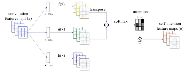
Summary of the Self-Attention Module Used in the Self-Attention GAN.
Taken from: Self-Attention Generative Adversarial Networks.
Additionally, the model is trained via hinge loss, commonly used for training support vector machines.
In SAGAN, the proposed attention module has been applied to both generator and discriminator, which are trained in an alternating fashion by minimizing the hinge version of the adversarial loss
— Self-Attention Generative Adversarial Networks, 2018.
The BigGAN uses the model architecture with attention modules from SAGAN and is trained via hinge loss.
Appendix B of the paper titled “Architectural Details” provides a summary of the modules and their configurations used in the generator and discriminator models. There are two versions of the model described BigGAN and BigGAN-deep, the latter involving deeper resnet modules and, in turn, achieving better results.
2. Class Conditional Information
The class information is provided to the generator model via class-conditional batch normalization.
This was described by Vincent Dumoulin, et al. in their 2016 paper titled “A Learned Representation For Artistic Style.” In the paper, the technique is referred to as “conditional instance normalization” that involves normalizing activations based on the statistics from images of a given style, or in the case of BigGAN, images of a given class.
We call this approach conditional instance normalization. The goal of the procedure is [to] transform a layer’s activations x into a normalized activation z specific to painting style s.
— A Learned Representation For Artistic Style, 2016.
Class information is provided to the discriminator via projection.
This is described by Takeru Miyato, et al. in their 2018 paper titled “Spectral Normalization for Generative Adversarial Networks.” This involves using an integer embedding of the class value that is concatenated into an intermediate layer of the network.
Discriminator for conditional GANs. For computational ease, we embedded the integer label y in {0, . . . , 1000} into 128 dimension before concatenating the vector to the output of the intermediate layer.
— Spectral Normalization for Generative Adversarial Networks, 2018.
Instead of using one class embedding per class label, a shared embedding was used in order to reduce the number of weights.
Instead of having a separate layer for each embedding, we opt to use a shared embedding, which is linearly projected to each layer’s gains and biases. This reduces computation and memory costs, and improves training speed (in number of iterations required to reach a given performance) by 37%.
— Large Scale GAN Training for High Fidelity Natural Image Synthesis, 2018.
3. Spectral Normalization
The weights of the generator are normalized using spectral normalization.
Spectral normalization for use in GANs was described by Takeru Miyato, et al. in their 2018 paper titled “Spectral Normalization for Generative Adversarial Networks.” Specifically, it involves normalizing the spectral norm of the weight matrix.
Our spectral normalization normalizes the spectral norm of the weight matrix W so that it satisfies the Lipschitz constraint sigma(W) = 1:
— Spectral Normalization for Generative Adversarial Networks, 2018.
The efficient implementation requires a change to the weight updates during mini-batch stochastic gradient descent, described in Appendix A of the spectral normalization paper.
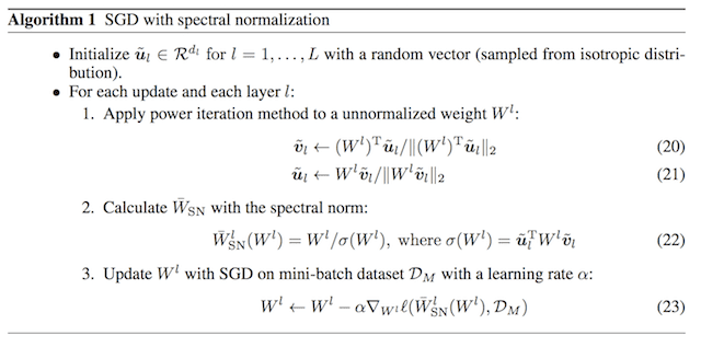
Algorithm for SGD With Spectral Normalization
Taken from: Spectral Normalization for Generative Adversarial Networks
4. Update Discriminator More Than Generator
In the GAN training algorithm, it is common to first update the discriminator model and then to update the generator model.
The BigGAN slightly modifies this and updates the discriminator model twice before updating the generator model in each training iteration.
5. Moving Average of Model Weights
The generator model is evaluated based on the images that are generated.
Before images are generated for evaluation, the model weights are averaged across prior training iterations using a moving average.
This approach to model weight moving average for generator evaluation was described and used by Tero Karras, et al. in their 2017 paper titled “Progressive Growing of GANs for Improved Quality, Stability, and Variation.”
… for visualizing generator output at any given point during the training, we use an exponential running average for the weights of the generator with decay 0.999.
— Progressive Growing of GANs for Improved Quality, Stability, and Variation, 2017.
6. Orthogonal Weight Initialization
Model weights are initialized using Orthogonal Initialization.
This was described by Andrew Saxe, et al. in their 2013 paper titled “Exact Solutions To The Nonlinear Dynamics Of Learning In Deep Linear Neural Networks.” This involves setting the weights to be a random orthogonal matrix.
… the initial weights in each layer to be a random orthogonal matrix (satisfying W^T . W = I) …
— Exact Solutions To The Nonlinear Dynamics Of Learning In Deep Linear Neural Networks, 2013.
Note that Keras supports orthogonal weight initialization directly.
7. Larger Batch Size
Very large batch sizes were tested and evaluated.
This includes batch sizes of 256, 512, 1024, and 2,048 images.
Larger batch sizes generally resulted in better quality images, with the best image quality achieved with a batch size of 2,048 images.
… simply increasing the batch size by a factor of 8 improves the state-of-the-art IS by 46%.
— Large Scale GAN Training for High Fidelity Natural Image Synthesis, 2018.
The intuition is that the larger batch size provides more “modes”, and in turn, provides better gradient information for updating the models.
We conjecture that this is a result of each batch covering more modes, providing better gradients for both networks.
— Large Scale GAN Training for High Fidelity Natural Image Synthesis, 2018.
8. More Model Parameters
The number of model parameters was also dramatically increased.
This was achieved by doubling the number of channels or feature maps (filters) in each layer.
We then increase the width (number of channels) in each layer by 50%, approximately doubling the number of parameters in both models. This leads to a further IS improvement of 21%, which we posit is due to the increased capacity of the model relative to the complexity of the dataset.
— Large Scale GAN Training for High Fidelity Natural Image Synthesis, 2018.
9. Skip-z Connections
Skip connections were added to the generator model to directly connect the input latent point to specific layers deep in the network.
These are referred to as skip-z connections, where z refers to the input latent vector.
Next, we add direct skip connections (skip-z) from the noise vector z to multiple layers of G rather than just the initial layer. The intuition behind this design is to allow G to use the latent space to directly influence features at different resolutions and levels of hierarchy. […] Skip-z provides a modest performance improvement of around 4%, and improves training speed by a further 18%.
— Large Scale GAN Training for High Fidelity Natural Image Synthesis, 2018.
10. Truncation Trick
The truncation trick involves using a different distribution for the generator’s latent space during training than during inference or image synthesis.
A Gaussian distribution is used during training, and a truncated Gaussian is used during inference. This is referred to as the “truncation trick.”
We call this the Truncation Trick: truncating a z vector by resampling the values with magnitude above a chosen threshold leads to improvement in individual sample quality at the cost of reduction in overall sample variety.
— Large Scale GAN Training for High Fidelity Natural Image Synthesis, 2018.
The truncation trick provides a trade-off between image quality or fidelity and image variety. A more narrow sampling range results in better quality, whereas a larger sampling range results in more variety in sampled images.
This technique allows fine-grained, post-hoc selection of the trade-off between sample quality and variety for a given G.
— Large Scale GAN Training for High Fidelity Natural Image Synthesis, 2018.
11. Orthogonal Regularization
Not all models respond well to the truncation trick.
Some of the deeper models would provide saturated artifacts when the truncation trick was used.
To better encourage a broader range of models to work well with the truncation trick, orthogonal regularization was used.
This was introduced by Andrew Brock, et al. in their 2016 paper titled “Neural Photo Editing with Introspective Adversarial Networks.”
This is related to the orthogonal weight initialization and introduces a weight regularization term to encourage the weights to maintain their orthogonal property.
Orthogonality is a desirable quality in ConvNet filters, partially because multiplication by an orthogonal matrix leaves the norm of the original matrix unchanged. […] we propose a simple weight regularization technique, Orthogonal Regularization, that encourages weights to be orthogonal by pushing them towards the nearest orthogonal manifold.
— Neural Photo Editing with Introspective Adversarial Networks, 2016.
Example of Images Generated by BigGAN
The BigGAN is capable of generating large, high-quality images.
In this section, we will review a few examples presented in the paper.
Below are some examples of high-quality images generated by BigGAN.

Examples of High-Quality Class-Conditional Images Generated by BigGAN.
Taken from: Large Scale GAN Training for High Fidelity Natural Image Synthesis.
Below are examples of large and high-quality images generated by BigGAN.
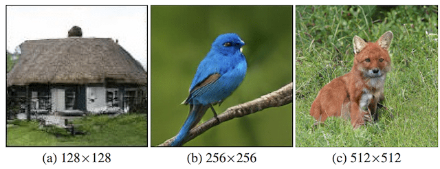
Examples of Large High-Quality Class-Conditional Images Generated by BigGAN.
Taken from: Large Scale GAN Training for High Fidelity Natural Image Synthesis.
One of the issues described when training BigGAN generators is the idea of “class leakage”, a new type of failure mode.
Below is an example of class leakage from a partially trained BigGAN, showing a cross between a tennis ball and perhaps a dog.

Examples of Class Leakage in an Image Generated by Partially Trained BigGAN.
Taken from: Large Scale GAN Training for High Fidelity Natural Image Synthesis.
Below are some additional images generated by the BigGAN at 256×256 resolution.

Examples of Large High-Quality 256×256 Class-Conditional Images Generated by BigGAN.
Taken from: Large Scale GAN Training for High Fidelity Natural Image Synthesis.
Below are some more images generated by the BigGAN at 512×512 resolution.
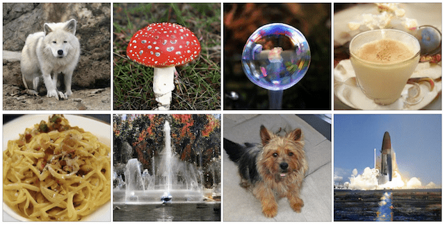
Examples of Large High-Quality 512×512 Class-Conditional Images Generated by BigGAN.
Taken from: Large Scale GAN Training for High Fidelity Natural Image Synthesis.
Further Reading
This section provides more resources on the topic if you are looking to go deeper.
Papers
- Large Scale GAN Training for High Fidelity Natural Image Synthesis, 2018.
- Large Scale GAN Training for High Fidelity Natural Image Synthesis, ICLR 2019.
- Self-Attention Generative Adversarial Networks, 2018.
- A Learned Representation For Artistic Style, 2016.
- Spectral Normalization for Generative Adversarial Networks, 2018.
- Progressive Growing of GANs for Improved Quality, Stability, and Variation, 2017.
- Exact Solutions To The Nonlinear Dynamics Of Learning In Deep Linear Neural Networks, 2013.
- Neural Photo Editing with Introspective Adversarial Networks, 2016.
Code
Articles
Summary
In this post, you discovered the BigGAN model for scaling up class-conditional image synthesis.
Specifically, you learned:
- Image size and training brittleness remain large problems for GANs.
- Scaling up model size and batch size can result in dramatically larger and higher-quality images.
- Specific model architectural and training configurations required to scale up GANs.
Do you have any questions?
Ask your questions in the comments below and I will do my best to answer.



can you provide the keras implementation of big gan
Thanks for the suggestion.
Hi Jason,
Would be have, sometime, any GAN arquitecture with similar power to this one, to train on real sensor data in order to generate fake multivariate timeseries (e.g. 200 time steps x 8 variables) rather than images? Do you know any GAN or implementation capable of that?
Thank you
Best
Sorry, I don’t have examples of GANs for time series.
Thanks for the explanation.. Do you have any keras example to share which perform Self-Attention Module and Hinge Loss?
You’re welcome.
Not at this stage.
The information in Section 2, class conditional information, is misleading. With respect to conditioning for the discriminator, the BigGAN paper cites Miyato 2018, “cGANS with Projection Discriminator”, not the spectral normalization paper. Conditioning information is provided via projection, not concatenation.
Thanks.
Hi Jason,
So when using the hinge loss, as used in Miyatos 2018 paper “cGANS with Projection Discriminator”, would we expect the discriminator and generator loss to be minimized? i’m working on an example and it looks like the generators loss is increasing for the better performing models, so I’m a bit confused.
I’m not sure off the cuff re that paper. Generally with GANs, no, they don’t minimize loss/converge.
Thank you for this awesome explanations. How can I evaluate the BigGAN discriminator in unsupervised/unconditional Learning? and How the loss function should look like?
Hi!
I’m beginner in this domain and I hope that you will answer me. As we know the inputs of Generator and Discriminator are distributions. My question is how the images turn into distributions
Hi raga…the following resources may add clarity:
https://github.com/abhijitramesh/GAN-under-the-hood
https://towardsdatascience.com/how-gans-really-work-2e1db1f407bb
this is good
Thank you for your feedback! Let us know if we can help answer any questions regarding our tutorials or other content.