The Pix2Pix Generative Adversarial Network, or GAN, is an approach to training a deep convolutional neural network for image-to-image translation tasks.
The careful configuration of architecture as a type of image-conditional GAN allows for both the generation of large images compared to prior GAN models (e.g. such as 256×256 pixels) and the capability of performing well on a variety of different image-to-image translation tasks.
In this tutorial, you will discover how to develop a Pix2Pix generative adversarial network for image-to-image translation.
After completing this tutorial, you will know:
How to load and prepare the satellite image to Google maps image-to-image translation dataset.
How to develop a Pix2Pix model for translating satellite photographs to Google map images.
How to use the final Pix2Pix generator model to translate ad hoc satellite images.
The GAN architecture is comprised of a generator model for outputting new plausible synthetic images, and a discriminator model that classifies images as real (from the dataset) or fake (generated). The discriminator model is updated directly, whereas the generator model is updated via the discriminator model. As such, the two models are trained simultaneously in an adversarial process where the generator seeks to better fool the discriminator and the discriminator seeks to better identify the counterfeit images.
The Pix2Pix model is a type of conditional GAN, or cGAN, where the generation of the output image is conditional on an input, in this case, a source image. The discriminator is provided both with a source image and the target image and must determine whether the target is a plausible transformation of the source image.
The generator is trained via adversarial loss, which encourages the generator to generate plausible images in the target domain. The generator is also updated via L1 loss measured between the generated image and the expected output image. This additional loss encourages the generator model to create plausible translations of the source image.
The Pix2Pix GAN has been demonstrated on a range of image-to-image translation tasks such as converting maps to satellite photographs, black and white photographs to color, and sketches of products to product photographs.
Now that we are familiar with the Pix2Pix GAN, let’s prepare a dataset that we can use with image-to-image translation.
Want to Develop GANs from Scratch?
Take my free 7-day email crash course now (with sample code).
Click to sign-up and also get a free PDF Ebook version of the course.
Satellite to Map Image Translation Dataset
In this tutorial, we will use the so-called “maps” dataset used in the Pix2Pix paper.
This is a dataset comprised of satellite images of New York and their corresponding Google maps pages. The image translation problem involves converting satellite photos to Google maps format, or the reverse, Google maps images to Satellite photos.
The dataset is provided on the pix2pix website and can be downloaded as a 255-megabyte zip file.
Download the dataset and unzip it into your current working directory. This will create a directory called “maps” with the following structure:
1
2
3
maps
├── train
└── val
The train folder contains 1,097 images, whereas the validation dataset contains 1,099 images.
Images have a digit filename and are in JPEG format. Each image is 1,200 pixels wide and 600 pixels tall and contains both the satellite image on the left and the Google maps image on the right.
Sample Image From the Maps Dataset Including Both Satellite and Google Maps Image.
We can prepare this dataset for training a Pix2Pix GAN model in Keras. We will just work with the images in the training dataset. Each image will be loaded, rescaled, and split into the satellite and Google map elements. The result will be 1,097 color image pairs with the width and height of 256×256 pixels.
The load_images() function below implements this. It enumerates the list of images in a given directory, loads each with the target size of 256×512 pixels, splits each image into satellite and map elements and returns an array of each.
1
2
3
4
5
6
7
8
9
10
11
12
13
14
# load all images in a directory into memory
def load_images(path,size=(256,512)):
src_list,tar_list=list(),list()
# enumerate filenames in directory, assume all are images
forfilename inlistdir(path):
# load and resize the image
pixels=load_img(path+filename,target_size=size)
# convert to numpy array
pixels=img_to_array(pixels)
# split into satellite and map
sat_img,map_img=pixels[:,:256],pixels[:,256:]
src_list.append(sat_img)
tar_list.append(map_img)
return[asarray(src_list),asarray(tar_list)]
We can call this function with the path to the training dataset. Once loaded, we can save the prepared arrays to a new file in compressed format for later use.
The complete example is listed below.
1
2
3
4
5
6
7
8
9
10
11
12
13
14
15
16
17
18
19
20
21
22
23
24
25
26
27
28
29
30
31
32
# load, split and scale the maps dataset ready for training
from os import listdir
from numpy import asarray
from numpy import vstack
from keras.preprocessing.image import img_to_array
from keras.preprocessing.image import load_img
from numpy import savez_compressed
# load all images in a directory into memory
def load_images(path,size=(256,512)):
src_list,tar_list=list(),list()
# enumerate filenames in directory, assume all are images
Running the example loads all images in the training dataset, summarizes their shape to ensure the images were loaded correctly, then saves the arrays to a new file called maps_256.npz in compressed NumPy array format.
1
2
Loaded: (1096, 256, 256, 3) (1096, 256, 256, 3)
Saved dataset: maps_256.npz
This file can be loaded later via the load() NumPy function and retrieving each array in turn.
We can then plot some images pairs to confirm the data has been handled correctly.
Running this example loads the prepared dataset and summarizes the shape of each array, confirming our expectations of a little over one thousand 256×256 image pairs.
1
Loaded: (1096, 256, 256, 3) (1096, 256, 256, 3)
A plot of three image pairs is also created showing the satellite images on the top and Google map images on the bottom.
We can see that satellite images are quite complex and that although the Google map images are much simpler, they have color codings for things like major roads, water, and parks.
Plot of Three Image Pairs Showing Satellite Images (top) and Google Map Images (bottom).
Now that we have prepared the dataset for image translation, we can develop our Pix2Pix GAN model.
How to Develop and Train a Pix2Pix Model
In this section, we will develop the Pix2Pix model for translating satellite photos to Google maps images.
The same model architecture and configuration described in the paper was used across a range of image translation tasks. This architecture is both described in the body of the paper, with additional detail in the appendix of the paper, and a fully working implementation provided as open source with the Torch deep learning framework.
The implementation in this section will use the Keras deep learning framework based directly on the model described in the paper and implemented in the author’s code base, designed to take and generate color images with the size 256×256 pixels.
The architecture is comprised of two models: the discriminator and the generator.
The discriminator is a deep convolutional neural network that performs image classification. Specifically, conditional-image classification. It takes both the source image (e.g. satellite photo) and the target image (e.g. Google maps image) as input and predicts the likelihood of whether target image is real or a fake translation of the source image.
The discriminator design is based on the effective receptive field of the model, which defines the relationship between one output of the model to the number of pixels in the input image. This is called a PatchGAN model and is carefully designed so that each output prediction of the model maps to a 70×70 square or patch of the input image. The benefit of this approach is that the same model can be applied to input images of different sizes, e.g. larger or smaller than 256×256 pixels.
The output of the model depends on the size of the input image but may be one value or a square activation map of values. Each value is a probability for the likelihood that a patch in the input image is real. These values can be averaged to give an overall likelihood or classification score if needed.
The define_discriminator() function below implements the 70×70 PatchGAN discriminator model as per the design of the model in the paper. The model takes two input images that are concatenated together and predicts a patch output of predictions. The model is optimized using binary cross entropy, and a weighting is used so that updates to the model have half (0.5) the usual effect. The authors of Pix2Pix recommend this weighting of model updates to slow down changes to the discriminator, relative to the generator model during training.
The generator model is more complex than the discriminator model.
The generator is an encoder-decoder model using a U-Net architecture. The model takes a source image (e.g. satellite photo) and generates a target image (e.g. Google maps image). It does this by first downsampling or encoding the input image down to a bottleneck layer, then upsampling or decoding the bottleneck representation to the size of the output image. The U-Net architecture means that skip-connections are added between the encoding layers and the corresponding decoding layers, forming a U-shape.
The image below makes the skip-connections clear, showing how the first layer of the encoder is connected to the last layer of the decoder, and so on.
Architecture of the U-Net Generator Model Taken from Image-to-Image Translation With Conditional Adversarial Networks
The encoder and decoder of the generator are comprised of standardized blocks of convolutional, batch normalization, dropout, and activation layers. This standardization means that we can develop helper functions to create each block of layers and call it repeatedly to build-up the encoder and decoder parts of the model.
The define_generator() function below implements the U-Net encoder-decoder generator model. It uses the define_encoder_block() helper function to create blocks of layers for the encoder and the decoder_block() function to create blocks of layers for the decoder. The tanh activation function is used in the output layer, meaning that pixel values in the generated image will be in the range [-1,1].
The discriminator model is trained directly on real and generated images, whereas the generator model is not.
Instead, the generator model is trained via the discriminator model. It is updated to minimize the loss predicted by the discriminator for generated images marked as “real.” As such, it is encouraged to generate more real images. The generator is also updated to minimize the L1 loss or mean absolute error between the generated image and the target image.
The generator is updated via a weighted sum of both the adversarial loss and the L1 loss, where the authors of the model recommend a weighting of 100 to 1 in favor of the L1 loss. This is to encourage the generator strongly toward generating plausible translations of the input image, and not just plausible images in the target domain.
This can be achieved by defining a new logical model comprised of the weights in the existing standalone generator and discriminator model. This logical or composite model involves stacking the generator on top of the discriminator. A source image is provided as input to the generator and to the discriminator, although the output of the generator is connected to the discriminator as the corresponding “target” image. The discriminator then predicts the likelihood that the generator was a real translation of the source image.
The discriminator is updated in a standalone manner, so the weights are reused in this composite model but are marked as not trainable. The composite model is updated with two targets, one indicating that the generated images were real (cross entropy loss), forcing large weight updates in the generator toward generating more realistic images, and the executed real translation of the image, which is compared against the output of the generator model (L1 loss).
The define_gan() function below implements this, taking the already-defined generator and discriminator models as arguments and using the Keras functional API to connect them together into a composite model. Both loss functions are specified for the two outputs of the model and the weights used for each are specified in the loss_weights argument to the compile() function.
1
2
3
4
5
6
7
8
9
10
11
12
13
14
15
16
17
18
# define the combined generator and discriminator model, for updating the generator
def define_gan(g_model,d_model,image_shape):
# make weights in the discriminator not trainable
forlayer ind_model.layers:
ifnotisinstance(layer,BatchNormalization):
layer.trainable=False
# define the source image
in_src=Input(shape=image_shape)
# connect the source image to the generator input
gen_out=g_model(in_src)
# connect the source input and generator output to the discriminator input
dis_out=d_model([in_src,gen_out])
# src image as input, generated image and classification output
Next, we can load our paired images dataset in compressed NumPy array format.
This will return a list of two NumPy arrays: the first for source images and the second for corresponding target images.
1
2
3
4
5
6
7
8
9
10
# load and prepare training images
def load_real_samples(filename):
# load compressed arrays
data=load(filename)
# unpack arrays
X1,X2=data['arr_0'],data['arr_1']
# scale from [0,255] to [-1,1]
X1=(X1-127.5)/127.5
X2=(X2-127.5)/127.5
return[X1,X2]
Training the discriminator will require batches of real and fake images.
The generate_real_samples() function below will prepare a batch of random pairs of images from the training dataset, and the corresponding discriminator label of class=1 to indicate they are real.
1
2
3
4
5
6
7
8
9
10
11
# select a batch of random samples, returns images and target
The generate_fake_samples() function below uses the generator model and a batch of real source images to generate an equivalent batch of target images for the discriminator.
These are returned with the label class-0 to indicate to the discriminator that they are fake.
1
2
3
4
5
6
7
# generate a batch of images, returns images and targets
Typically, GAN models do not converge; instead, an equilibrium is found between the generator and discriminator models. As such, we cannot easily judge when training should stop. Therefore, we can save the model and use it to generate sample image-to-image translations periodically during training, such as every 10 training epochs.
We can then review the generated images at the end of training and use the image quality to choose a final model.
The summarize_performance() function implements this, taking the generator model at a point during training and using it to generate a number, in this case three, of translations of randomly selected images in the dataset. The source, generated image, and expected target are then plotted as three rows of images and the plot saved to file. Additionally, the model is saved to an H5 formatted file that makes it easier to load later.
Both the image and model filenames include the training iteration number, allowing us to easily tell them apart at the end of training.
1
2
3
4
5
6
7
8
9
10
11
12
13
14
15
16
17
18
19
20
21
22
23
24
25
26
27
28
29
30
31
32
33
# generate samples and save as a plot and save the model
Finally, we can train the generator and discriminator models.
The train() function below implements this, taking the defined generator, discriminator, composite model, and loaded dataset as input. The number of epochs is set at 100 to keep training times down, although 200 was used in the paper. A batch size of 1 is used as is recommended in the paper.
Training involves a fixed number of training iterations. There are 1,097 images in the training dataset. One epoch is one iteration through this number of examples, with a batch size of one means 1,097 training steps. The generator is saved and evaluated every 10 epochs or every 10,970 training steps, and the model will run for 100 epochs, or a total of 109,700 training steps.
Each training step involves first selecting a batch of real examples, then using the generator to generate a batch of matching fake samples using the real source images. The discriminator is then updated with the batch of real images and then fake images.
Next, the generator model is updated providing the real source images as input and providing class labels of 1 (real) and the real target images as the expected outputs of the model required for calculating loss. The generator has two loss scores as well as the weighted sum score returned from the call to train_on_batch(). We are only interested in the weighted sum score (the first value returned) as it is used to update the model weights.
Finally, the loss for each update is reported to the console each training iteration and model performance is evaluated every 10 training epochs.
The example might take about two hours to run on modern GPU hardware.
Note: Your results may vary given the stochastic nature of the algorithm or evaluation procedure, or differences in numerical precision. Consider running the example a few times and compare the average outcome.
The loss is reported each training iteration, including the discriminator loss on real examples (d1), discriminator loss on generated or fake examples (d2), and generator loss, which is a weighted average of adversarial and L1 loss (g).
If loss for the discriminator goes to zero and stays there for a long time, consider re-starting the training run as it is an example of a training failure.
1
2
3
4
5
6
7
8
9
10
11
12
>1, d1[0.566] d2[0.520] g[82.266]
>2, d1[0.469] d2[0.484] g[66.813]
>3, d1[0.428] d2[0.477] g[79.520]
>4, d1[0.362] d2[0.405] g[78.143]
>5, d1[0.416] d2[0.406] g[72.452]
...
>109596, d1[0.303] d2[0.006] g[5.792]
>109597, d1[0.001] d2[1.127] g[14.343]
>109598, d1[0.000] d2[0.381] g[11.851]
>109599, d1[1.289] d2[0.547] g[6.901]
>109600, d1[0.437] d2[0.005] g[10.460]
>Saved: plot_109600.png and model_109600.h5
Models are saved every 10 epochs and saved to a file with the training iteration number. Additionally, images are generated every 10 epochs and compared to the expected target images. These plots can be assessed at the end of the run and used to select a final generator model based on generated image quality.
At the end of the run, will you will have 10 saved model files and 10 plots of generated images.
After the first 10 epochs, map images are generated that look plausible, although the lines for streets are not entirely straight and images contain some blurring. Nevertheless, large structures are in the right places with mostly the right colors.
Plot of Satellite to Google Map Translated Images Using Pix2Pix After 10 Training Epochs
Generated images after about 50 training epochs begin to look very realistic, at least to mean, and quality appears to remain good for the remainder of the training process.
Note the first generated image example below (right column, middle row) that includes more useful detail than the real Google map image.
Plot of Satellite to Google Map Translated Images Using Pix2Pix After 100 Training Epochs
Now that we have developed and trained the Pix2Pix model, we can explore how they can be used in a standalone manner.
How to Translate Images With a Pix2Pix Model
Training the Pix2Pix model results in many saved models and samples of generated images for each.
More training epochs does not necessarily mean a better quality model. Therefore, we can choose a model based on the quality of the generated images and use it to perform ad hoc image-to-image translation.
In this case, we will use the model saved at the end of the run, e.g. after 100 epochs or 109,600 training iterations.
A good starting point is to load the model and use it to make ad hoc translations of source images in the training dataset.
First, we can load the training dataset. We can use the same function named load_real_samples() for loading the dataset as was used when training the model.
1
2
3
4
5
6
7
8
9
10
# load and prepare training images
def load_real_samples(filename):
# load compressed ararys
data=load(filename)
# unpack arrays
X1,X2=data['arr_0'],data['arr_1']
# scale from [0,255] to [-1,1]
X1=(X1-127.5)/127.5
X2=(X2-127.5)/127.5
return[X1,X2]
This function can be called as follows:
1
2
3
4
...
# load dataset
[X1,X2]=load_real_samples('maps_256.npz')
print('Loaded',X1.shape,X2.shape)
Next, we can load the saved Keras model.
1
2
3
...
# load model
model=load_model('model_109600.h5')
Next, we can choose a random image pair from the training dataset to use as an example.
1
2
3
4
...
# select random example
ix=randint(0,len(X1),1)
src_image,tar_image=X1[ix],X2[ix]
We can provide the source satellite image as input to the model and use it to predict a Google map image.
1
2
3
...
# generate image from source
gen_image=model.predict(src_image)
Finally, we can plot the source, generated image, and the expected target image.
The plot_images() function below implements this, providing a nice title above each image.
1
2
3
4
5
6
7
8
9
10
11
12
13
14
15
16
17
# plot source, generated and target images
def plot_images(src_img,gen_img,tar_img):
images=vstack((src_img,gen_img,tar_img))
# scale from [-1,1] to [0,1]
images=(images+1)/2.0
titles=['Source','Generated','Expected']
# plot images row by row
foriinrange(len(images)):
# define subplot
pyplot.subplot(1,3,1+i)
# turn off axis
pyplot.axis('off')
# plot raw pixel data
pyplot.imshow(images[i])
# show title
pyplot.title(titles[i])
pyplot.show()
This function can be called with each of our source, generated, and target images.
1
2
3
...
# plot all three images
plot_images(src_image,gen_image,tar_image)
Tying all of this together, the complete example of performing an ad hoc image-to-image translation with an example from the training dataset is listed below.
1
2
3
4
5
6
7
8
9
10
11
12
13
14
15
16
17
18
19
20
21
22
23
24
25
26
27
28
29
30
31
32
33
34
35
36
37
38
39
40
41
42
43
44
45
46
47
48
# example of loading a pix2pix model and using it for image to image translation
from keras.models import load_model
from numpy import load
from numpy import vstack
from matplotlib import pyplot
from numpy.random import randint
# load and prepare training images
def load_real_samples(filename):
# load compressed arrays
data=load(filename)
# unpack arrays
X1,X2=data['arr_0'],data['arr_1']
# scale from [0,255] to [-1,1]
X1=(X1-127.5)/127.5
X2=(X2-127.5)/127.5
return[X1,X2]
# plot source, generated and target images
def plot_images(src_img,gen_img,tar_img):
images=vstack((src_img,gen_img,tar_img))
# scale from [-1,1] to [0,1]
images=(images+1)/2.0
titles=['Source','Generated','Expected']
# plot images row by row
foriinrange(len(images)):
# define subplot
pyplot.subplot(1,3,1+i)
# turn off axis
pyplot.axis('off')
# plot raw pixel data
pyplot.imshow(images[i])
# show title
pyplot.title(titles[i])
pyplot.show()
# load dataset
[X1,X2]=load_real_samples('maps_256.npz')
print('Loaded',X1.shape,X2.shape)
# load model
model=load_model('model_109600.h5')
# select random example
ix=randint(0,len(X1),1)
src_image,tar_image=X1[ix],X2[ix]
# generate image from source
gen_image=model.predict(src_image)
# plot all three images
plot_images(src_image,gen_image,tar_image)
Running the example will select a random image from the training dataset, translate it to a Google map, and plot the result compared to the expected image.
Note: Your results may vary given the stochastic nature of the algorithm or evaluation procedure, or differences in numerical precision. Consider running the example a few times and compare the average outcome.
In this case, we can see that the generated image captures large roads with orange and yellow as well as green park areas. The generated image is not perfect but is very close to the expected image.
Plot of Satellite to Google Map Image Translation With Final Pix2Pix GAN Model
We may also want to use the model to translate a given standalone image.
We can select an image from the validation dataset under maps/val and crop the satellite element of the image. This can then be saved and used as input to the model.
In this case, we will use “maps/val/1.jpg“.
Example Image From the Validation Part of the Maps Dataset
We can use an image program to create a rough crop of the satellite element of this image to use as input and save the file as satellite.jpg in the current working directory.
Example of a Cropped Satellite Image to Use as Input to the Pix2Pix Model.
We must load the image as a NumPy array of pixels with the size of 256×256, rescale the pixel values to the range [-1,1], and then expand the single image dimensions to represent one input sample.
The load_image() function below implements this, returning image pixels that can be provided directly to a loaded Pix2Pix model.
1
2
3
4
5
6
7
8
9
10
11
# load an image
def load_image(filename,size=(256,256)):
# load image with the preferred size
pixels=load_img(filename,target_size=size)
# convert to numpy array
pixels=img_to_array(pixels)
# scale from [0,255] to [-1,1]
pixels=(pixels-127.5)/127.5
# reshape to 1 sample
pixels=expand_dims(pixels,0)
returnpixels
We can then load our cropped satellite image.
1
2
3
4
...
# load source image
src_image=load_image('satellite.jpg')
print('Loaded',src_image.shape)
As before, we can load our saved Pix2Pix generator model and generate a translation of the loaded image.
1
2
3
4
5
...
# load model
model=load_model('model_109600.h5')
# generate image from source
gen_image=model.predict(src_image)
Finally, we can scale the pixel values back to the range [0,1] and plot the result.
1
2
3
4
5
6
7
...
# scale from [-1,1] to [0,1]
gen_image=(gen_image+1)/2.0
# plot the image
pyplot.imshow(gen_image[0])
pyplot.axis('off')
pyplot.show()
Tying this all together, the complete example of performing an ad hoc image translation with a single image file is listed below.
1
2
3
4
5
6
7
8
9
10
11
12
13
14
15
16
17
18
19
20
21
22
23
24
25
26
27
28
29
30
31
32
33
# example of loading a pix2pix model and using it for one-off image translation
from keras.models import load_model
from keras.preprocessing.image import img_to_array
from keras.preprocessing.image import load_img
from numpy import load
from numpy import expand_dims
from matplotlib import pyplot
# load an image
def load_image(filename,size=(256,256)):
# load image with the preferred size
pixels=load_img(filename,target_size=size)
# convert to numpy array
pixels=img_to_array(pixels)
# scale from [0,255] to [-1,1]
pixels=(pixels-127.5)/127.5
# reshape to 1 sample
pixels=expand_dims(pixels,0)
returnpixels
# load source image
src_image=load_image('satellite.jpg')
print('Loaded',src_image.shape)
# load model
model=load_model('model_109600.h5')
# generate image from source
gen_image=model.predict(src_image)
# scale from [-1,1] to [0,1]
gen_image=(gen_image+1)/2.0
# plot the image
pyplot.imshow(gen_image[0])
pyplot.axis('off')
pyplot.show()
Running the example loads the image from file, creates a translation of it, and plots the result.
The generated image appears to be a reasonable translation of the source image.
The streets do not appear to be straight lines and the detail of the buildings is a bit lacking. Perhaps with further training or choice of a different model, higher-quality images could be generated.
Plot of Satellite Image Translated to Google Maps With Final Pix2Pix GAN Model
How to Translate Google Maps to Satellite Images
Now that we are familiar with how to develop and use a Pix2Pix model for translating satellite images to Google maps, we can also explore the reverse.
That is, we can develop a Pix2Pix model to translate Google map images to plausible satellite images. This requires that the model invent or hallucinate plausible buildings, roads, parks, and more.
We can use the same code to train the model with one small difference. We can change the order of the datasets returned from the load_real_samples() function; for example:
1
2
3
4
5
6
7
8
9
10
11
# load and prepare training images
def load_real_samples(filename):
# load compressed arrays
data=load(filename)
# unpack arrays
X1,X2=data['arr_0'],data['arr_1']
# scale from [0,255] to [-1,1]
X1=(X1-127.5)/127.5
X2=(X2-127.5)/127.5
# return in reverse order
return[X2,X1]
Note: the order of X1 and X2 is reversed.
This means that the model will take Google map images as input and learn to generate satellite images.
Run the example as before.
Note: Your results may vary given the stochastic nature of the algorithm or evaluation procedure, or differences in numerical precision. Consider running the example a few times and compare the average outcome.
As before, the loss of the model is reported each training iteration. If loss for the discriminator goes to zero and stays there for a long time, consider re-starting the training run as it is an example of a training failure.
1
2
3
4
5
6
7
8
9
10
11
12
>1, d1[0.442] d2[0.650] g[49.790]
>2, d1[0.317] d2[0.478] g[56.476]
>3, d1[0.376] d2[0.450] g[48.114]
>4, d1[0.396] d2[0.406] g[62.903]
>5, d1[0.496] d2[0.460] g[40.650]
...
>109596, d1[0.311] d2[0.057] g[25.376]
>109597, d1[0.028] d2[0.070] g[16.618]
>109598, d1[0.007] d2[0.208] g[18.139]
>109599, d1[0.358] d2[0.076] g[22.494]
>109600, d1[0.279] d2[0.049] g[9.941]
>Saved: plot_109600.png and model_109600.h5
It is harder to judge the quality of generated satellite images, nevertheless, plausible images are generated after just 10 epochs.
Plot of Google Map to Satellite Translated Images Using Pix2Pix After 10 Training Epochs
As before, image quality will improve and will continue to vary over the training process. A final model can be chosen based on generated image quality, not total training epochs.
The model appears to have little difficulty in generating reasonable water, parks, roads, and more.
Plot of Google Map to Satellite Translated Images Using Pix2Pix After 90 Training Epochs
Extensions
This section lists some ideas for extending the tutorial that you may wish to explore.
Standalone Satellite. Develop an example of translating standalone Google map images to satellite images, as we did for satellite to Google map images.
New Image. Locate a satellite image for an entirely new location and translate it to a Google map and consider the result compared to the actual image in Google maps.
More Training. Continue training the model for another 100 epochs and evaluate whether the additional training results in further improvements in image quality.
Image Augmentation. Use some minor image augmentation during training as described in the Pix2Pix paper and evaluate whether it results in better quality generated images.
If you explore any of these extensions, I’d love to know.
Post your findings in the comments below.
Further Reading
This section provides more resources on the topic if you are looking to go deeper.
From a digital signal processing viewpoint a weighted sum is an adjustable filter.
Each layer in a conventional artificial neural network has n of those filters and the total compute is a brutal n squared fused multiply accumulates.
A fast Fourier transform is a fixed (nonadjustable) bank of filters, where each filter picks out frequency/phase.
There are other transforms that act as filter banks too, such as the fast Walsh Hadamard transform and these often require far less compute (eg. nlog(n)) than a filter bank of weighed sums.
The question then is why not use an efficient transform based filter bank and adjust the nonlinear functions in a neural network by individually parameterizing them?
Ie. change what you adjust: https://github.com/S6Regen/Fixed-Filter-Bank-Neural-Networks https://discourse.numenta.org/t/fixed-filter-bank-neural-networks/6392 https://discourse.numenta.org/t/distributed-representations-1984-by-hinton/6378/10
It seems to me that the discriminator is not a 70×70 PatchGAN, since the 4th layer should not be there. With that layer it seems like the discirminator is a 142×142 PatchGAN. Please correct me if I am mistaken.
That example has the same structure, 6 layers of Conv2D (including the last one). But when looking at the beginning of the post where You are calculating the receptive field with 5 layers of Conv layers. The calculation also states that there are only 3 layers of Conv2D with a stride of 2. I believe that the layer named C512 should be the second to last layer.
Hi Jason, thanks for the great tutorials. I agreed with Villem that the current discriminator model is a 142×142 PatchGAN. For a 70x70PatchGAN, I think it should be only 3 layers with 4×4 kernel and 2×2 stride (remove the C512).
If anyone else has the same confusion with me, please let me know. thanks:)
Thanks for the tutorial.
My question is in original paper they are giving the direction as configurable parameter.
But in your implementation I am unable to see that one.
How can do that for both direction.
Please explain
Hello, thanks for the great article.
I have one question, but why you scale the image to [-1, 1] instead of [0, 1]?
Does this make the model behave differently?
Hi sir, is it possible to train this model with inputs and output of different sizes?
For example, I have 3 image a,b,c with size 50x50x3. I want the model to generate c from a,b. First I append a and b to get d with size 50x100x3, then use d as input, c as output
First of all, thank you very much for posting this tutorial, I learned a lot from it.
I have a question.
Do u think if I leave the picture resolution as it is rather than compressing them.
The performance is gonna be better? As my pictures between translation is very minor.
I am using a machine with 8 gpus (8 X p4000) 🙂
I mean, for example, while training on darknet, changing batch size directly affects gpu memory usage. But this codes use only 100 mb of each gpu. And batch size doesn’t affect it. So I need an adjustment just like on darknet so that I can use full capability of gpus.
Thanks
Swapping out the training data for the SEN1-2 dataset had amazing results. I can now translate Sentinel 1 images to RGB Sentinel 2! Many thanks for such a thorough tutorial.
Awesome tutorial on Pix2Pix. Your other GAN articles were great too and very helpful. After reading your tutorials, I was able to implement my own Pix2Pix project. All the code is on my GItHub. https://github.com/michaelnation26/pix2pix-edges-with-color
    tensorflow.python.framework.errors_impl.UnknownError:  Failed to get convolution algorithm. This is probably because cuDNN failed to initialize, so try looking to see if a warning log message was printed above.

             [[node conv2d_7/convolution (defined at C:\Users\ACSECKIN\Anaconda3\envs\tensorflow\lib\site-packages\tensorflow_core\python\framework\ops.py:1751) ]] [Op:__inference_keras_scratch_graph_4815]
Code works with CPU. But I want to run in the GPU to complete in less time. CPU time is about 16 hours. I am open to any alternative to decrease the training time.
Based on my experience, I receive this error message when my GPU does not have enough memory to handle the process. Maybe try reducing the computational workload by using a smaller image? If not, use CPU if you are fine with it.
Thought that more epochs give better results, since GAN`s cannot converge… so by theory no over fitting.. but I am new in the field, so I will look more into it 🙂
Thank you for your awesome post, it is really detailed and helpful! I have a question about normalizing between [0, 255] to [-1, 1]. My images are single channel and the maximum and minimum pixel values vary for each image, from 0 to around 3-4 (depends on the image). How should I go about normalizing the images? Should I take the maximum of the whole batch of samples and normalize, or should I take the maximum for each sample and normalize each individually?
Also, when translating new images, what would be the values of image? Would it be between -1 to 1? If yes, how should I “denormalize” the values to the original? Thank you for your help!
I recommend selecting a min and max that you expect to see for all time and use that to scale the data. If not known or it cannot be known, use the limits of the domain (e.g. 0 and 255).
Thank you for your suggestions! How would you suggest I “de-normalize” the data during testing? Should I use the same range (I am taking the range from the training data) and reverse the process on the test data?
Thank you very much for sharing such an in-depth analysis of Pix2Pix GAN. It is really helpful for early career researchers like me who don’t have a CS background. I thought of applying this fro solving and inverse problems in Digital Holographic Microscopy and I am now intrigued by the preliminary results I have got. As you know, the output of the model is a translated image, hence it is not possible to calculate the model accuracy. I am looking for an image quality metric such as SSIM. Do you have any suggestions?
Thank You,
PS: As this post helped me enormously, I would like to cite your works on GANs in the future.
Hi! Currently implementing this with images with shape (256, 512, 3) and keep running to an error as follows:
“ValueError: A target array with shape (1, 16, 16, 1) was passed for an output of shape (None, 16, 32, 1) while using as loss binary_crossentropy. This loss expects targets to have the same shape as the output.”
I assume that this is due to the downsampling? Any help would be appreciated
Thank you for this tutorial and simple code. I used it to perform image-to-image translation from Köppen–Geiger climate classification map ( https://en.wikipedia.org/wiki/K%C3%B6ppen_climate_classification ) to real satellite data, with truly amazing results, but I have a question.
In my strategy I create near one thousand pairs of 256×256 tiles from the Köppen–Geiger map (present in the Wikipedia article above), and a high-resolution satellite map of the Earth. In order to minimize deformation on tiles pairs near poles I use orthographic projection. This gives me nice pairs of image for GAN training (see https://photos.app.goo.gl/eGvpXghUtCB9kqkX6 ).
I trained the GAN until the end (n_epochs=100) with amazing results. Using training data give truly convincing satellite map validation (https://photos.app.goo.gl/a4EV6Gh15hAnYokm7). Even with hand-painted or with source image converted from a random image into Köppen–Geiger colormap, results are very nice (https://photos.app.goo.gl/eGbFmTH7YqYi4xfu5).
However I noticed that the result lacked of “relief” effect. Moreover, on large landmasses where the climate does not change but the topography noticeably affects the satellite view (e.g Tibetan Plateau or the Grand Canyon), the model results in “flat” satellite views.
As the climate map is composed of only 29 different indexed colors (plus the one I added for oceans), a simple label-to-image translation could be used, instead of using a full RGB climate image as input.
So my idea was to store a heightmap of the earth on the first channel of the input image, and the normalized indexed climate color on the second channel. The third channel is kept unused. It results in a Red-Green image where the Red channel is the heightmap and the Green channel is normalized climate index (see https://photos.app.goo.gl/cN1cmCNLSXwwqzNB9).
The problem is that training with this input images give bad results compared to my first try (only climate date). Results were already convincing after 30 epochs in my my first try, with smooth transition between climates, why here the boundaries are clearly visible in generated images (see https://photos.app.goo.gl/Q1vjjeY8ewWrCZYv5 ).
I tried to run the training several times to ensure that it was not purely bad luck, with the same result.
I don’t understand because climate index can clearly be stored on one channel without information loss, and heightmap provides additional data, so it should improve the results. Is it simply because it needs more epochs ?
Thank you in advance and sorry for the long post and for my english, it is not my native language.
Two thoughts off the cuff. One would be to make image synthesis conditional on two input images (source and the height map). A second would be to have 2 steps – one step to generate the initial translation and a second to improve the generated image with a height map.
Thank you very much ! The aim is to develop a tool for worlbuidling and create realistic maps of imaginary planets (following Atrifexian’s tutorials https://www.youtube.com/watch?v=5lCbxMZJ4zA&t=1s ).
I used the idea of using R and G channels for heightmap and climate following this thread concerning the pytorch implementation : https://github.com/junyanz/pytorch-CycleGAN-and-pix2pix/issues/498. They recommend to concatenate the input images, but it seems that your code is limited to 3 channels and as I’m a complete beginner I still don’t know how to use more than one image as input.
However it seems indeed that training on more epochs actually gives good results with my method. Maybe 100 is not enough, so I restarted it with a limit of 1000 epochs. However I have to redo the first 100, an I run the code on Google Colab which seems to be very unstable (I only managed to reach 100 epochs twice).
Do you have a tutorial on how to make complete checkpoints in order to continue the training in case of crash ? If I understand well, your summarize_performance function only save the generator model, so we should have to save the whole gan_model and reload it for later training. Do you have documentation or examples concerning this ?
Thank you so much for your tutorial. I’ll keep you informed on later developments !
Hello,
Thanks for the wonderful tutorial, Please how can I adapt the generator and the descriminator in order to make a transition from matrix (2,64) into matrix(2,64)
I have a dataset consisting of 216 images. I trained for 100 epochs but unfortunately the results are not good. Can you help me how can I improve the results?
This is probably a newbie question, but I am new to GANs. In my limited experience with deep CNNs, I used the validation data during the training process to sort of evaluate how well it was “learning”> I then had another dataset I called the “test” dataset that I used after the training process was complete. Here it seems like you don’t use any validation during the training process. And what you call validation is what I call the test dataset. Is that something unique to GANs or can validation be included in the training process?
Hi Jason,
From the theory, we understand that dicriminator learns the objective loss function.However referring to define_GAN(),line 56 in the code, I am not able to see the object loss learnt by discriminator getting passed to GAN model. I see that the model doesnot converge as expected
Thanks for the great tutorial. I need help with something. I want to see accuracy metrics for both train dataset and test dataset throughout the training process. And I want to see this for each epoch, not for each steps. Like a standart CNN model training procedure. How can add this things to code ? I couldn’t apply it because it is different than standard CNN codes. I would really appreciate it if you answer. Thank you.
Hi Jason,
Thanks for the great tutorial. I have a problem with image scales. In first step, after splitting the input images, I check the image size, instead of of 256*256 pixel they are 134*139 with background. Also, at translation a given standalone image using by model step, the output should be 256*256 same as input, but I get 252*262 output again with background.
I was wondering if you would mind letting me know where is the problem?
Thanks in advance
Ehsan
Great work Jason. Just one question: do you believe that this approach could work using a RGB satellite image against its mask image, to make some kind of image segmentation ?
Thanks in advance
You can add two ‘dummy’ layers to the mask image, so that it is compatible as a target image to the RGB source image. Your RGB image as numpy array will be in the shape of (nr images, width, height, nr bands) where nr bands is three. Your mask image will be in shape (nr images, width, height, nr bands) where nr bands is one. So if you add two bands to the mask image, with e.g. only -1 values, then they are compatible.
It is an interesting article publish here. I am new using this, i want some question for the first script for clear explanation :
1. I saw the loaded data is maps in train and test folder. I want to know which 3 sample was loaded from the folder train? because the results was : (1096, 256, 256, 3) (1096, 256, 256, 3). I understand 1096 is the certain amount of image in that folder. and 256 I still dont understand because when I open picture 256 is not the same as the it was loaded.
2. I saw the folder contain image in train and test. I want to ask the train, example 1.jpg it contains two image from satellite. May I know how to develop the left picture and the right picture or it develop itself? Also in test does it develop itself or have to save it first?
Need some explanation for preparing using it in the future. Thank you
thank you for replying. For my second question I saw the folder train and test contains an image. So the question come up :
1.Does the image build itself?
2. If No, how do you make the images side by side that contains two image in one image.
hi thank you for your work !
I need your help,I need the same model but the input of the generator is one channel and not three .
I have tried to change it but it does’nt work .thank you
hello I have this problem I dont know why :
ValueError: Graph disconnected: cannot obtain value for tensor Tensor(“input_14:0”, shape=(?, 256, 256, 3), dtype=float32) at layer “input_14”. The following previous layers were accessed without issue: [‘input_15’]
Hi. I tried to use a different dataset using this code. Specifically the edges2shoes dataset but i was not able to convert it into npz file. Everytime i ran into memory error. My ram is 16GB still that was not enough. I managed to create multiple npz files though. How should i proceed?
Also could you be kind enough to make tutorial of Tensorflow/Keras of pix2pixHD since it is much more accurate and better in side by side tests compared to normal pix2pix.
Hi Jason. Great Article. Good explanation. Your articles gave me a good overview and starting point when I started developing my own networks. But I have two questions:
1:) From what I can see the original code on Github seems to be slightly different to your code in this article when it comes to how you connect an encoder and a decoder layer. On Github data from an encoder layer passed to a decoder layer (via skip-connection) is unactivated, meaning that the data is passed directly after the convolution(or batch norm/dropout), in contrary to the solution here. Is this a mistake or variation ?
2.) What does the flag ‘training=True’ do when calling batch normalization layer or dropout layer ?
Thanks in advance.
Hi Jason,
thank you very much for this tutorial, it’s awesome!
I have the problem that you mentioned at the end of the article. D1 loss goes to zero after 80-90 steps. Could you explain me why this happens and how can I solve it?
In addition to this, I can see that only one image is used in every iteration (one real,one fake) where n_batch = 1. Shouln’t we use more than one pair of images to train in each step?
# select a batch of real samples
[X_realA, X_realB], y_real = generate_real_samples(dataset, n_batch, n_patch)
So, the model as it is in this example is not going to work properly? This link is not a pixtopix architecture. I tried also the example and work perfectly for cGAN and GAN with fminst, but the problem is this Pixtopix architecture.
anyway to use a keras data loader/generator for on the fly image loading dsirng training? say for example your training size is really large and loading all at once would result in out of memory errors? thanks so much for all your tutorials, they are incredbile!
Hi Sir,
First of all i read your all tutorials. You are helping me more than my consultant. Thank you so much.
I am new at Gans. Sorry for my quesitons. But i cant understand how i test this model?
I will use validation set okey.
After training model i wont give target, just give source image?I cant get it.
Or only ı load model and train with validity set?
Omg i cant explain myself. I hope u are understand me.
thank you for your answer Sir,
i wanna try pix2pix gans for image enhancement.
I’l use source images are low contrast, targets are high contrast ,what do you think? i’m trying to improve thermal image.
I hope this system will work.
In discriminator. where we are concatenating Source Image and target Image.
Actually I’m building a GAN model color transformation from Gray to RGB.
My discriminator and Generator model’s loss falls to zero. So wanted to know that what particular effect does the Concatenation have for discriminator. And if you have any advice for my model than tell it too.
THANKS in advance…
Hello. I compared the images from the summarize_performance() to predictions on unseen ones, which turned out to be quite horrible. Can you suggest some ways to tackle this problem ?
Thank you for the awesome post. I have 2 questions if you can answer please.
First question, you have mentioned:
“In this case, we will use the model saved at the end of the run, e.g. after 10 epochs or 109,600 training iterations.”
Shouldn’t the training iterations be 10,960 after 10 epochs.
Second question, what is the rationale behind using random index to generate real and fake samples? Why can’t we simply iterate over all the samples one by one to make sure no image is missed or used more than once in 1 training step?
Images are generated after every 10 epochs, it runs for 100 epochs, meaning we save 10 models along the way. Yes, that is a typo, we used the model after 100 epochs. Fixed.
We can do it for all image, I wanted to work with one image, to show we can use the model ad hoc. Readers often find that step confusing so I must demonstrate it.
Hi!
thank you for the great tutorial, you helped me a lot!
i have just a question: am i doing something wrong or is it normal that for a X input i do not have a unique Y output.
Let me explain better: if i repeat n times the prediction i get n different Y images (i’m checking pixels differences).
I’m translating this this example to another application and having the exact same output everytime will make it works.
I tried to look for a random noise vector or something like that but it seems that this is not the case.
Recall we are using a GAN, so we have two models, the first predicts whether input images are real/fake and the second generates images conditional on another image.
i’m sorry if i seem annoying but i do not see layers that can introduce directly noise in the code you provided.
I see convs, batchnorms and concatenates.
Can you please tell me which layer is introducing noise directly?
i think that i have missed something about these layers but reading through the documentation it seems like i know them pretty good.
I really need to understand the position of these noise generator and remove them in order to use a GAN for my application (maybe it could be impossible but i wish to try =) )
I have one small doubt:
Do we traverse over the complete dataset?
We passed our entire dataset to the generate_real_samples function and everytime it chooses a random number, which could be same, if we traverse again and again.
So, we might not be traversing over the complete dataset in single epoch?
oh, ok no problem!
i think that i will investigate stochasticity trought the different convs and batch norm in order to make the net able to predict the same Y from an X input.
If I wanted to use an input with three colour channels and a target of four colour channels, can this be configured or is it best to just create an additional black 4th channel on the input?
I noticed some greyscale-to-colour models just use the same data in each channel to represent grey images so presumed it mush be easier to do this than make the model work with differing numbers of channels.
Thanks for this great post!
For your generator’s loss, how can I know if are you minimizing 1: log(1 – D(G(x))) or maximizing 2: log D(G(x))?
How can one change the loss function, any reading suggestions?
Some people say the choice of generator’s loss can help the model to not get stuck in early stages of training.
What would be the optimal loss values (Generator and Discriminator loss) of a successful conditional GAN model? Are the values same as an unconditional GAN ? (i.e around 0.7 or 0.6, as mentioned in your unconditional GAN article)
Secondly, I have done the training of pix2pix for a certain image to image translation task in two different ways.
1st method: Trained the discriminator patch outcome against a matrix of real or fake labels (as mentioned in this article)
2nd method: The discriminator still gives a patch, but this time, the patch average was taken and was trained against a single value ( i.e avg value of the patch against a real or fake label).
During the training ( towards the saving of a good model), the first method, yields a patch avg value of about 0.4 for a real image pair and about 0.3 for a fake image pair.
But the second model, yields a patch avg value of about 0.0004 for both real and fake image pairs.
Both these models yielded a good quality image with its Generator and the Discriminator loss standing around 0.7 and 0.6 respectively. My doubt is why such discrepancy with the avg patch values even though both the models yields a good quality image? Secondly, an avg patch value of 0.0004 doesn’t make sense even though this model yielded a good translated image.(Because as far as my understanding, each pixel values in the patch for a real pair should be close to 1 for a real pair and 0 for a fake image pair. This would mean that the avg of the patches should also be close to 1 for a real pair and 0 for a fake image pair).
What should be the avg patch values for a good model? Any amount of insights into this would be greatly helpful. Hope I made sense.
Sir, Why exactly are we merging two images in discriminator ?? What effect does it have ?? And why are we not keeping just the colored image in Discriminator ??
I used different data of source and target image. My source and target images are gray scale.
But when i run the code , the discriminator loss is going to zero with very few iterations but generator loss is very high that is ,,9782.150 up to so on.
It cannot be decreasing ….What can i do ??
I have different source and Target images. And My source and target images are in gray scale but my discriminator loss is going to very low reaches to zero but generator loss is very high.
what can I do now ?? Can Pix to Pix GAN work for gray scale images.
It is hard to know – experimentation is required, perhaps start with tuning the learning rate with a similar network structure adjusted for the changed number of channels.
I found your model above and tried with the cityscapes images. I trained ~3000 image pairs from segmentation to photographic pictures. First I convert the images to 256×256 and kept the 100 epochs, then trained with 250 epochs. The results were good, but blurry, so I converted the original 1024×2048 resolution images to 512*512 and trained them till 250 epochs.
The results didn’t really improve, but somehow I’d like to get less blurry pictures. I think increasing the number of epochs or the image resolution didn’t change a lot, so my question would be: Do I need to change on the architecture of the models? If yes, can you give me a hint what further layers should I use?
Can you give me a hint, what architectural changes I should start with if I want to train with 512×512 resolution images or even bigger instead of 256×256? More conv2d layers, dropout layers or multiple discriminators/generators as in pix2pixhd?
Loaded (1096, 256, 256, 3) (1096, 256, 256, 3)
WARNING:tensorflow:Discrepancy between trainable weights and collected trainable weights, did you set model.trainable without calling model.compile after ?
InvalidArgumentError: data[0].shape = [4] does not start with indices[0].shape = [2]
[[{{node training/Adam/gradients/gradients/loss_3/dense_2_loss/Mean_grad/DynamicStitch}}]]
Sir could you please help me to resolve this issue. I Thank You in advance
Hello sir, the tutorial was great, but i have 2 questions.
1) In the define_discriminator() function, you have set the loss_weights parameter to 0.5, to slow down the training of discriminator. Can’t we reduce the learning rate of the discriminator model to slow the training, instead of specifying the loss_weights parameter?
2) In the define_gan() function, why was there even a need to specify loss_weights parameter over there?
Ok , i will try reducing the learning rate instead of specifiying the loss_weights parameter in the define_discriminator(). But i am sorry, but i still do not get the answer of the second question, i.e, why do we need to specify loss_weights parameter in the define_gan() function.
Hello sir, thank you for the great tutorial !
I am new to Machine Learning,
I want to change the clothings of people in images or videos. So i should train pix2pix on a clothes dataset ?
The second question is that i dont want to change anything else in the image except the clothes, so if i apply pix2pix on the image it will change everything, how can i target only clothing in a image ?
Thank’s again for your great work !
I have trained the exact model outlined in the tutorial with the same data-set quite a few times and the losses of the discriminator are always consistently 0.000 after around 5000 steps. Looking at the loss to more significant figures, shows that the loss is greater than zero, hence, when you state that, if the discriminator loss stays at zero for a long time then there is training failure, do you mean zero to 3 decimal places (0.000)?
The generator still improves after the discriminator loss states 0.000, however I presume that the discriminator is no longer having a significant impact on the training of the generator.
Thank you for the great tutorial, it helped a lot!
Are you saving models along the way during training?
Are you able to inspect the progress of training, does it get good then go bad or is it bad the entire time?
I am saving the model every 5 epochs, and the predicted images do improve slightly during training, and by the end look reasonably good, (I presume that the discriminator hasn’t had an impact on the quality and it is just the generator improving by itself).The losses of both the discriminator and generator decrease to start with, but the discriminator slowly decreases to 0 and the generator stays pretty low (between 1 and 5).
I have assumed that the discriminator is too good at determining the real and fake images, as I have removed a few layers from it and it’s loss doesn’t decay to 0 during training.
Can you roughly guide for the hyperparameters(like n_epochs,n_batch to be set as I’m encountering the following issue?
Please help in resolving it.
/home/reshmajindal/.local/lib/python3.6/site-packages/keras/engine/training.py:490: UserWarning: Discrepancy between trainable weights and collected trainable weights, did you set model.trainable without calling model.compile after ?
‘Discrepancy between trainable weights and collected trainable’
Killed
We cannot know the best way to configure the model, instead we must use experiments to tune and discover what configuration works best for a given dataset.
Awadelrahman M. A. AhmedAugust 31, 2020 at 2:33 am#
Thanks for this GREAT detailed tutorial. One question I have in mind is how to adapt the model to input different sizes of images? i.e. if the training/validation images have different height and width values?
Awadelrahman M. A. AhmedSeptember 2, 2020 at 6:17 am#
resizing is a bit flexible term 🙂
cropping big images leads to loosing some information. enlarging small images might lead to blurry images. Super-resolution is computationally expensive and needs auxiliary models. What do you think the good way to “resize” images to work properly with this model ?
Is there a way to input your own image? I haven’t seen any demonstrations that are able to input your own image and I have tried doing it myself but to no avail.
It is a really good tutorial. I wish to apply this concept to my work. But I want to give some numerical parameters (say P1, P2, P3…) along with image as input and wish to get the image as output.
Can you guide me on how to change the code to implement this? Is it at all possible?
Great tutorial sir.
I have my both discriminator loss heading to zero, in the first 200 steps. I cannot solve my issue and had run many times. Can this be a problem with the version?
I am trying to apply this architecture to a MRI image-to-image translation task. I have two questions regarding the architecture for this purpose:
1) After slicing the MRI data to 2D slices. Do I need to convert the NIFTI-files to JPEG or can I directly save them as npz (compressed numpy array)?
2) MRI images are grayscale whereas the example code in this tutorial uses RGB images. What would change in the architecture of the tutorial to deal with grayscale images?
What an incredible article. I reproduced your methodology on a research project on mechanical networks, where the model learns to draw mechanical linkages between parts of the system. It works perfectly, despite a small sample of training images.
Thank you for your great tutorial
I read a few posts about GANs and i realized GANs applyed in square images. is it right? can i use it for non-square images?
I have tried your code and it works perfectly well.
I need to know, how about testing this module on a separate dataset,because i have found out that most of segmentation algorithms using gans include testing dataset also.
If i use a part of validation dataset ( and call it my test dataset) on saved model (e..g model_109600.h5) the results are fine. But if i use a different test dataset, the segmentation results are not desirable.
I would be glad if you can shed some light on this. Also please tell me, is there any way that this algorithm can be tested on a test dataset? If not, is there any reference that signifies that testing pix2pix for image to image translation is not a good choice?
Sorry, I don’t have an example of combining GAN output with a predictive model – I don’t think I can give you good off the cuff advice on the topic. Perhaps check the literature.
Hey, really well explained, good job!
I have implemented similar cGAN for b&w image colorization. It is very hard to train, and somehow after many, many epochs on big datasets I got some ‘good enough’ results, but I wonder how can I measure accuracy for translated images?
Also during training and after finishing it my cGAN is resulting in very big Losses of gen like 10.0 and 2.0 at the end of training. Disctiminator’s loss is near 0 and peaking sometimes to even 3 or 5. How can I measure accuracy of trained model or during training?
Thanks
Hi Jason,
Thank you very much for detailed explanation with examples. It is very helpful.
I am trying to edit the code through notepad++ but it is giving me indentation error. Seems like there are a mix of spaces and tabs.
Can you please tell me what IDE or editor you used?
Apologies for a silly question.
Amazing tutorial, even more impressive that you’ve responded to every comment over year later! Quick question: you said that if either discriminant loss plateaus at 0 for an extended period of time that it has most likely failed and should be restarted. I am running it for the third time and both have landed on zero again, am I doing something wrong? Anything I can do to improve chances of it succeeding or just keep trying? (P.S. I am using different images and am using 2000 images as opposed to your ~1100 (still 100 epochs) but I assume that this does not affect the base of the model). Thanks in advance.
Just an update, tried some things you suggested, in the article as well as in the well appreciated comment, not much changed. Let it run just to see what would happen and even though the model read 0 for both discriminators for more than 6 epochs, it still gave me decent results, so I’m happy. Thanks for the amazing article and the helpful advice, will definitely be reading up on some of your other articles.
Just a question, Is it possible to train a model that uses 2 source images for one target?
For example from a traditional satellite image + an Infra Red (IR) image recreate the corresponding map?
Thank you very much for the amazing tutorial!
My question is if it is possible to continue training from a saved model ? what would be the inputs of train function ? Thanks again
What is the significance of converting the pixel values from [0, 255] to [-1, 1]?
Is it because of the tanh activation function being used in the generator model for the last layer?
This architecture can be used to matrix to matrix mapping as well. but a matrix might have pixel (arr[row, col]) values as real values (from [0, inf] instead if [0, 255]). In that case, what would you suggest for transformation (to [-1, 1])? Should that still be done?
Yes, it is standard practice to use tanh for the output layer of gan generator models and to scale data to match the distribution of the activation function.
I have noticed that in the code that the discriminator model is being compiled and the gan model is also being compiled but the generator model is not being compiled. generator is being saved. Whenever I load the generator model for prediction, it generate a warning saying
“No training configuration found in save file: the model was *not* compiled. Compile it manually”
Can you please guide me if it can affect model’s performance? seems like my models are not working.
After googling it I got a perception that it is just a warning but still wanted to check with you.
Hi Dr. Brownlee,
In your last version there was a line in the define_gan method:
# make weights in the discriminator not trainable
d_model.trainable = False
my question is that it the discriminator is not trainable then how will it improve?
In current version of your code you have replaced it by following lines:
# make weights in the discriminator not trainable
for layer in d_model.layers:
if not isinstance(layer, BatchNormalization):
layer.trainable = False
if the weights are not trainable then how will discriminator learn and get better, and contribute to make the generator better?
my understanding was that weights are the ones that are supposed to be trained in the training process. Please correct me if I am wrong. Apologies as I am not an expert. I am learning through your articles and other stuff.
Thanks in advance.
Hi Dr. Brownlee, if I want to have a higher learning rate for the discriminator and a lower one for the generator, say 2e^-4 for discriminator and 1e^-4 for the generator, should I just change the learning rate setting of the composite model?
Thank you for your great tutorial.
I just want to ask you one question: why during the inference we have to keep the batch norm and dropout in the training mode?
I understand that the dropout is performed to add some noise, but I thought it was necessary only for the training part.
Moreover, I have performed the training with a batch size = 1 and in the prediction phase I had applyied the generator to a volume of stacked images of dimension [N, 256, 256, 3] and the results were very different. Using a batch size = 1 in the prediction phase gave me better results. I think that this is correlated to the adoption of BN in training modality.
Hello, thank you for the sharing.
I’d like to know what is d1[0.362] d2[0.405] g[78.143] each loss value’s meaning?
Does it mean that is fake when discriminator’s loss value close to zero?
And what is the composite’s loss calue mean?
Nevertheless d1 and d2 are the discriminators loss on real samples and fake samples (of “B”) respectively, and g is loss of the composite model on real samples.
If possible , can you please share the .h5 model after complete training. As I am trying but not able to train my model fully due to low computation power.
I have tried on colab too, but gets stopped after some time.
Hey Jason,
This was an awesome tutorial.
I wanted to try this code. Installed the necessary libraries. Actually, I don’t have GPU on my machine. So, i am deciding to go with doing less epochs in one go i.e. lets say i run the train function for 5 epochs then i save the models and next day i load these same models and train for next 5 epochs.(doing this because in one day 5 epochs itselfs takes a long time and my machine gets heated a lot)
I created few new functions for loading the previous trained models.
Did not alter any of your code, except for summarize performance function and reduce n-epochs in train funct
I saved the d_model, g_model, gan_model and plot after each epoch.
Then for the next epoch i loaded the most recent epoch trained, and proceeded with next set of epochs.
But, after like 3 sets ie 15 epochs, 16th epoch onwaards, the Discriminator error started converging to zero. I tried two more sets, but did not improve, the ouput qaulity also did not immprove.
I dont know what the problem is.
Do i need to save more models than these 3(g_model, d_model, gan_model) or do i need to save any more data/model/parameter ?
Can you help me with this? (like what’s causing the problem)
Actually, i just did the training once again, and realized that these two warnings showed up, while i was training before also, :
“warnings.warn(‘No training configuration found in save file: ‘”
“warnings.warn(‘Error in loading the saved optimizer ‘”
i am using model.save(path+model_name.h5) fucntion to save models
do you think this is what is causing it??
after i load the latest model available, to train it again, do i also need to add a optimizer manually?
like this:
for d_model
opt = Adam(lr=0.0002, beta_1=0.5)
model.compile(loss=’binary_crossentropy’, optimizer=opt, loss_weights=[0.5])
for gan_model
opt = Adam(lr=0.0002, beta_1=0.5)
model.compile(loss=[‘binary_crossentropy’, ‘mae’], optimizer=opt, loss_weights=[1,100])
Maybe, but I don’t think the warnings are relevant.
Good question. Perhaps with and without re-defining the optimizer. I suspect re-defining it would start it off at a new learning rate and might wash away your model weights. Experiment to see what is appropriate.
hello. thanks for sharing.
I’d like to train a pix2pix model to segment crack images but i have some problems in training. during the training process, the loss of the discriminator was decreasing but the loss of the generator was increasing. as a result of this problem, the model was not trained well.
can anyone guide me ?
Hi jason thanks for the wonderful article!
I want to implement the same for my problem which is handwritten text line segmentation, i have dataset for handwritten documents and similar ground truth created with boundry lines for each line in document
can i use this method to map the handwritten document images to target handwritten document images with boundries of text lines drawn
the motive is to segment the text lines in handwritten document i have 200 documnet images
kindly reply it would be really helpful, and what other approaches i can use to modify this GAN
how can we make modifications in this network , like any other option for change in generator and discriminator but the task is same image translation
can we use concept of transfer learning in this
hi jason , i tried it but , the image generated with boundaries are different from the source image given, like the content of image(text document) get changed, i dont know why it happening
like the source image given for segmentation and the resultant image(translated image/generated image) with segmentation are different
plz help
Thanks for making the code opensource. I was wondering is there any way to visualize he intermediate activation maps of the trained network? I mean as the data flows through the trained network model?
Hi Jason,
I managed use and train the network , thanks a lot!
I have a question though, why is the binary cross entropy used in this case? Why not MSE?
I did not find it (binary cross entropy) in the original paper of Isola et al or the code…. Are there any benefits and do you have a paper for that I could look into?
Hi Jason, thanks for the great tutorial! It helped me to understand how GANS work.
For others that want to try the tutorial: the link provided to download the maps data from pix2pix is no longer working. However, it is still contained in this kaggle data set: https://www.kaggle.com/vikramtiwari/pix2pix-dataset
Unfortunately I didn’t yet get great results with your code as-is (tensorflow v2.4). I restarted training many times, and only once got barely meaningful images after the first few epochs followed by mode collapse. Indeed, almost always I get mode collapse early on which does not get resolved even after 100 epochs. I tried many things already, like label smoothing, reducing learning rate, skipping training of the discriminator in some epochs, changing the data set sample size and some others but without success. The best I ever got was training only on 10 samples (trying to let the generator overfit the data), which makes me think that in principle the data set and the setup is ok, but I could never repeat those results, especially not on the full data set: https://drive.google.com/file/d/1swhpIqQhc-fCoftySuDAgETH2z6RxvKz/view?usp=sharing
Do you think that something in tensorflow has changed since you released this tutorial? Or maybe the data set from kaggle is not actually the same? I’m running out of ideas to make it work 🙂
Thanks again for all the great work you do and the awesome and easy-to-follow tutorials.
In the end I switched to another computer and also tried it on a google cloud compute instance – worked like a charm without problems in both cases! Thanks again for the great tutorial!
Is it necessary for the source and target images to have the same range of values? For example, if the source image has the values in the range of [-0.7,0.7] and the target image in the range [-1,1]. Or should both be in the same range?
I’m asking since the training data I have has float with a wide range that need to be scaled to values which fall within the range of [-1,1]. But to have a little bit of space for my test data, which could possibly have a min/max outside of the trange of the training data, I’m scaling it to [-0.7,0.7]. However my target data is just a black and white mask image, so will always be in the range of [0,255]. Therefore it can just be scaled to [-1,1]. But I’m not sure that is is correct to do that or that the target data should be ‘compliant with’ the source data and should also be scaled to [-0.7,-.0.7].
I hope you understand my question and want to answer it.
I have an class imbalanced dataset (with two classes). I know there are loss functions better suited for imbalanced datasets than the binary cross entropy used used in this model. For example binary focal dice loss. But I’m wondering if changing the loss function for this gan model will make things worse? Do you think it’s possible to improve the gan by changing the loss function? Or should I just stick to under/oversampling and/or data augmentation of my data set?
Generally, whether to change a loss function or a hyperparameter can be reasoned as whether you can associate your decision with the problem you are solving. For example, why I do not want to use binary cross entropy? Because the data are imbalanced and the entropy will not improve significantly even if my model is significantly better. By answering yourself like this, you can tell whether you are making a good decision.
I’m wondering about saving the model and then at a later time continuing training. In the summarize-performance function only the generator function is saved, but not the discriminator or the gan/combined model. If I then want to continue training, for example to reach epoch 150 instead of 100, is it then sufficient to use the trained generator which I saved at epoch 100 and then the not saved discriminator and gan model? Or do you have to save the trained discriminator and gan model as well at that epoch?
You can modify the input shape and everything should just work (as long as you get the data in the corresponding size to train it). Alternatively, you can imagine your 720p images are composed of many small squares and apply to this model, then snitch it back together.
Hi,
I’m trying to keep training the model after I stoped the training by reloading the model to the training function. How can I pass the whole h5 model at once instead of g_model , d_model and gan_model? What chahes exactly do I need to make?
Thanks a lot!
If the code saved the model separately, you need to load it separately. I believe this should not be a difficult task to write a function that loads each model one by one and return them all in one shot. What do you think?
I want to ask the code about generating real class labels in the function generate_real_samples.
If an RGB image as a numpy array has the shape of (number of images, width, height, bands), why is the number of color bands just set for real class labels is one? Isn’t the image RGB mode?
Also, if the color band is set to be one, then the input and labels won’t have the same shape.
The same question is in the generating fake samples section. Thanks!
That function is used with the discriminator model. That shape is what we need to be so it can fit the output layer. If you change the output layer of the d_model, you would change that shape as well.
More specifically, I understand that we need the sum of d_loss1 and d_loss2. But I think this method gives firstly the d_loss1( then update the weights) and then the d_loss2( an then update the weights again). So this is not a ‘common’ loss function(==d_loss1+d_loss2).
Yes, that’s for illustration purpose. But indeed, given the weight update in each iteration is not supposed to be big, your concern should not be very pronounced. You may also consider shuffling the X_realB and X_fakeB and call train_on_batch() once. But then I can’t show the performance in the print() statement a few lines after.
I think you mean the picture at the beginning of this post. It is how the picture from original dataset looks like, “each with the target size of 256×512 pixels”.
Thanks for your tutorial.
I have tried to use this model to do RGB to IR(infrared) image translation, however, the generated images have some white spots artifacts on the picture.
Like this discussion: https://github.com/junyanz/pytorch-CycleGAN-and-pix2pix/issues/411
Someone told me that this may becuase the preprocessing of training and testing data are not the same, but I did the same of both data.(scale from [0,255] to [-1,1], and scale from [-1,1] to [0,1])
Do you have any suggestion about this issue?
Thank you very much.
Not sure – but if that’s preprocessing issue, maybe you can try to narrow down the scale from [0,1] to [0.1,0.9] so you get some margin if your model overshoots.
Hi Jason,
Thanks for the tutorial.
I have tried to use this model to do RGB to IR(infrared) image translation.
But there are some white spots in my generated images, like the situation in this discussion: https://github.com/junyanz/pytorch-CycleGAN-and-pix2pix/issues/411
Someone told me that this might because the preprocessing of training data and testing data are different, but I did the same for both.(scale [0, 255] to [-1, 1] and [-1, 1] to [0, 1])
Do you have any suggestion on this?
Thank you.
Thank you so much for this tutorial!! I want to use this code to generate images with single band. Can I use the same code by just changing the number of bands to generate images with 1 band? My source and target are single band images. Is it possible to generate single band images when the source is multi band image?
Thanks for this amazing tutorial.
I don’t understand how The define_discriminator() function implements the 70×70 PatchGAN discriminator. IS there any tutorial to understand the math behind it your parameters.
Hi Jason, thanks so much for this tutorial. I’m wondering if there is a way to constrain the output image to only black and white? I’m training a model in which the resulting output only needs to be a B&W alpha-like image and I thought maybe it would train a lot faster if it only has to produce a binary output with 1 bit pixels. Any guidance is much appreciated!
Thanks so much for posting this, it was exactly what I was looking for. I kept getting results for image classification and style transfer, when I really want to train something to apply a specific kind of transformation to images.
Thanks for your work. I trained the pix2pix and pix2pixhd model with my own dataset(low resolution 256*256), however the pix2pixhd result on test dataset is more blur and kind of unreal than pix2pix, Should i modify G_net and D_net of pix2pixhd to adapt low resolution image ?
Thanks for your excalent tutorial!
Maybe my question is stupid, but I didn’t unserstand why should I use a GAN model for pix2pix application.
I will explain my question:
If every image has a matching image in the training set, why isn’t it enoght to find the mse loss function between the two images?
Why I need the discriminator for directing the network to the right direction?
Dear all, I am trying to train the Pix2Pix network on single channel images/matrices, in this case seismic images. That is, I load a seismic image which is say, 4096 x 4096 x 1 in dimensions rather than an equivalent RGB image of 4096 x 4096 x 3. I came a long way by redefining the ‘image_shape’, but I get stuck with error messages saying something like: “WARNING:tensorflow:Model was constructed with shape 256,256,1 for input KerasTensor(), but it was called on an input with incompatible shape (None, 256, 256, 3)” . The reason that I do this is to skip the steps of loading the seismic, then wrting the seismic to RGB images, loading these RGB images again and then do training and prediction, because this is slow. Is it at all possible to train and predict Pix2Pix on single channel images/matrices?
Hi James, thanks very much for this great resource, it gives a nice insight into the Pix2Pix generator. I actually found the solution to my problem: by modifying the last convolutional layer of the generator model to convolve only one channel instead of three, it worked. Thus, in the generator model, I changed the following line of code: ‘g = Conv2DTranspose(3, (4,4), strides=(2,2), padding=’same’, kernel_initializer=init)(d7)’ to ‘g = Conv2DTranspose(1, (4,4), strides=(2,2), padding=’same’, kernel_initializer=init)(d7)’ . This did the trick.
On another notice: I am also trying to implement residual learning in the Pix2Pix GAN. Apparently, residual learning can improve the training efficiency of GAN’s. I read some nice papers where other researchers implemented residual learning into a CycleGAN. They used some kind of adapted encoder and decoder blocks in the generator, featuring residual differences between input and target images rather than the target images themselves.
I tried a simple experiment by replacing the generator model target from: ‘model = Model(in_image, out_image)’ to ‘model = Model(in_image, tf.keras.layers.subtract([in_image, out_image]))’, thereby trying to let the model reproduce the difference between input and target images, which has led to succes in DnCNN models and CycleGAN. But this approch gave me poor training results unfortunately.
Does anyone here have experience with Pix2Pix residual learning or some hints how this could be implemented? Code with an implementation of CycleGAN with residual learning is also appreciated!
Hi Jason,
I would like to convert a 3d image (hyperspectral cube) into a 2d one with 3 channels.
I have all images in the source and target – paired.
What should be changed in the code in order to support this.
Hi.. Thank you so much for the tutorial. My question is how can we save the model? If possible please mention the code and the place it should be appended.
Converting from 3d to 2d might lose a lot of spatial information.
The hyperspectral data (also called hyperspectral cube) is structured such that the spatial data (x,y axis) is richer with z axis of the various channels (= wavelength).
I’m looking for a way which will preserve the spatial structure while use the richness contained in the various channels.
Hii,
I am having difficulty calculating the patch size for my dataset. The shape of my image is (448,576,1). I have followed the same architecture as in the article, just with the required shape changes to fit in my data. Can you help me with the same?
Hii James, Sorry for the unclarity. I have a non-square input image (448,576,1) as data. I followed the same layer architecture as in your tutorial with the required changes for my input for the discriminator model. I also got the results but could not understand the calculation of the receptive field. I want to know what is the size of the receptive field being mapped per pixel in my case. Can you guide me on the same?
Hi jason im new to a deep learning and this topic is exactly what we implement in our thesis
I have a question on how do you prepare with your own datasets
My adviser gave me a satellite image with high resolution, my question is how to crop this whole raw image into 256*256 and i use it for training into a model please help me
Thanks for this tutorial, I have two questions, followed by errors :
1. “UserWarning: The initializer RandomNormal is unseeded and being called multiple times, which will return identical values each time”. Is this a problem and should the value be different each time, with, f.ex. init = RandomNormal(stddev=0.02, seed=round(time.time()*1000)) ?
2. “No training configuration found in the save file, so the model was *not* compiled. Compile it manually.”
Is it an important step to compile the model and if so, how can one do that?
Training with 400 custom images and 100 epochs doesn’t give results any close to good, so I am wondering if those errors might have an impact here, before I try with a larger dataset.
Thank you for your reply and again for sharing your amazing work with us.
Hi Maria…You are very welcome! We mostly look to StackOverFlow to research solutions for such errors. Perhaps the discussions may be of interest to you:
Hi sneha…Using a pix2pix GAN (Generative Adversarial Network) for translating satellite images to optical images is a task that involves transforming one type of image (input domain) into another (output domain). Pix2pix is a type of conditional GAN developed by Isola et al. in their 2017 paper, “Image-to-Image Translation with Conditional Adversarial Networks.” It’s particularly well-suited for tasks where the goal is to predict corresponding output images from input images, such as translating satellite imagery to maps, or in your case, translating different modalities of satellite images.
### Steps to Implement pix2pix for Satellite to Optical Image Translation
**1. Gather Your Dataset**
– You need a paired dataset where each satellite image (input) has a corresponding optical image (target). For example, datasets like Landsat and MODIS might be useful, depending on the exact nature of “optical images” you are referring to.
– Ensure images are aligned pixel-to-pixel for effective training.
**2. Preprocess the Data**
– Resize images to a consistent size (typically 256×256 pixels for pix2pix).
– Normalize the image pixel values to a range [-1, 1].
– Split the data into training, validation, and testing sets.
**3. Set Up the Pix2pix Model**
– **Generator**: The generator in pix2pix uses a U-Net-based architecture. It takes the satellite image as input and generates the corresponding optical image.
– **Discriminator**: The discriminator in pix2pix is a PatchGAN, which classifies whether individual patches in the images are real or fake. This helps in learning fine-grained details in the translation.
**4. Train the Model**
– **Loss Functions**: Use a combination of adversarial loss (to fool the discriminator) and L1 loss (to minimize the absolute differences between the generated and real images, encouraging less blurring).
– **Optimizer**: Typically, Adam optimizer is used.
– Train the model by alternating between training the discriminator and the generator.
**5. Monitor Training Progress**
– Use validation data to monitor the model’s performance to avoid overfitting.
– Periodically save and visually inspect the generated images against the ground truth to ensure quality translations.
**6. Post-process and Evaluate**
– After training, use the test set to evaluate the model’s performance using appropriate metrics (e.g., SSIM, PSNR for image quality assessment).
– Adjust training parameters or model architecture based on the performance and repeat training if necessary.
### Example Code Snippet
Here’s a simplified example of setting up a pix2pix model using TensorFlow and Keras. This example assumes you have your dataset ready in the appropriate format:
`python
import tensorflow as tf
from tensorflow.keras import layers, Model
def build_generator():
inputs = layers.Input(shape=[256, 256, 3])
down_stack = [
layers.Conv2D(64, 4, strides=2, padding=’same’, activation=’relu’),
layers.Conv2D(128, 4, strides=2, padding=’same’, activation=’relu’),
# Add more layers as needed
]
up_stack = [
layers.Conv2DTranspose(128, 4, strides=2, padding=’same’, activation=’relu’),
layers.Conv2DTranspose(64, 4, strides=2, padding=’same’, activation=’relu’),
# Add more layers as needed
]
last = layers.Conv2DTranspose(3, 4, strides=2, padding=’same’, activation=’tanh’)
x = inputs
# Downscaling
skips = []
for down in down_stack:
x = down(x)
skips.append(x)
skips = reversed(skips[:-1])
# Upscaling and establishing skip connections
for up, skip in zip(up_stack, skips):
x = up(x)
x = layers.Concatenate()([x, skip])
x = last(x)
return Model(inputs=inputs, outputs=x)
def build_discriminator():
inp = layers.Input(shape=[256, 256, 3], name=’input_image’)
tar = layers.Input(shape=[256, 256, 3], name=’target_image’)
x = layers.concatenate([inp, tar])
x = layers.Conv2D(64, 4, strides=2, padding=’same’)(x)
x = layers.LeakyReLU()(x)
x = layers.Conv2D(128, 4, strides=2, padding=’same’)(x)
x = layers.LeakyReLU()(x)
# Add more layers as needed
last = layers.Conv2D(1, 4, padding=’same’)(x)
return Model(inputs=[inp, tar], outputs=last)
# Instantiate the generator and discriminator
generator = build_generator()
Thank you for your work.
I’m getting a warning and in start my model is training at good speed but later its getting very slow and after 5 days it suddenly crashed is the warning reason for this.
warning:- “2024-05-17 13:37:27.615999: W tensorflow/core/data/root_dataset.cc:266] Optimization loop failed: CANCELLED: Operation was cancelled”
system configuration
32gb ram
12gb Navidia 3060rtx
Hi Nitin…The warning Optimization loop failed: CANCELLED: Operation was cancelled indicates that an operation within TensorFlow’s data pipeline was cancelled, which can be due to various reasons. This warning alone doesn’t directly explain why your training starts fast and then slows down significantly or crashes after several days, but it can be related to underlying issues in your data pipeline or resource management.
Here are some steps and tips to diagnose and mitigate this issue:
### 1. Check Data Pipeline and Preprocessing
– **Efficient Data Loading**: Ensure that data loading and preprocessing are efficient. Use TensorFlow’s tf.data.Dataset API to create an efficient data pipeline.
– **Prefetching**: Use prefetch to overlap data preprocessing and model execution.
– **Caching**: Use cache if your dataset fits into memory.
Example: python
import tensorflow as tf
# Assuming you have a function to parse your data
def parse_function(example):
# Parse the example here
return example
### 2. Monitor System Resources
– **Memory Usage**: Monitor RAM and GPU memory usage to ensure you are not running out of memory. Use tools like nvidia-smi for GPU monitoring.
– **CPU/GPU Utilization**: Check CPU and GPU utilization to ensure they are not idle most of the time.
### 3. Debugging and Profiling
– **TensorFlow Profiler**: Use TensorFlow Profiler to identify bottlenecks in your training process.
– **Logging**: Increase logging verbosity to capture more details about the operations leading up to the crash.
### 4. Handling Long Training Times
– **Checkpointing**: Save model checkpoints regularly so that you can resume training if it crashes.
– **Early Stopping**: Implement early stopping to terminate training when performance stops improving.
Example of checkpointing: python
checkpoint_cb = tf.keras.callbacks.ModelCheckpoint("best_model.h5", save_best_only=True)
early_stopping_cb = tf.keras.callbacks.EarlyStopping(patience=10, restore_best_weights=True)
history = model.fit(dataset, epochs=250, validation_data=(X_test_scaled, y_test), callbacks=[checkpoint_cb, early_stopping_cb])
### 5. Handling Resource Management
– **Data Parallelism**: Use data parallelism if you have multiple GPUs available.
– **Batch Size**: Adjust the batch size. Larger batch sizes can speed up training but may also increase memory usage.
### Example: Updated Training Script with Improvements
python

import numpy as np

import tensorflow as tf

from tensorflow.keras.models import Sequential

from tensorflow.keras.layers import Dense, Dropout, Conv1D, Flatten, MaxPooling1D

from tensorflow.keras.optimizers import Adam

from kerastuner.tuners import RandomSearch

from sklearn.model_selection import train_test_split

from sklearn.preprocessing import StandardScaler
# Load and preprocess the data
def load_data():
with open('/mnt/data/trc_data.bin', 'rb') as f:
trc_data = np.frombuffer(f.read(), dtype=np.uint8)
with open('/mnt/data/lbls_0.bin', 'rb') as f:
lbls_data = np.frombuffer(f.read(), dtype=np.uint8)
trc_data = trc_data.reshape(-1, 16)
return trc_data, lbls_data
X, y = load_data()
X_train, X_test, y_train, y_test = train_test_split(X, y, test_size=0.15, random_state=100)
# Run the hyperparameter search
tuner.search(train_dataset, epochs=10, validation_data=val_dataset)
# Get the optimal hyperparameters
best_hps = tuner.get_best_hyperparameters(num_trials=1)[0]
# Build the model with the optimal hyperparameters and train it
model = tuner.hypermodel.build(best_hps)
history = model.fit(
train_dataset,
epochs=best_hps.get('epochs', 10),
batch_size=best_hps.get('batch_size', 32),
validation_data=val_dataset,
callbacks=[
tf.keras.callbacks.ModelCheckpoint("best_model.h5", save_best_only=True),
tf.keras.callbacks.EarlyStopping(patience=10, restore_best_weights=True)
]
)
# Evaluate the model on the test data
loss, accuracy = model.evaluate(val_dataset)
print('Test Loss:', loss)
print('Test Accuracy:', accuracy)
### Summary
– **Efficient Data Pipeline**: Ensure that data loading, preprocessing, and batching are efficient.
– **Resource Monitoring**: Monitor CPU, GPU, and memory usage to identify bottlenecks.
– **TensorFlow Profiler**: Use profiling tools to identify and optimize bottlenecks.
– **Checkpointing and Early Stopping**: Use these techniques to avoid long training times and potential crashes.
By implementing these practices, you should be able to mitigate the issues you’re experiencing and improve the stability and efficiency of your training process.
i would like to ask a question while training the model was nearly occupying my full ram (Memory) and its like it goes from 12gb/32gb to 31.9gb/32gb and now i have increased the data will it work is there any optimization method.
Hi Roshan…When training models like Pix2Pix GAN, the memory usage can indeed become a significant issue, especially when working with large datasets. Here are some optimization methods you can consider to manage memory usage more effectively:
### 1. Reduce Batch Size
Lowering the batch size is a straightforward way to reduce memory consumption. This means fewer images are processed at once, which reduces the memory load. However, this can slow down training, as more iterations will be needed to process the entire dataset.
### 2. Data Augmentation on the Fly
Instead of storing all augmented images in memory, perform data augmentation on the fly during training. This way, you only keep the original images in memory and apply transformations as needed.
### 3. Use Efficient Data Loading
Utilize data loaders that load and preprocess data efficiently. Frameworks like PyTorch and TensorFlow have data loaders that can fetch data in parallel and pre-process it, reducing the memory load.
### 4. Model Optimization
– **Gradient Checkpointing**: This technique saves memory by trading compute for memory. Intermediate activations are recomputed during the backward pass instead of storing them.
– **Mixed Precision Training**: Using 16-bit (half) precision instead of 32-bit (single) precision can significantly reduce memory usage. Both TensorFlow and PyTorch support mixed precision training.
### 5. Data Management
– **Dataset Size Reduction**: If possible, reduce the size of your images. This can be done by resizing or downsampling the images.
– **Image Compression**: Compress the images using efficient formats to reduce their memory footprint.
### 6. Optimize Model Architecture
– **Model Pruning**: Remove less significant parts of the model that do not significantly contribute to performance.
– **Layer Optimization**: Use more memory-efficient layers or replace certain layers with lighter versions.
### 7. Distributed Training
– **Multi-GPU Training**: If you have access to multiple GPUs, you can distribute the training across them, which can help manage memory usage more effectively.
– **Cluster Computing**: Use distributed computing clusters to spread the memory load across multiple machines.
### 8. Memory Management Tools
– **Garbage Collection**: Ensure that unnecessary objects are deleted and memory is freed up. In Python, this can be done using the gc module.
– **Memory Profiling**: Use tools like memory profilers to understand which parts of your code are consuming the most memory and optimize those parts.
### Example: Using PyTorch DataLoader for Efficient Loading
python

from torch.utils.data import DataLoader, Dataset
class CustomDataset(Dataset):
def __init__(self, data):
self.data = data
def __len__(self):
return len(self.data)
def __getitem__(self, idx):
# Load and preprocess the data here
return self.data[idx]
Thanks for the reply,
will you please tell me how to use the mentioned thing in your code i have used the same code as in this blog
it will be great help
Hello,
When i run the exact same code for my custom data it only occupies 40% of my gpu insted it occupies all 50gb ram why is this happening because eventually this leads to crash of code
Hi I want to apply the same model where the source is a gray scale image (256, 256, 1) and the target shape is (256, 256, 3). I have modified the generator model accordingly. I guess I do not need to modify the discriminator model as it will compare generated 3 channel image with target 3 channel image. But it still shows error about the shape mismatch in pix2pix model generation. Can you tell me what modification do I need to make in order to fix the issue?
Hi Mmr…The error you are encountering likely stems from the fact that the discriminator model in the Pix2Pix framework is designed to take two images as input: the real target image and the generated image. Since you are working with grayscale images (1 channel) as the source and RGB images (3 channels) as the target, there is a mismatch in the inputs to the discriminator.
To fix the issue, you need to ensure that the input to the discriminator model matches the expected shape for both the real and generated images. Here are a couple of modifications you might need to make:
1. **Modify the input to the discriminator model**:
– The discriminator typically takes both the input (source image) and the output (target or generated image) as input. Since your source is grayscale (256, 256, 1) and your target is RGB (256, 256, 3), you should either adjust the discriminator to accept both grayscale and RGB inputs, or convert the grayscale image to a 3-channel image before passing it to the discriminator.
2. **Adjust the discriminator model’s input shape**:
– If you want to keep the grayscale input as a single channel, you can modify the discriminator to handle images with different channel numbers. However, a simpler solution is to convert your grayscale image to a 3-channel image by duplicating the grayscale values across all three channels. This will give the grayscale image a shape of (256, 256, 3), matching the RGB target image.
You can do this by adding a preprocessing step before feeding the grayscale image into the discriminator: python
from tensorflow.keras.layers import Concatenate
def convert_to_rgb(image):
return Concatenate()([image, image, image]) # Duplicating the grayscale image across 3 channels
3. **Concatenate before feeding the discriminator**:
– In the original Pix2Pix setup, the input to the discriminator is a concatenation of the input image and the output image (either real or generated). After converting the grayscale image to RGB, you should ensure that both images passed to the discriminator are of shape (256, 256, 3).
Example modification for concatenating the source and generated/target image: python
def Discriminator():
input_image = Input(shape=[256, 256, 3], name='input_image')
target_image = Input(shape=[256, 256, 3], name='target_image')
merged = Concatenate()([input_image, target_image])
# Continue building your discriminator model...
Once you make these adjustments, the shapes should match, and the model should work without further shape-related errors.
Hi James, thanks for you work. Do you know why the error “AttributeError: ‘NoneType’ object has no attribute ‘update_state'” come out when I try to run your code? The problem comes out when running .train_on_batch……
Hi Simon…You are very welcome! The error “AttributeError: ‘NoneType’ object has no attribute ‘update_state’” generally indicates that an object you’re trying to use for the .update_state method is actually None rather than a proper object with that method.
In the context of .train_on_batch, this typically occurs because:
1. **Metric Initialization**: If you’re using custom metrics and any of them aren’t properly initialized or returned as None, you’ll see this error. Double-check that all metrics you’re using in the model’s compile step are correctly defined and instantiated.
2. **Model Compilation**: Ensure the model is correctly compiled with the appropriate metrics and loss function. Sometimes, missing or misconfigured metrics can result in objects being None.
3. **Callbacks or Custom Functions**: If you’re using callbacks or custom functions that rely on metrics, one of them might be returning None, causing this error when .update_state is called.
If you’re still stuck, sharing a snippet of your code, particularly around model compilation and .train_on_batch, could help pinpoint the issue.
And the error shows when running the “train(d_model, g_model, gan_model, dataset)”. The version of tensorflow will lead to this error (My version is 2.17.0) ?
Thank you for the tutorial; it’s been very helpful!
I encountered the same error when running your code in TensorFlow version 2.18:
php
نسخ الكود
self._loss_tracker.update_state(
AttributeError: ‘NoneType’ object has no attribute ‘update_state’
The code works perfectly in TensorFlow version 2.15 with CUDA 12.1, cuDNN 8.9.7.29, and TensorRT 8, but I need to use TensorFlow version 2.18 for my current setup.
I’ve tried troubleshooting the issue but haven’t been able to find a solution. Would you be able to assist with this?
Thank you for sharing the details of your issue! It seems that the error is related to changes in TensorFlow version 2.18. Newer versions of TensorFlow often include updates that can cause some methods, objects, or attributes to behave differently.
Here’s a step-by-step approach to troubleshoot and resolve the issue:
### Possible Causes and Solutions:
1. **Check for Deprecation or API Changes**
TensorFlow 2.18 might have updated how the loss tracker (self._loss_tracker) is initialized or managed. Review the TensorFlow 2.18 [release notes](https://www.tensorflow.org/versions) for any changes related to metrics or tracking states.
– If the attribute update_state is no longer available or behaves differently, you may need to update your code. For example, ensure that the loss tracker is correctly initialized, like so: python
self._loss_tracker = tf.keras.metrics.Mean(name="loss")
– If self._loss_tracker is being set to None somewhere in the code, trace back and verify that it’s initialized properly.
2. **Explicitly Manage States**
If update_state is being used to compute loss values, you can replace it with direct computation: python
self._loss_tracker.reset_states() # Reset before updating
self._loss_tracker.update_state(loss_value) # Update with current loss
3. **Custom Training Loops**
If you’re using a custom training loop, ensure compatibility with the newer TensorFlow version: python
@tf.function
def train_step(data):
with tf.GradientTape() as tape:
predictions = model(data[0], training=True)
loss = compute_loss(data[1], predictions)
gradients = tape.gradient(loss, model.trainable_variables)
optimizer.apply_gradients(zip(gradients, model.trainable_variables))
# Explicitly update the loss tracker
self._loss_tracker.update_state(loss)
return {"loss": self._loss_tracker.result()}
4. **Upgrade or Downgrade TensorFlow Components**
If CUDA, cuDNN, or TensorRT are causing compatibility issues, ensure they align with TensorFlow 2.18. Use the compatibility chart in TensorFlow documentation.
5. **Fallback Solution**
If the issue persists and you’re unable to update the code, consider encapsulating your environment to run TensorFlow 2.15 for this particular task using conda or virtualenv. This can help maintain compatibility without altering your primary setup.
### Debugging Tips:
– Use print(type(self._loss_tracker)) to check if it’s properly instantiated.
– Try replacing self._loss_tracker.update_state with tf.keras.metrics.update_state.
– Run TensorFlow’s logging at a higher verbosity to get detailed information: python
tf.debugging.set_log_device_placement(True)
Hi Serg…You are correct! This typically not necessary. Some additional thoughts…
When the batch size during training is 1, the usage of **Batch Normalization (BatchNorm)** becomes problematic because the statistics it uses (mean and variance) cannot be computed effectively from a single sample. Let’s break this down:
—
### **1. Why is BatchNorm typically used?**
BatchNorm normalizes the inputs of each layer by using the mean and variance of the features within a batch. It helps:
– **Stabilize and accelerate training:** By reducing internal covariate shift (shifts in the distribution of inputs to a layer during training).
– **Improve generalization:** It acts as a form of regularization, reducing overfitting in some cases.
—
### **2. What happens when batch size = 1?**
– **Mean and variance computation:** With a single sample, the batch mean is the value of that single sample, and the variance is effectively zero. This defeats the purpose of normalization, as the statistics become unreliable.
– **Noisy updates:** The normalization process may introduce noise, as it heavily depends on the specific values of individual samples.
– **Reduced effectiveness:** BatchNorm becomes less effective or even harmful because it can no longer leverage the statistical stability provided by multiple samples.
—
### **3. Solutions for batch size = 1:**
If your training setup requires a batch size of 1 (e.g., memory limitations, certain tasks like inference-based models), consider the following alternatives:
#### **(a) Use Instance Normalization (IN):**
– IN normalizes across spatial dimensions of a single sample instead of across the batch. It is widely used in tasks like style transfer.
– Formula:
\[
\text{IN}(x) = \frac{x – \mu_\text{instance}}{\sqrt{\sigma_\text{instance}^2 + \epsilon}}
\]
where \(\mu_\text{instance}\) and \(\sigma_\text{instance}\) are computed per sample.
#### **(b) Use Layer Normalization (LN):**
– LN normalizes across all features in a layer for each sample individually.
– It’s effective in situations with small or variable batch sizes, like in recurrent neural networks (RNNs).
#### **(c) Use Group Normalization (GN):**
– GN divides features into groups and computes normalization statistics within each group, independent of the batch size. This makes it robust for small batch sizes.
#### **(d) Switch to alternatives like Weight Normalization:**
– Weight normalization decouples the magnitude of weights from their direction, normalizing the weights instead of activations.
#### **(e) Use BatchNorm with accumulated moving averages:**
– Instead of computing statistics for each batch during training, use the running averages (mean and variance) collected during training over larger batches.
—
### **4. Practical tips:**
If you’re using a pre-trained model with BatchNorm layers but your application requires batch size = 1:
1. Switch the BatchNorm layers to one of the above alternatives (e.g., LayerNorm or GroupNorm).
2. Consider using the model in **evaluation mode**, where the stored moving averages of mean and variance are used instead of batch statistics.
—
**Conclusion:** BatchNorm is not ideal when the batch size is 1. Alternative normalization techniques like Instance Normalization, Layer Normalization, or Group Normalization should be considered for stable and effective training in such cases.


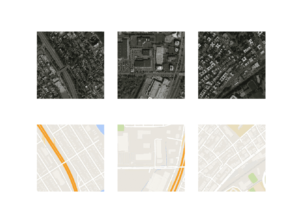
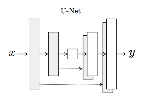
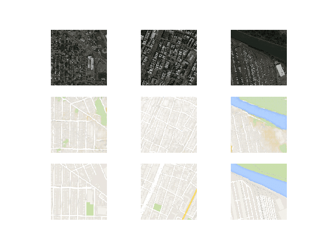
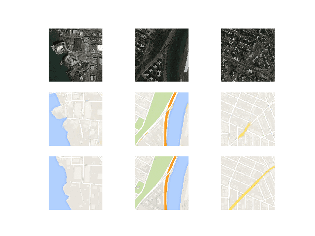
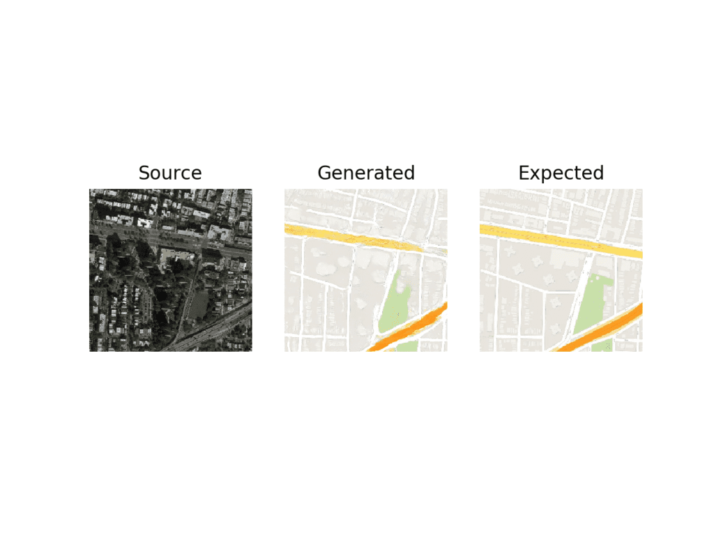
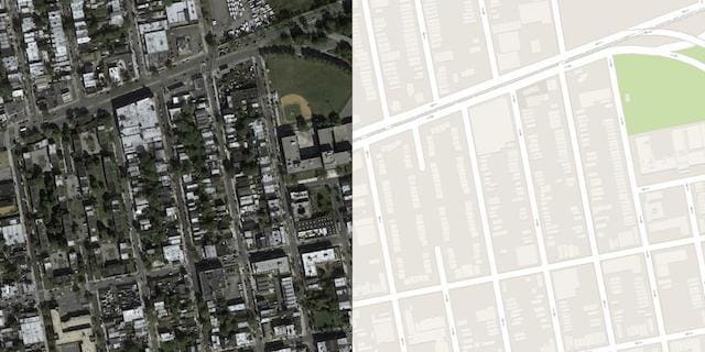
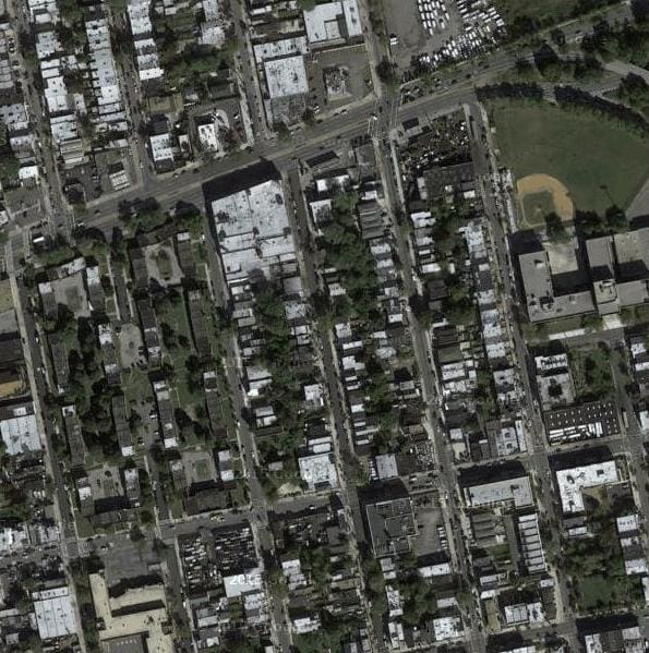
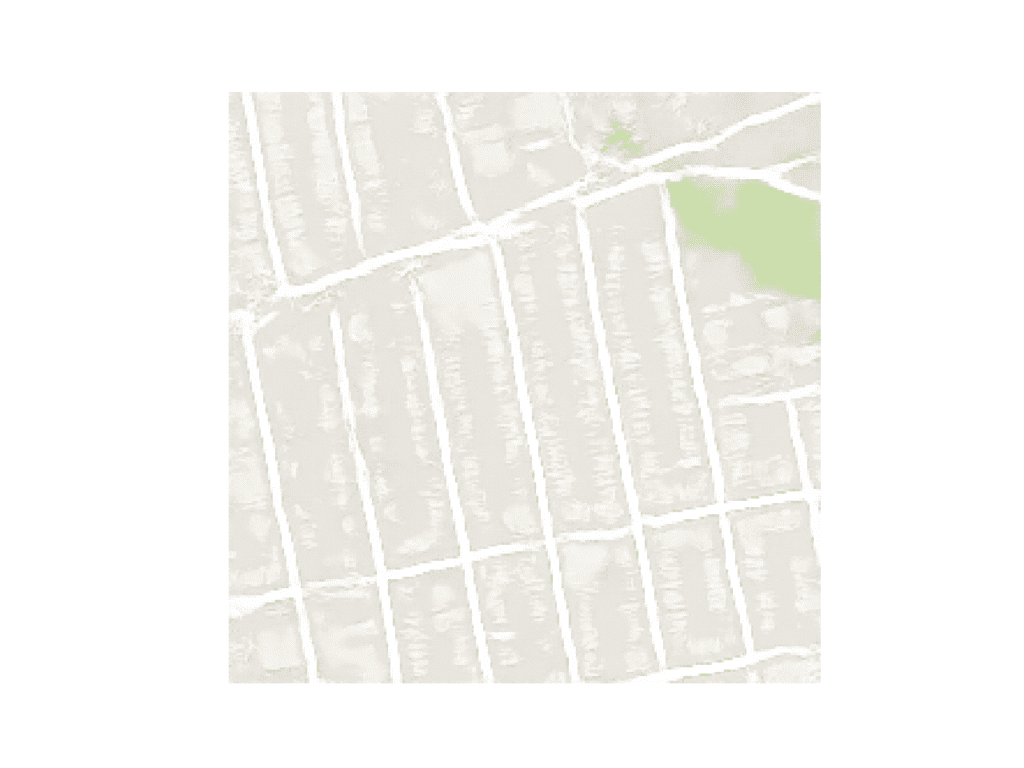
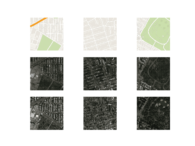
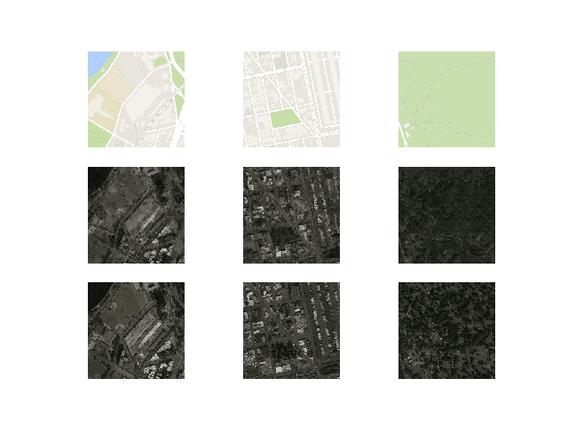

 From Scratch with Keras")


Amazing tutorial. Detailed and clear explanation of concepts as well as the codes.
Thanks & Regards
Thanks!
From a digital signal processing viewpoint a weighted sum is an adjustable filter.
Each layer in a conventional artificial neural network has n of those filters and the total compute is a brutal n squared fused multiply accumulates.
A fast Fourier transform is a fixed (nonadjustable) bank of filters, where each filter picks out frequency/phase.
There are other transforms that act as filter banks too, such as the fast Walsh Hadamard transform and these often require far less compute (eg. nlog(n)) than a filter bank of weighed sums.
The question then is why not use an efficient transform based filter bank and adjust the nonlinear functions in a neural network by individually parameterizing them?
Ie. change what you adjust:
https://github.com/S6Regen/Fixed-Filter-Bank-Neural-Networks
https://discourse.numenta.org/t/fixed-filter-bank-neural-networks/6392
https://discourse.numenta.org/t/distributed-representations-1984-by-hinton/6378/10
Perhaps test your alternate approach and compare the results Sean?
It seems to me that the discriminator is not a 70×70 PatchGAN, since the 4th layer should not be there. With that layer it seems like the discirminator is a 142×142 PatchGAN. Please correct me if I am mistaken.
I believe you are mistaken.
You can learn more about the 70×70 patch gan in greater detail in this post:
https://machinelearningmastery.com/how-to-implement-pix2pix-gan-models-from-scratch-with-keras/
That example has the same structure, 6 layers of Conv2D (including the last one). But when looking at the beginning of the post where You are calculating the receptive field with 5 layers of Conv layers. The calculation also states that there are only 3 layers of Conv2D with a stride of 2. I believe that the layer named C512 should be the second to last layer.
I believe the implementation matches the official implementation described here:
https://github.com/phillipi/pix2pix/blob/master/models.lua#L180
Hi Jason, thanks for the great tutorials. I agreed with Villem that the current discriminator model is a 142×142 PatchGAN. For a 70x70PatchGAN, I think it should be only 3 layers with 4×4 kernel and 2×2 stride (remove the C512).
If anyone else has the same confusion with me, please let me know. thanks:)
Thank you all for the feedback!
Sorry what’s the link?? This link is the same as the original one.
Thanks for the tutorial.
My question is in original paper they are giving the direction as configurable parameter.
But in your implementation I am unable to see that one.
How can do that for both direction.
Please explain
I show how to translate images in both directions in the above tutorial.
Many thanks for this amazing tutorial!
PS “There are 1,097 images”… and then there are saves every 10970 steps, and 109700 steps overall
Thanks.
Fixed.
Thanks for an amazing tutorial
How we use GAN for motion transfer or which type of GAN will best for Motion Transfer?
I don’t know off hand sorry, perhaps try a search on scholar.google.com
Hello, thanks for the great article.
I have one question, but why you scale the image to [-1, 1] instead of [0, 1]?
Does this make the model behave differently?
Because the generator generates pixels in that range, and the discriminator must “see” all images pixels in the same range.
The choice of -1,1 for pixels is a gan hack:
https://machinelearningmastery.com/how-to-code-generative-adversarial-network-hacks/
Hi sir, is it possible to train this model with inputs and output of different sizes?
For example, I have 3 image a,b,c with size 50x50x3. I want the model to generate c from a,b. First I append a and b to get d with size 50x100x3, then use d as input, c as output
Yes, you can use different sized input and output, although the u-net will require modification.
Could you give me some more details about how do I need to modify U-net in my case ? I’m not very familiar with this texture
Sorry, I don’t have the capacity to prepare custom code for you.
Perhaps experiment with adding/subtracting groups of layers to the decoder part of the model and see the effect on the image size?
I know you are very busy so I didn’t ask for custom code, I just need something to start with. Thank for the suggestion sir !
Perhaps start with just the function that defines the model and try playing around with it.
Did you find a solution for this? I am struggling with the same issue. Thanks
Hi Jason,
First of all, thank you very much for posting this tutorial, I learned a lot from it.
I have a question.
Do u think if I leave the picture resolution as it is rather than compressing them.
The performance is gonna be better? As my pictures between translation is very minor.
Thank you!
David
Thanks, I’m happy that it helped.
Interesting idea. You mean likely working with TIFF images or other loess-less formats?
Probably not, but perhaps test it to confirm.
Hello,
How can I increase speed of training? It uses very small portion of gpu memory.
Some ideas:
Use less data.
Use a smaller model.
Use a faster machine.
I am using a machine with 8 gpus (8 X p4000) 🙂
I mean, for example, while training on darknet, changing batch size directly affects gpu memory usage. But this codes use only 100 mb of each gpu. And batch size doesn’t affect it. So I need an adjustment just like on darknet so that I can use full capability of gpus.
Thanks
I see, I’m not sure I can help sorry.
Swapping out the training data for the SEN1-2 dataset had amazing results. I can now translate Sentinel 1 images to RGB Sentinel 2! Many thanks for such a thorough tutorial.
Well done!
I would love to see an example of a translated image.
Hi Jason,
Thank you so much for your great website, it is fantastic.
I was wondering what your opinion is about the future research direction for this area of research?
Thanks
Thanks.
Sorry, I don’t have thoughts on research directions – I try to stay focused on the industrial side these days.
Awesome tutorial on Pix2Pix. Your other GAN articles were great too and very helpful. After reading your tutorials, I was able to implement my own Pix2Pix project. All the code is on my GItHub. https://github.com/michaelnation26/pix2pix-edges-with-color
Thanks.
Well done, that is very impressive!
– python version: 3.6.7
– tensorflow-gpu version: 2.0.0
– keras version: 2.3.1
– cuDNN version:10.0
– CUDA version:10.0
mnist_mlp.py (https://github.com/keras-team/keras/blob/master/examples/mnist_mlp.py) works perfectly but code which is given below gives me this error:
tensorflow.python.framework.errors_impl.UnknownError: Failed to get convolution algorithm. This is probably because cuDNN failed to initialize, so try looking to see if a warning log message was printed above.
[[node conv2d_7/convolution (defined at C:\Users\ACSECKIN\Anaconda3\envs\tensorflow\lib\site-packages\tensorflow_core\python\framework\ops.py:1751) ]] [Op:__inference_keras_scratch_graph_4815]
Function call stack:
keras_scratch_graph
Perhaps try running on the CPU first to confirm your environment is working?
Code works with CPU. But I want to run in the GPU to complete in less time. CPU time is about 16 hours. I am open to any alternative to decrease the training time.
That is odd. I ran the examples on GPU without incident, specifically on EC2.
Perhaps try that?
Based on my experience, I receive this error message when my GPU does not have enough memory to handle the process. Maybe try reducing the computational workload by using a smaller image? If not, use CPU if you are fine with it.
Great suggestions!
Hi guys,
It takes 8 hours to train the model on GPU (Floydhub).
But several different models were saved in the process.
Can you explain why?
Perhaps try training on a large ec2 instance, it is much faster.
Models are saved periodically during training, we cannot know what a good model will be without using it to generate images.
Thanks for the tip!
Thought that more epochs give better results, since GAN`s cannot converge… so by theory no over fitting.. but I am new in the field, so I will look more into it 🙂
Not with GANs. Perhaps start here:
https://machinelearningmastery.com/start-here/#gans
Thank you for your awesome post, it is really detailed and helpful! I have a question about normalizing between [0, 255] to [-1, 1]. My images are single channel and the maximum and minimum pixel values vary for each image, from 0 to around 3-4 (depends on the image). How should I go about normalizing the images? Should I take the maximum of the whole batch of samples and normalize, or should I take the maximum for each sample and normalize each individually?
Also, when translating new images, what would be the values of image? Would it be between -1 to 1? If yes, how should I “denormalize” the values to the original? Thank you for your help!
Thanks.
I recommend selecting a min and max that you expect to see for all time and use that to scale the data. If not known or it cannot be known, use the limits of the domain (e.g. 0 and 255).
Thank you for your suggestions! How would you suggest I “de-normalize” the data during testing? Should I use the same range (I am taking the range from the training data) and reverse the process on the test data?
Yes.
Hi Jason,
Thank you very much for sharing such an in-depth analysis of Pix2Pix GAN. It is really helpful for early career researchers like me who don’t have a CS background. I thought of applying this fro solving and inverse problems in Digital Holographic Microscopy and I am now intrigued by the preliminary results I have got. As you know, the output of the model is a translated image, hence it is not possible to calculate the model accuracy. I am looking for an image quality metric such as SSIM. Do you have any suggestions?
Thank You,
PS: As this post helped me enormously, I would like to cite your works on GANs in the future.
You’re welcome.
That sounds very cool! Perhaps one of the metrics here would be helpful:
https://machinelearningmastery.com/how-to-evaluate-generative-adversarial-networks/
Hi! Currently implementing this with images with shape (256, 512, 3) and keep running to an error as follows:
“ValueError: A target array with shape (1, 16, 16, 1) was passed for an output of shape (None, 16, 32, 1) while using as loss
binary_crossentropy. This loss expects targets to have the same shape as the output.”I assume that this is due to the downsampling? Any help would be appreciated
Perhaps start with square images, get it working, then try changing to rectangular images?
Hmm, alright! Could you explain why you use target_size=(256, 512) instead of (256, 256)?
The images are 256×512 – as they contain the input and output images together.
We load them and split them into two separate square images 256×256 when working with the GAN.
The discriminator error seems to be going to zero pretty quick, any tips to avoid this?
Perhaps try running the example a few times and continue running – it may recover.
Thank you for this tutorial and simple code. I used it to perform image-to-image translation from Köppen–Geiger climate classification map ( https://en.wikipedia.org/wiki/K%C3%B6ppen_climate_classification ) to real satellite data, with truly amazing results, but I have a question.
In my strategy I create near one thousand pairs of 256×256 tiles from the Köppen–Geiger map (present in the Wikipedia article above), and a high-resolution satellite map of the Earth. In order to minimize deformation on tiles pairs near poles I use orthographic projection. This gives me nice pairs of image for GAN training (see https://photos.app.goo.gl/eGvpXghUtCB9kqkX6 ).
I trained the GAN until the end (n_epochs=100) with amazing results. Using training data give truly convincing satellite map validation (https://photos.app.goo.gl/a4EV6Gh15hAnYokm7). Even with hand-painted or with source image converted from a random image into Köppen–Geiger colormap, results are very nice (https://photos.app.goo.gl/eGbFmTH7YqYi4xfu5).
However I noticed that the result lacked of “relief” effect. Moreover, on large landmasses where the climate does not change but the topography noticeably affects the satellite view (e.g Tibetan Plateau or the Grand Canyon), the model results in “flat” satellite views.
As the climate map is composed of only 29 different indexed colors (plus the one I added for oceans), a simple label-to-image translation could be used, instead of using a full RGB climate image as input.
So my idea was to store a heightmap of the earth on the first channel of the input image, and the normalized indexed climate color on the second channel. The third channel is kept unused. It results in a Red-Green image where the Red channel is the heightmap and the Green channel is normalized climate index (see https://photos.app.goo.gl/cN1cmCNLSXwwqzNB9).
The problem is that training with this input images give bad results compared to my first try (only climate date). Results were already convincing after 30 epochs in my my first try, with smooth transition between climates, why here the boundaries are clearly visible in generated images (see https://photos.app.goo.gl/Q1vjjeY8ewWrCZYv5 ).
I tried to run the training several times to ensure that it was not purely bad luck, with the same result.
I don’t understand because climate index can clearly be stored on one channel without information loss, and heightmap provides additional data, so it should improve the results. Is it simply because it needs more epochs ?
Thank you in advance and sorry for the long post and for my english, it is not my native language.
Well done!
Very cool application.
Two thoughts off the cuff. One would be to make image synthesis conditional on two input images (source and the height map). A second would be to have 2 steps – one step to generate the initial translation and a second to improve the generated image with a height map.
I’m eager to hear how you go!
Thank you very much ! The aim is to develop a tool for worlbuidling and create realistic maps of imaginary planets (following Atrifexian’s tutorials https://www.youtube.com/watch?v=5lCbxMZJ4zA&t=1s ).
I used the idea of using R and G channels for heightmap and climate following this thread concerning the pytorch implementation : https://github.com/junyanz/pytorch-CycleGAN-and-pix2pix/issues/498. They recommend to concatenate the input images, but it seems that your code is limited to 3 channels and as I’m a complete beginner I still don’t know how to use more than one image as input.
However it seems indeed that training on more epochs actually gives good results with my method. Maybe 100 is not enough, so I restarted it with a limit of 1000 epochs. However I have to redo the first 100, an I run the code on Google Colab which seems to be very unstable (I only managed to reach 100 epochs twice).
Do you have a tutorial on how to make complete checkpoints in order to continue the training in case of crash ? If I understand well, your summarize_performance function only save the generator model, so we should have to save the whole gan_model and reload it for later training. Do you have documentation or examples concerning this ?
Thank you so much for your tutorial. I’ll keep you informed on later developments !
Yes, the above code already saves the model every n steps.
See the summarize_performance() function.
Should i approach this the same way if i have images containing white backgrounds? Similar to the edges2shoes dataset?
Perhaps test it with a prototype?
For some reason i end up only with blank white images…
Hello,
Thanks for the wonderful tutorial, Please how can I adapt the generator and the descriminator in order to make a transition from matrix (2,64) into matrix(2,64)
Sorry, I don’t follow.
Thanks Jason for great post!
I have tried this code, but images do not appear to be good enough, and discriminator loss becomes 0 after 10-15 epochs.
Perhaps try using a different final model or re-fit the model?
I want to continue training from the last checkpoint stored. Can you help me in resuming the training of a model from last checkpoint.
Yes, load the model as per normal and call the train() function.
I have a dataset consisting of 216 images. I trained for 100 epochs but unfortunately the results are not good. Can you help me how can I improve the results?
Yes, try some of these suggestions:
https://machinelearningmastery.com/how-to-code-generative-adversarial-network-hacks/
Thank you for this wonderful tutorial! It has been extremely helpful. I was wondering if you had considered data augmentation?
For GANs, not really, in general, yes:
https://machinelearningmastery.com/how-to-configure-image-data-augmentation-when-training-deep-learning-neural-networks/
Thanks!
This is probably a newbie question, but I am new to GANs. In my limited experience with deep CNNs, I used the validation data during the training process to sort of evaluate how well it was “learning”> I then had another dataset I called the “test” dataset that I used after the training process was complete. Here it seems like you don’t use any validation during the training process. And what you call validation is what I call the test dataset. Is that something unique to GANs or can validation be included in the training process?
No, I often use tests sets for validation to make tutorials simpler:
https://machinelearningmastery.com/faq/single-faq/why-do-you-use-the-test-dataset-as-the-validation-dataset
Hi! Im running this on Titan V and it seems to be running extremely slow. Any ideas as to why?
Training GANs is slow…
Perhaps check you have enough RAM and GPU RAM?
Perhaps compare results on an ec2 with a lot of RAM?
Perhaps adjust model config to use less RAM?
I suggest using google colab. You can use their GPUs for training. It’s much faster!
GPUs are practically a requirement when working with GANs.
sir can i know how you downloaded the images of satellite and maps can you please help me to download my own dataset for this project
See the section of the above tutorial “Satellite to Map Image Translation Dataset” on how to download the dataset.
Hi Jason,
From the theory, we understand that dicriminator learns the objective loss function.However referring to define_GAN(),line 56 in the code, I am not able to see the object loss learnt by discriminator getting passed to GAN model. I see that the model doesnot converge as expected
Thanks and Regards,
Vaibhav Kotwal
We create a composite model that combines G and D so that G is trained via inverse corrections to D.
Perhaps see this:
https://machinelearningmastery.com/how-to-code-the-generative-adversarial-network-training-algorithm-and-loss-functions/
Thanks for the great tutorial. I need help with something. I want to see accuracy metrics for both train dataset and test dataset throughout the training process. And I want to see this for each epoch, not for each steps. Like a standart CNN model training procedure. How can add this things to code ? I couldn’t apply it because it is different than standard CNN codes. I would really appreciate it if you answer. Thank you.
Accuracy is a bad metric for GANs.
See this:
https://machinelearningmastery.com/how-to-evaluate-generative-adversarial-networks/
Can pix2pix Gan save and load againt without training again
Yes, see this tutorial for an example:
https://machinelearningmastery.com/how-to-develop-a-pix2pix-gan-for-image-to-image-translation/
Yes,thank for your reply!!And I want to ask another questions!!Can the other kind of GAN versions save and load?
Yes, they are all Keras models that can be saved and loaded.
Hi Jason,
Thanks for the great tutorial. I have a problem with image scales. In first step, after splitting the input images, I check the image size, instead of of 256*256 pixel they are 134*139 with background. Also, at translation a given standalone image using by model step, the output should be 256*256 same as input, but I get 252*262 output again with background.
I was wondering if you would mind letting me know where is the problem?
Thanks in advance
Ehsan
I don’t know the cause of your fault. Sorry.
Great work Jason. Just one question: do you believe that this approach could work using a RGB satellite image against its mask image, to make some kind of image segmentation ?
Thanks in advance
Perhaps try it. Prototypes are a fast way to get answers.
I mean, the mask image would have just 2 colors (yes/not) … this was my concern. Thanks
You can add two ‘dummy’ layers to the mask image, so that it is compatible as a target image to the RGB source image. Your RGB image as numpy array will be in the shape of (nr images, width, height, nr bands) where nr bands is three. Your mask image will be in shape (nr images, width, height, nr bands) where nr bands is one. So if you add two bands to the mask image, with e.g. only -1 values, then they are compatible.
It is an interesting article publish here. I am new using this, i want some question for the first script for clear explanation :
1. I saw the loaded data is maps in train and test folder. I want to know which 3 sample was loaded from the folder train? because the results was : (1096, 256, 256, 3) (1096, 256, 256, 3). I understand 1096 is the certain amount of image in that folder. and 256 I still dont understand because when I open picture 256 is not the same as the it was loaded.
2. I saw the folder contain image in train and test. I want to ask the train, example 1.jpg it contains two image from satellite. May I know how to develop the left picture and the right picture or it develop itself? Also in test does it develop itself or have to save it first?
Need some explanation for preparing using it in the future. Thank you
The images are 256×256 squares with 3 color channels. You can learn more about loading images here:
https://machinelearningmastery.com/how-to-load-and-manipulate-images-for-deep-learning-in-python-with-pil-pillow/
Sorry, I don’t follow your second question, perhaps you can elaborate?
thank you for replying. For my second question I saw the folder train and test contains an image. So the question come up :
1.Does the image build itself?
2. If No, how do you make the images side by side that contains two image in one image.
Thank you very much.
The tutorial shows how to load the images and prepare them for modeling.
hi thank you for your work !
I need your help,I need the same model but the input of the generator is one channel and not three .
I have tried to change it but it does’nt work .thank you
Sorry to hear that.
Perhaps confirm that your images are grayscale (1 channel), then change the model to expect 1 channel via the input shape.
Hi! I wanted to train myself. I prepared them just like in this tutorial. Size X1 and X2 are the same. Data display works. But I get this error:
‘Got inputs shapes: %s’ % (input_shape))
ValueError: A
Concatenatelayer requires inputs with matching shapes except for the concat axis. Got inputs shapes: [(None, 2, 2, 512), (None, 1, 1, 512)]What have I done wrong?
I don’t know sorry.
Have you been able to solve this problem. I get the same issue.
This is probably because your input size is not divisible by 256.
hello I have this problem I dont know why :
ValueError: Graph disconnected: cannot obtain value for tensor Tensor(“input_14:0”, shape=(?, 256, 256, 3), dtype=float32) at layer “input_14”. The following previous layers were accessed without issue: [‘input_15’]
Perhaps confirm that your keras and tensorflow versions are updated?
Hi. I tried to use a different dataset using this code. Specifically the edges2shoes dataset but i was not able to convert it into npz file. Everytime i ran into memory error. My ram is 16GB still that was not enough. I managed to create multiple npz files though. How should i proceed?
Also could you be kind enough to make tutorial of Tensorflow/Keras of pix2pixHD since it is much more accurate and better in side by side tests compared to normal pix2pix.
Perhaps use a sample of the data?
Perhaps use progressive loading?
Perhaps use an ec2 instance wth more ram?
Thanks for the suggestion.
Thanks I think your tutorial here https://machinelearningmastery.com/how-to-load-large-datasets-from-directories-for-deep-learning-with-keras/ will be helpful in my case.
I am using my own machine not AWS instance.
Great!
Hi Jason. Great Article. Good explanation. Your articles gave me a good overview and starting point when I started developing my own networks. But I have two questions:
1:) From what I can see the original code on Github seems to be slightly different to your code in this article when it comes to how you connect an encoder and a decoder layer. On Github data from an encoder layer passed to a decoder layer (via skip-connection) is unactivated, meaning that the data is passed directly after the convolution(or batch norm/dropout), in contrary to the solution here. Is this a mistake or variation ?
2.) What does the flag ‘training=True’ do when calling batch normalization layer or dropout layer ?
Thanks in advance.
Perhaps. I thought I had the architecture spot on based on the paper and the released code.
Training=True causes the layer to think it is always in training model. E.g. normally batchnorm and dropout operate differently in training vs inference. More here:
https://machinelearningmastery.com/how-to-implement-pix2pix-gan-models-from-scratch-with-keras/
Hi Jason,
thank you very much for this tutorial, it’s awesome!
I have the problem that you mentioned at the end of the article. D1 loss goes to zero after 80-90 steps. Could you explain me why this happens and how can I solve it?
In addition to this, I can see that only one image is used in every iteration (one real,one fake) where n_batch = 1. Shouln’t we use more than one pair of images to train in each step?
# select a batch of real samples
[X_realA, X_realB], y_real = generate_real_samples(dataset, n_batch, n_patch)
Thank you very much!
Yes, this is probably a failure mode:
https://machinelearningmastery.com/practical-guide-to-gan-failure-modes/
You can try fitting the same model again, save models to file along the way.
You can try tuning the model architecture or training algorithm:
https://machinelearningmastery.com/how-to-code-generative-adversarial-network-hacks/
So, the model as it is in this example is not going to work properly? This link is not a pixtopix architecture. I tried also the example and work perfectly for cGAN and GAN with fminst, but the problem is this Pixtopix architecture.
The example does work correctly, but you may need to train it a few times.
GANs are unstable by definition.
I’ve seen that there are specific codes in your book about this. Is a more complete example for pixtopix? Or is it the same?
The examples of pix2pix in the book are based on this example.
long live 100 years …. superb tutorial with clear explanation
Thanks!
anyway to use a keras data loader/generator for on the fly image loading dsirng training? say for example your training size is really large and loading all at once would result in out of memory errors? thanks so much for all your tutorials, they are incredbile!
Yes, see this:
https://machinelearningmastery.com/how-to-load-large-datasets-from-directories-for-deep-learning-with-keras/
Hi Sir,
First of all i read your all tutorials. You are helping me more than my consultant. Thank you so much.
I am new at Gans. Sorry for my quesitons. But i cant understand how i test this model?
I will use validation set okey.
After training model i wont give target, just give source image?I cant get it.
Or only ı load model and train with validity set?
Omg i cant explain myself. I hope u are understand me.
You’re welcome!
Evaluating GANs is challenging. We do not use a validation set. Instead we generate images and look at them and see if they are good enough.
thank you for your answer Sir,
i wanna try pix2pix gans for image enhancement.
I’l use source images are low contrast, targets are high contrast ,what do you think? i’m trying to improve thermal image.
I hope this system will work.
Sounds great!
Here in Discriminator what is the need for Concatenating Source and Target images ? What effect would it have ?
Sorry, which section are you referring to? Where (which section/line?) do we concatenate images?
In discriminator. where we are concatenating Source Image and target Image.
Actually I’m building a GAN model color transformation from Gray to RGB.
My discriminator and Generator model’s loss falls to zero. So wanted to know that what particular effect does the Concatenation have for discriminator. And if you have any advice for my model than tell it too.
THANKS in advance…
Here we are training a conditional model, e.g. generate a target image conditional on the source image.
E.g. it is the purpose of the model.
Hello. I compared the images from the summarize_performance() to predictions on unseen ones, which turned out to be quite horrible. Can you suggest some ways to tackle this problem ?
Try training the model a few times, save many times during each run, choose a model that generates good images.
Hi,
How can I use the generator model to predict any size of images? I mean not just squres sizes. Is there any way at all?
You will have to change the generator/discriminator and also the training dataset to the desired size.
Thank you for the awesome post. I have 2 questions if you can answer please.
First question, you have mentioned:
“In this case, we will use the model saved at the end of the run, e.g. after 10 epochs or 109,600 training iterations.”
Shouldn’t the training iterations be 10,960 after 10 epochs.
Second question, what is the rationale behind using random index to generate real and fake samples? Why can’t we simply iterate over all the samples one by one to make sure no image is missed or used more than once in 1 training step?
Images are generated after every 10 epochs, it runs for 100 epochs, meaning we save 10 models along the way. Yes, that is a typo, we used the model after 100 epochs. Fixed.
We can do it for all image, I wanted to work with one image, to show we can use the model ad hoc. Readers often find that step confusing so I must demonstrate it.
Hi!
thank you for the great tutorial, you helped me a lot!
i have just a question: am i doing something wrong or is it normal that for a X input i do not have a unique Y output.
Let me explain better: if i repeat n times the prediction i get n different Y images (i’m checking pixels differences).
I’m translating this this example to another application and having the exact same output everytime will make it works.
I tried to look for a random noise vector or something like that but it seems that this is not the case.
Recall we are using a GAN, so we have two models, the first predicts whether input images are real/fake and the second generates images conditional on another image.
If you are new to GANs perhaps start here:
https://machinelearningmastery.com/what-are-generative-adversarial-networks-gans/
EDIT:
” I’m translating this this example to another application and having the exact same output will make it works” *
Hi!
this tutorial helped me a lot!
i have just a question: is it normal that if i repeat n times the prediction, with the same input, i have n different outpus?
I’m checking directly changes in pixel values in Y outputs.
Yes, this is expected given the stochastic nature of some of the layers.
thank you for the reply!
I’m guessing that dropouts are introducing randomization, i’ll try without that.
Yes, also there are layers that inject noise directly.
i’m sorry if i seem annoying but i do not see layers that can introduce directly noise in the code you provided.
I see convs, batchnorms and concatenates.
Can you please tell me which layer is introducing noise directly?
i think that i have missed something about these layers but reading through the documentation it seems like i know them pretty good.
I really need to understand the position of these noise generator and remove them in order to use a GAN for my application (maybe it could be impossible but i wish to try =) )
Sorry, my mistake, I was thinking of a different GAN.
Thanks for the great tutorial.
I have one small doubt:
Do we traverse over the complete dataset?
We passed our entire dataset to the generate_real_samples function and everytime it chooses a random number, which could be same, if we traverse again and again.
So, we might not be traversing over the complete dataset in single epoch?
Please let me know your thoughts.
Thanks.
You’re welcome.
Correct. On average we cover the whole dataset many times.
So, there is a possibility of missing certain datapoints. This can become a problem if you have very less data points to work with.
So should I change the code to make sure, it traverse over entire data, or is it still ok, if we don’t do that ?
If you prefer. I’m not convinced it makes a difference, but could be a fun experiment.
oh, ok no problem!
i think that i will investigate stochasticity trought the different convs and batch norm in order to make the net able to predict the same Y from an X input.
best regards
Thank you so much for this super clear explanation and code.
You’re welcome!
If I wanted to use an input with three colour channels and a target of four colour channels, can this be configured or is it best to just create an additional black 4th channel on the input?
I noticed some greyscale-to-colour models just use the same data in each channel to represent grey images so presumed it mush be easier to do this than make the model work with differing numbers of channels.
Also, thanks for the excellent resource!
Off the cuff I recall the images have to have the same number of channels. Perhaps experiment/research and see if you can deviate from this norm.
Thanks for this great post!
For your generator’s loss, how can I know if are you minimizing 1: log(1 – D(G(x))) or maximizing 2: log D(G(x))?
How can one change the loss function, any reading suggestions?
Some people say the choice of generator’s loss can help the model to not get stuck in early stages of training.
Good question, this may help you understand the loss function for GANs:
https://machinelearningmastery.com/how-to-code-the-generative-adversarial-network-training-algorithm-and-loss-functions/
You can see examples of alternate loss functions in tutorials here:
https://machinelearningmastery.com/start-here/#gans
Hello Jason,
What would be the optimal loss values (Generator and Discriminator loss) of a successful conditional GAN model? Are the values same as an unconditional GAN ? (i.e around 0.7 or 0.6, as mentioned in your unconditional GAN article)
Secondly, I have done the training of pix2pix for a certain image to image translation task in two different ways.
1st method: Trained the discriminator patch outcome against a matrix of real or fake labels (as mentioned in this article)
2nd method: The discriminator still gives a patch, but this time, the patch average was taken and was trained against a single value ( i.e avg value of the patch against a real or fake label).
During the training ( towards the saving of a good model), the first method, yields a patch avg value of about 0.4 for a real image pair and about 0.3 for a fake image pair.
But the second model, yields a patch avg value of about 0.0004 for both real and fake image pairs.
Both these models yielded a good quality image with its Generator and the Discriminator loss standing around 0.7 and 0.6 respectively. My doubt is why such discrepancy with the avg patch values even though both the models yields a good quality image? Secondly, an avg patch value of 0.0004 doesn’t make sense even though this model yielded a good translated image.(Because as far as my understanding, each pixel values in the patch for a real pair should be close to 1 for a real pair and 0 for a fake image pair. This would mean that the avg of the patches should also be close to 1 for a real pair and 0 for a fake image pair).
What should be the avg patch values for a good model? Any amount of insights into this would be greatly helpful. Hope I made sense.
Thanks!
GANs don’t coverage, so there is no optimal loss values, you can learn more here:
https://machinelearningmastery.com/faq/single-faq/why-is-my-gan-not-converging
Comparing loss between models/runs is not valid.
GANs are hard to evaluate, subjective image quality is about the best we can do, although there are some metrics described here that might help:
https://machinelearningmastery.com/how-to-evaluate-generative-adversarial-networks/
Sir, Why exactly are we merging two images in discriminator ?? What effect does it have ?? And why are we not keeping just the colored image in Discriminator ??
The discriminator is given the input image and a target image and comments on whether the target is a real translation or a generated translation.
Can PIX 2 PIX GAN works for gray-scale images??
what if if we use the above same architecture for gray-scale source and target images.
Modification of the model architecture is required.
I used different data of source and target image. My source and target images are gray scale.
But when i run the code , the discriminator loss is going to zero with very few iterations but generator loss is very high that is ,,9782.150 up to so on.
It cannot be decreasing ….What can i do ??
GAN loss does not converge, you can learn more here:
https://machinelearningmastery.com/faq/single-faq/why-is-my-gan-not-converging
I have different source and Target images. And My source and target images are in gray scale but my discriminator loss is going to very low reaches to zero but generator loss is very high.
what can I do now ?? Can Pix to Pix GAN work for gray scale images.
You may need to tune the model – explore – in order to discover how to best modify the model architecture to support grayscale images.
What sort of modification you think are required ?? Like the architecture won’t be U-shaped ?? Or is the loss that needs to be changed ??
It is hard to know – experimentation is required, perhaps start with tuning the learning rate with a similar network structure adjusted for the changed number of channels.
Hi!
Thanks for your great work!
I found your model above and tried with the cityscapes images. I trained ~3000 image pairs from segmentation to photographic pictures. First I convert the images to 256×256 and kept the 100 epochs, then trained with 250 epochs. The results were good, but blurry, so I converted the original 1024×2048 resolution images to 512*512 and trained them till 250 epochs.
The results didn’t really improve, but somehow I’d like to get less blurry pictures. I think increasing the number of epochs or the image resolution didn’t change a lot, so my question would be: Do I need to change on the architecture of the models? If yes, can you give me a hint what further layers should I use?
Thank you very much and keep up the good work!
You may need to experiment with the model architecture and learning hyperparameters in order to discover what works best for your specific dataset.
Thanks for your reply, Jason.
Can you give me a hint, what architectural changes I should start with if I want to train with 512×512 resolution images or even bigger instead of 256×256? More conv2d layers, dropout layers or multiple discriminators/generators as in pix2pixhd?
Thank you.
A good approach is to scale the number of blocks up or down from the current to meet the desired image dimensions.
I would encourage you to experiment and observe the effects on input/output shapes to get a feeling for it.
dataset = LoadRealData (‘C:/Users/Eeshwar/Desktop/deep learning/maps11.npz’)
print(‘Loaded’,dataset[0].shape, dataset[1].shape)
Imgshape = dataset[0].shape[1:]
dmodel = DiscriminatorModel(Imgshape)
gmodel = GeneratorModel(Imgshape)
ganmodel = GANModel(dmodel,gmodel,Imgshape)
TrainModel(dmodel,gmodel,ganmodel,dataset)
Loaded (1096, 256, 256, 3) (1096, 256, 256, 3)
WARNING:tensorflow:Discrepancy between trainable weights and collected trainable weights, did you set
model.trainablewithout callingmodel.compileafter ?InvalidArgumentError: data[0].shape = [4] does not start with indices[0].shape = [2]
[[{{node training/Adam/gradients/gradients/loss_3/dense_2_loss/Mean_grad/DynamicStitch}}]]
Sir could you please help me to resolve this issue. I Thank You in advance
Sorry to hear that, this will help:
https://machinelearningmastery.com/faq/single-faq/why-does-the-code-in-the-tutorial-not-work-for-me
Hello sir, the tutorial was great, but i have 2 questions.
1) In the define_discriminator() function, you have set the loss_weights parameter to 0.5, to slow down the training of discriminator. Can’t we reduce the learning rate of the discriminator model to slow the training, instead of specifying the loss_weights parameter?
2) In the define_gan() function, why was there even a need to specify loss_weights parameter over there?
Thanks.
Perhaps try it an see.
We do se a loss_weights for the gan.
Ok , i will try reducing the learning rate instead of specifiying the loss_weights parameter in the define_discriminator(). But i am sorry, but i still do not get the answer of the second question, i.e, why do we need to specify loss_weights parameter in the define_gan() function.
To match the implementation described in the paper.
It has the effect of giving most attention to L1 and a tiny bit of attention to cross entropy.
This is explained in that section of the tutorial, perhaps re-read?
Hello sir, thank you for the great tutorial !
I am new to Machine Learning,
I want to change the clothings of people in images or videos. So i should train pix2pix on a clothes dataset ?
The second question is that i dont want to change anything else in the image except the clothes, so if i apply pix2pix on the image it will change everything, how can i target only clothing in a image ?
Thank’s again for your great work !
Perhaps try it and see how well it can do.
Hi,
I have trained the exact model outlined in the tutorial with the same data-set quite a few times and the losses of the discriminator are always consistently 0.000 after around 5000 steps. Looking at the loss to more significant figures, shows that the loss is greater than zero, hence, when you state that, if the discriminator loss stays at zero for a long time then there is training failure, do you mean zero to 3 decimal places (0.000)?
The generator still improves after the discriminator loss states 0.000, however I presume that the discriminator is no longer having a significant impact on the training of the generator.
Thank you for the great tutorial, it helped a lot!
Zero loss indicates a failure mode:
https://machinelearningmastery.com/practical-guide-to-gan-failure-modes/
Recall that GANs do not converge:
https://machinelearningmastery.com/faq/single-faq/why-is-my-gan-not-converging
Are you saving models along the way during training?
Are you able to inspect the progress of training, does it get good then go bad or is it bad the entire time?
I am saving the model every 5 epochs, and the predicted images do improve slightly during training, and by the end look reasonably good, (I presume that the discriminator hasn’t had an impact on the quality and it is just the generator improving by itself).The losses of both the discriminator and generator decrease to start with, but the discriminator slowly decreases to 0 and the generator stays pretty low (between 1 and 5).
I have assumed that the discriminator is too good at determining the real and fake images, as I have removed a few layers from it and it’s loss doesn’t decay to 0 during training.
Interesting. Thanks for sharing Alex.
I have around 3700 images to train on.
Can you roughly guide for the hyperparameters(like n_epochs,n_batch to be set as I’m encountering the following issue?
Please help in resolving it.
/home/reshmajindal/.local/lib/python3.6/site-packages/keras/engine/training.py:490: UserWarning: Discrepancy between trainable weights and collected trainable weights, did you set
model.trainablewithout callingmodel.compileafter ?‘Discrepancy between trainable weights and collected trainable’
Killed
https://machinelearningmastery.com/faq/single-faq/why-does-the-code-in-the-tutorial-not-work-for-me/
I even tried all of this, but didn’t work.
We cannot know the best way to configure the model, instead we must use experiments to tune and discover what configuration works best for a given dataset.
These tutorials will teach you:
https://machinelearningmastery.com/start-here/#gans
Thanks for this GREAT detailed tutorial. One question I have in mind is how to adapt the model to input different sizes of images? i.e. if the training/validation images have different height and width values?
You’re welcome.
Typically images are all resized to the same width and height expected by the model.
resizing is a bit flexible term 🙂
cropping big images leads to loosing some information. enlarging small images might lead to blurry images. Super-resolution is computationally expensive and needs auxiliary models. What do you think the good way to “resize” images to work properly with this model ?
I recommend exploring many diffrent approaches and discover what works best for your specific project.
YES!! the best way to find out is by doing it! this why I feel addicted to this machinelearningmastery :p
Thanks!
Is there a way to input your own image? I haven’t seen any demonstrations that are able to input your own image and I have tried doing it myself but to no avail.
Yes, the last part of the tutorial shows this.
Hi everyone. Thank you for super guideline for implementation. I have one question. Can i generate 1024×1024 px image by using pix2pix-GAN?
Perhaps try scaling up the model for large images and see what kind of results you get.
I would expect quality to fall off. It might be easier with a model based on the progressive-growing architecture.
By the way, my dataset image size is smaller than 1024px
Hi!
It is a really good tutorial. I wish to apply this concept to my work. But I want to give some numerical parameters (say P1, P2, P3…) along with image as input and wish to get the image as output.
Can you guide me on how to change the code to implement this? Is it at all possible?
Thanks.
Perhaps take a look at some alternate GANs like conditional GAN or InfoGan:
https://machinelearningmastery.com/how-to-develop-an-information-maximizing-generative-adversarial-network-infogan-in-keras/
Thanks for this great tutorial.
Both losses for the discriminator has gone to zero in the first 100 epochs.
Can you help me?
Perhaps restart training and stop once the generated images are good enough.
Great tutorial sir.
I have my both discriminator loss heading to zero, in the first 200 steps. I cannot solve my issue and had run many times. Can this be a problem with the version?
Perhaps try changing/tuning the learning hyperparameters of the model.
Perhaps try some of the suggestions here:
https://machinelearningmastery.com/how-to-code-generative-adversarial-network-hacks/
Thanks for the reply sir. I will try that.
But why shouldn’t it work if the code is same as above?
The model uses a stochastic learning algorithm, you may need to run the example a few times to get a good result.
you can learn more about this here:
https://machinelearningmastery.com/faq/single-faq/why-do-i-get-different-results-each-time-i-run-the-code
Great tutorial!
I am trying to apply this architecture to a MRI image-to-image translation task. I have two questions regarding the architecture for this purpose:
1) After slicing the MRI data to 2D slices. Do I need to convert the NIFTI-files to JPEG or can I directly save them as npz (compressed numpy array)?
2) MRI images are grayscale whereas the example code in this tutorial uses RGB images. What would change in the architecture of the tutorial to deal with grayscale images?
Thanks Jason.
The model takes image data as numpy arrays. I don’t know if converting data to jpeg first is required for your data.
Yes, you can adapt the model for grayscale images, e.g. change the number of channels for input images to D() and output from G().
Jason,
What an incredible article. I reproduced your methodology on a research project on mechanical networks, where the model learns to draw mechanical linkages between parts of the system. It works perfectly, despite a small sample of training images.
I re-used one of your images (the Unet architecture of the Generator) on a blog post I made on Medium, carefully citing your article as source and your work as reference. You can check it out here:
https://adriensaremi.medium.com/develop-a-image-to-image-translation-model-to-capture-local-interactions-in-mechanical-networks-9c2f45230849
I wanted to make sure you approved the re-use of the image in question. Thanks again for you work here and more broadly on Machine Learning Mastery.
Thanks.
That’s fine, well done on your post!
Thank you for your great tutorial
I read a few posts about GANs and i realized GANs applyed in square images. is it right? can i use it for non-square images?
Yes, they can, bit square is much simpler.
Thank you for your great tutorial.
please how can I use GAN for deformable image registration?
Thanks Jason.
You’re welcome.
Perhaps start by checking the literature for existing approaches and try them first.
hi, Rekka, do you find any method to do with the deformable images? thanks
Hi,
Hope you are doing good.
I have tried your code and it works perfectly well.
I need to know, how about testing this module on a separate dataset,because i have found out that most of segmentation algorithms using gans include testing dataset also.
If i use a part of validation dataset ( and call it my test dataset) on saved model (e..g model_109600.h5) the results are fine. But if i use a different test dataset, the segmentation results are not desirable.
I would be glad if you can shed some light on this. Also please tell me, is there any way that this algorithm can be tested on a test dataset? If not, is there any reference that signifies that testing pix2pix for image to image translation is not a good choice?
Thanks
Thanks.
Sorry, I don’t have an example of combining GAN output with a predictive model – I don’t think I can give you good off the cuff advice on the topic. Perhaps check the literature.
Hey, really well explained, good job!
I have implemented similar cGAN for b&w image colorization. It is very hard to train, and somehow after many, many epochs on big datasets I got some ‘good enough’ results, but I wonder how can I measure accuracy for translated images?
Also during training and after finishing it my cGAN is resulting in very big Losses of gen like 10.0 and 2.0 at the end of training. Disctiminator’s loss is near 0 and peaking sometimes to even 3 or 5. How can I measure accuracy of trained model or during training?
Thanks
Thanks.
Good question, this may give you some ideas of how to evaluate a GAN model:
https://machinelearningmastery.com/how-to-evaluate-generative-adversarial-networks/
Hi Jason,
Thank you very much for detailed explanation with examples. It is very helpful.
I am trying to edit the code through notepad++ but it is giving me indentation error. Seems like there are a mix of spaces and tabs.
Can you please tell me what IDE or editor you used?
Apologies for a silly question.
You’re welcome.
This will help you copy the code correctly:
https://machinelearningmastery.com/faq/single-faq/how-do-i-copy-code-from-a-tutorial
Amazing tutorial, even more impressive that you’ve responded to every comment over year later! Quick question: you said that if either discriminant loss plateaus at 0 for an extended period of time that it has most likely failed and should be restarted. I am running it for the third time and both have landed on zero again, am I doing something wrong? Anything I can do to improve chances of it succeeding or just keep trying? (P.S. I am using different images and am using 2000 images as opposed to your ~1100 (still 100 epochs) but I assume that this does not affect the base of the model). Thanks in advance.
Thanks!
Sorry to hear that.
Perhaps try fewer epochs?
Perhaps try changing other learning hyperparameters?
Perhaps try adjusting the architecture?
Perhaps try some of the ideas here:
https://machinelearningmastery.com/how-to-code-generative-adversarial-network-hacks/
Just an update, tried some things you suggested, in the article as well as in the well appreciated comment, not much changed. Let it run just to see what would happen and even though the model read 0 for both discriminators for more than 6 epochs, it still gave me decent results, so I’m happy. Thanks for the amazing article and the helpful advice, will definitely be reading up on some of your other articles.
Thanks for the update and well done!
Hi, I love your whole blog and tutorials!
Just a question, Is it possible to train a model that uses 2 source images for one target?
For example from a traditional satellite image + an Infra Red (IR) image recreate the corresponding map?
Thanks a lot
Thanks!
I don’t see why not. I expect there are papers on exactly this – I recommend seeking them out to get ideas.
Thank you very much for the amazing tutorial!
My question is if it is possible to continue training from a saved model ? what would be the inputs of train function ? Thanks again
You’re welcome.
Yes, you can load the saved model and continue training. You can use the same code as the first round of training as a starting point.
Is this model applicable to generate super resolution data?
No, I believe there are more specialized models for that problem described in the literature.
Can you please share the link of some articles for those specialized models? for generating super resolution data.
You can search for papers on the topic here:
https://scholar.google.com/
What is the significance of converting the pixel values from [0, 255] to [-1, 1]?
Is it because of the tanh activation function being used in the generator model for the last layer?
This architecture can be used to matrix to matrix mapping as well. but a matrix might have pixel (arr[row, col]) values as real values (from [0, inf] instead if [0, 255]). In that case, what would you suggest for transformation (to [-1, 1])? Should that still be done?
Thanks,
Apologies for multiple questions.
Yes, exactly.
Yes, it is standard practice to use tanh for the output layer of gan generator models and to scale data to match the distribution of the activation function.
Thank you very much. I appreciate the responses.
You’re welcome.
I have noticed that in the code that the discriminator model is being compiled and the gan model is also being compiled but the generator model is not being compiled. generator is being saved. Whenever I load the generator model for prediction, it generate a warning saying
“No training configuration found in save file: the model was *not* compiled. Compile it manually”
Can you please guide me if it can affect model’s performance? seems like my models are not working.
After googling it I got a perception that it is just a warning but still wanted to check with you.
Thanks
No need as we are not training it directly. You can ignore the warning.
Thank you for the response.
I am fan of your site. Always thanks for your great article.
I would like to ask loss function that you utilize in the logical gan model. In your code block, 2 loss function was used in define_gan function.
model.compile(loss=[‘binary_crossentropy’, ‘mae’], optimizer=opt, loss_weights=[1,100])
If I understand correctly, ‘mae’ takes labels (true and predicted labels) instead of images. But in the pix2pix paper, l1 loss was defined as follows:
L1(G) =Ex,y,z[‖y−G(x,z)‖]
The output of G model is image and their loss function is defined based on differences between true images and generated images instead of labels.
Is it the same effect with labels instead of using images?
Yes, MAE is the L1 norm between image pixels.
Thank you for your answer.
Hi Dr. Brownlee,
In your last version there was a line in the define_gan method:
# make weights in the discriminator not trainable
d_model.trainable = False
my question is that it the discriminator is not trainable then how will it improve?
In current version of your code you have replaced it by following lines:
# make weights in the discriminator not trainable
for layer in d_model.layers:
if not isinstance(layer, BatchNormalization):
layer.trainable = False
if the weights are not trainable then how will discriminator learn and get better, and contribute to make the generator better?
my understanding was that weights are the ones that are supposed to be trained in the training process. Please correct me if I am wrong. Apologies as I am not an expert. I am learning through your articles and other stuff.
Thanks in advance.
The D is only not trainable when part of the composite model. This is called layer/model freezing. It is still trainable as as a standalone model.
Thank you so much Dr. Brownlee.
Hi Dr. Brownlee, if I want to have a higher learning rate for the discriminator and a lower one for the generator, say 2e^-4 for discriminator and 1e^-4 for the generator, should I just change the learning rate setting of the composite model?
Yes, the composite model is used to update the generator.
Let me know how you go with your approach.
Hi Jason,
Thank you for your great tutorial.
I just want to ask you one question: why during the inference we have to keep the batch norm and dropout in the training mode?
I understand that the dropout is performed to add some noise, but I thought it was necessary only for the training part.
Moreover, I have performed the training with a batch size = 1 and in the prediction phase I had applyied the generator to a volume of stacked images of dimension [N, 256, 256, 3] and the results were very different. Using a batch size = 1 in the prediction phase gave me better results. I think that this is correlated to the adoption of BN in training modality.
Thank you for your time
No. Batchnorm and dropout can are flipped to inference mode. Batchnorm will use learned mu and sigma and dropout will stop dropping out.
but the flag training is set to True for both BN and dropout, I think that this flag makes them work as during the training phase
Hi,
Is it possible to plot losses in realtime? I couldn’t manage to do it. Could you please help me?
Perhaps via tensorboard?
Hello, thank you for the sharing.
I’d like to know what is d1[0.362] d2[0.405] g[78.143] each loss value’s meaning?
Does it mean that is fake when discriminator’s loss value close to zero?
And what is the composite’s loss calue mean?
The values are hard to interpet.
Nevertheless d1 and d2 are the discriminators loss on real samples and fake samples (of “B”) respectively, and g is loss of the composite model on real samples.
This may help you interpret cross entropy more generally:
https://machinelearningmastery.com/cross-entropy-for-machine-learning/
Hi Jason,
Thank you very much for this informative article.
I have a question about a good GAN model to create more synthesis images from a small set of medical images? Is styleGaN good for this problem?
Perhaps trial a few methods and discover what works well or best for your dataset.
Hey,
If possible , can you please share the .h5 model after complete training. As I am trying but not able to train my model fully due to low computation power.
I have tried on colab too, but gets stopped after some time.
Sorry, I cannot share saved models.
Hey Jason,
This was an awesome tutorial.
I wanted to try this code. Installed the necessary libraries. Actually, I don’t have GPU on my machine. So, i am deciding to go with doing less epochs in one go i.e. lets say i run the train function for 5 epochs then i save the models and next day i load these same models and train for next 5 epochs.(doing this because in one day 5 epochs itselfs takes a long time and my machine gets heated a lot)
I created few new functions for loading the previous trained models.
Did not alter any of your code, except for summarize performance function and reduce n-epochs in train funct
I saved the d_model, g_model, gan_model and plot after each epoch.
Then for the next epoch i loaded the most recent epoch trained, and proceeded with next set of epochs.
But, after like 3 sets ie 15 epochs, 16th epoch onwaards, the Discriminator error started converging to zero. I tried two more sets, but did not improve, the ouput qaulity also did not immprove.
I dont know what the problem is.
Do i need to save more models than these 3(g_model, d_model, gan_model) or do i need to save any more data/model/parameter ?
Can you help me with this? (like what’s causing the problem)
Perhaps try running it again and see if you get the same problem, sometimes training GANs fails for no reason.
Thanks a lot for replying ..!
Actually, i just did the training once again, and realized that these two warnings showed up, while i was training before also, :
“warnings.warn(‘No training configuration found in save file: ‘”
“warnings.warn(‘Error in loading the saved optimizer ‘”
i am using model.save(path+model_name.h5) fucntion to save models
do you think this is what is causing it??
after i load the latest model available, to train it again, do i also need to add a optimizer manually?
like this:
for d_model
opt = Adam(lr=0.0002, beta_1=0.5)
model.compile(loss=’binary_crossentropy’, optimizer=opt, loss_weights=[0.5])
for gan_model
opt = Adam(lr=0.0002, beta_1=0.5)
model.compile(loss=[‘binary_crossentropy’, ‘mae’], optimizer=opt, loss_weights=[1,100])
?
Maybe, but I don’t think the warnings are relevant.
Good question. Perhaps with and without re-defining the optimizer. I suspect re-defining it would start it off at a new learning rate and might wash away your model weights. Experiment to see what is appropriate.
You should save the optimizer as you save your model. If you define a new optimizer, you’ll lose all the internal “momentum” in the previous training.
hello. thanks for sharing.
I’d like to train a pix2pix model to segment crack images but i have some problems in training. during the training process, the loss of the discriminator was decreasing but the loss of the generator was increasing. as a result of this problem, the model was not trained well.
can anyone guide me ?
I don’t think pix2pix is appropriate if your goal is to segment images. Consider a mask rcnn.
Hi jason thanks for the wonderful article!
I want to implement the same for my problem which is handwritten text line segmentation, i have dataset for handwritten documents and similar ground truth created with boundry lines for each line in document
can i use this method to map the handwritten document images to target handwritten document images with boundries of text lines drawn
the motive is to segment the text lines in handwritten document i have 200 documnet images
kindly reply it would be really helpful, and what other approaches i can use to modify this GAN
I don’t know, perhaps try it and see.
how can we make modifications in this network , like any other option for change in generator and discriminator but the task is same image translation
can we use concept of transfer learning in this
Yes, perhaps try adapting it for your use case using trial and error.
hi jason , i tried it but , the image generated with boundaries are different from the source image given, like the content of image(text document) get changed, i dont know why it happening
like the source image given for segmentation and the resultant image(translated image/generated image) with segmentation are different
plz help
Sorry to hear that, you may need to experiment a little, or prototype some alternatives.
Hi Jason,
Thanks for making the code opensource. I was wondering is there any way to visualize he intermediate activation maps of the trained network? I mean as the data flows through the trained network model?
Perhaps this will help:
https://machinelearningmastery.com/how-to-visualize-filters-and-feature-maps-in-convolutional-neural-networks/
Thanks, I will have a look.
You’re welcome.
Hi Jason,
I managed use and train the network , thanks a lot!
I have a question though, why is the binary cross entropy used in this case? Why not MSE?
I did not find it (binary cross entropy) in the original paper of Isola et al or the code…. Are there any benefits and do you have a paper for that I could look into?
Thank you!
Well done!
Offhand, I believe I used the same loss as the paper.
Yes, there is a difference and it often matters a great deal for the model and application. Nevertheless, try changing it up and compare results.
Hi
Thank you for such a well-written article. Learnt a lot from this. Also, after reading, I developed my own pix2pix application: converting image to ASCII art. Your feedback would be great 🙂
My article here: https://jojo96.medium.com/generating-ascii-art-with-pix2pix-gans-dbee268b156a
Thanks for sharing.
Hi Jason, thanks for the great tutorial! It helped me to understand how GANS work.
For others that want to try the tutorial: the link provided to download the maps data from pix2pix is no longer working. However, it is still contained in this kaggle data set: https://www.kaggle.com/vikramtiwari/pix2pix-dataset
Unfortunately I didn’t yet get great results with your code as-is (tensorflow v2.4). I restarted training many times, and only once got barely meaningful images after the first few epochs followed by mode collapse. Indeed, almost always I get mode collapse early on which does not get resolved even after 100 epochs. I tried many things already, like label smoothing, reducing learning rate, skipping training of the discriminator in some epochs, changing the data set sample size and some others but without success. The best I ever got was training only on 10 samples (trying to let the generator overfit the data), which makes me think that in principle the data set and the setup is ok, but I could never repeat those results, especially not on the full data set: https://drive.google.com/file/d/1swhpIqQhc-fCoftySuDAgETH2z6RxvKz/view?usp=sharing
Do you think that something in tensorflow has changed since you released this tutorial? Or maybe the data set from kaggle is not actually the same? I’m running out of ideas to make it work 🙂
Thanks again for all the great work you do and the awesome and easy-to-follow tutorials.
All the best, Laurin
It may be a change in the dataset or differences in the libraries:
https://machinelearningmastery.com/faq/single-faq/why-do-i-get-different-results-each-time-i-run-the-code
In the end I switched to another computer and also tried it on a google cloud compute instance – worked like a charm without problems in both cases! Thanks again for the great tutorial!
I’m happy to hear that!
Oh, probably the link still works but since its http instead of https some browsers may not allow direct download, so no need to go to kaggle, oopsi 🙂
Nice!
that is your env config?
i mean, TensorFlow, Python, Keras, Cuda, and cudnn version?
Hi Jason,
Is it necessary for the source and target images to have the same range of values? For example, if the source image has the values in the range of [-0.7,0.7] and the target image in the range [-1,1]. Or should both be in the same range?
I’m asking since the training data I have has float with a wide range that need to be scaled to values which fall within the range of [-1,1]. But to have a little bit of space for my test data, which could possibly have a min/max outside of the trange of the training data, I’m scaling it to [-0.7,0.7]. However my target data is just a black and white mask image, so will always be in the range of [0,255]. Therefore it can just be scaled to [-1,1]. But I’m not sure that is is correct to do that or that the target data should be ‘compliant with’ the source data and should also be scaled to [-0.7,-.0.7].
I hope you understand my question and want to answer it.
Thank you for a great tutorial!
Kind regards,
Marja
Perhaps try it and see the effect.
Hi Jason,
I have an class imbalanced dataset (with two classes). I know there are loss functions better suited for imbalanced datasets than the binary cross entropy used used in this model. For example binary focal dice loss. But I’m wondering if changing the loss function for this gan model will make things worse? Do you think it’s possible to improve the gan by changing the loss function? Or should I just stick to under/oversampling and/or data augmentation of my data set?
Generally, whether to change a loss function or a hyperparameter can be reasoned as whether you can associate your decision with the problem you are solving. For example, why I do not want to use binary cross entropy? Because the data are imbalanced and the entropy will not improve significantly even if my model is significantly better. By answering yourself like this, you can tell whether you are making a good decision.
Hi Jason,
I’m wondering about saving the model and then at a later time continuing training. In the summarize-performance function only the generator function is saved, but not the discriminator or the gan/combined model. If I then want to continue training, for example to reach epoch 150 instead of 100, is it then sufficient to use the trained generator which I saved at epoch 100 and then the not saved discriminator and gan model? Or do you have to save the trained discriminator and gan model as well at that epoch?
Better save both as GAN is the orchestrated work of both the generator and discriminator together.
Thanks for this course !
How can we use this in 720p images ? (720×1280)
Because this works just for squared images
Thanks.
You can modify the input shape and everything should just work (as long as you get the data in the corresponding size to train it). Alternatively, you can imagine your 720p images are composed of many small squares and apply to this model, then snitch it back together.
Hi,
I’m trying to keep training the model after I stoped the training by reloading the model to the training function. How can I pass the whole h5 model at once instead of g_model , d_model and gan_model? What chahes exactly do I need to make?
Thanks a lot!
If the code saved the model separately, you need to load it separately. I believe this should not be a difficult task to write a function that loads each model one by one and return them all in one shot. What do you think?
Thanks for this amazing tutorial!
I want to ask the code about generating real class labels in the function generate_real_samples.
If an RGB image as a numpy array has the shape of (number of images, width, height, bands), why is the number of color bands just set for real class labels is one? Isn’t the image RGB mode?
Also, if the color band is set to be one, then the input and labels won’t have the same shape.
The same question is in the generating fake samples section. Thanks!
That function is used with the discriminator model. That shape is what we need to be so it can fit the output layer. If you change the output layer of the d_model, you would change that shape as well.
Hi Jason. I see that in the training loop you prefer to use:
d_loss1 = d_model.train_on_batch([X_realA, X_realB], y_real)
d_loss2 = d_model.train_on_batch([X_realA, X_fakeB], y_fake)
Could you please explain to me why it works?
More specifically, I understand that we need the sum of d_loss1 and d_loss2. But I think this method gives firstly the d_loss1( then update the weights) and then the d_loss2( an then update the weights again). So this is not a ‘common’ loss function(==d_loss1+d_loss2).
Yes, that’s for illustration purpose. But indeed, given the weight update in each iteration is not supposed to be big, your concern should not be very pronounced. You may also consider shuffling the X_realB and X_fakeB and call train_on_batch() once. But then I can’t show the performance in the print() statement a few lines after.
First of all, thank you very much for posting this tutorial, So, with which method did you get the images side by side?
I think you mean the picture at the beginning of this post. It is how the picture from original dataset looks like, “each with the target size of 256×512 pixels”.
which program did you use creating this datasets? arcgis? photoshop?
That’s from the original paper.
Hi Jason,
Thanks for your tutorial.
I have tried to use this model to do RGB to IR(infrared) image translation, however, the generated images have some white spots artifacts on the picture.
Like this discussion: https://github.com/junyanz/pytorch-CycleGAN-and-pix2pix/issues/411
Someone told me that this may becuase the preprocessing of training and testing data are not the same, but I did the same of both data.(scale from [0,255] to [-1,1], and scale from [-1,1] to [0,1])
Do you have any suggestion about this issue?
Thank you very much.
Not sure – but if that’s preprocessing issue, maybe you can try to narrow down the scale from [0,1] to [0.1,0.9] so you get some margin if your model overshoots.
Hi Jason,
Thanks for the tutorial.
I have tried to use this model to do RGB to IR(infrared) image translation.
But there are some white spots in my generated images, like the situation in this discussion: https://github.com/junyanz/pytorch-CycleGAN-and-pix2pix/issues/411
Someone told me that this might because the preprocessing of training data and testing data are different, but I did the same for both.(scale [0, 255] to [-1, 1] and [-1, 1] to [0, 1])
Do you have any suggestion on this?
Thank you.
Thank you so much for this tutorial!! I want to use this code to generate images with single band. Can I use the same code by just changing the number of bands to generate images with 1 band? My source and target are single band images. Is it possible to generate single band images when the source is multi band image?
Hello,
Thanks for this amazing tutorial.
I don’t understand how The define_discriminator() function implements the 70×70 PatchGAN discriminator. IS there any tutorial to understand the math behind it your parameters.
Hello Hind…Thank you for the feedback! The example presented in the tutorial is based largely upon the paper below:
https://github.com/phillipi/pix2pix
Hello, I am looking for the modifications needs to be made in the code to apply this pix2pix gan on frequency components of the image.
Do you have any suggestions?
Thank You
Hi Jason, thanks so much for this tutorial. I’m wondering if there is a way to constrain the output image to only black and white? I’m training a model in which the resulting output only needs to be a B&W alpha-like image and I thought maybe it would train a lot faster if it only has to produce a binary output with 1 bit pixels. Any guidance is much appreciated!
Hi Brock…Even though this is not exactly what you are attempting to accomplish, there may be some ideas that could prove helpful:
https://anne-guilbert.medium.com/black-and-white-image-colorization-with-deep-learning-53855922cda6
Thanks so much for posting this, it was exactly what I was looking for. I kept getting results for image classification and style transfer, when I really want to train something to apply a specific kind of transformation to images.
Thank you for the feedback and support Wolfgang!
Thanks for your work. I trained the pix2pix and pix2pixhd model with my own dataset(low resolution 256*256), however the pix2pixhd result on test dataset is more blur and kind of unreal than pix2pix, Should i modify G_net and D_net of pix2pixhd to adapt low resolution image ?
Hi Dil murat…The following is a great starting point for understanding how to deal with resolution in GAN models.
https://ieeexplore.ieee.org/document/9368265
Thanks for your excalent tutorial!
Maybe my question is stupid, but I didn’t unserstand why should I use a GAN model for pix2pix application.
I will explain my question:
If every image has a matching image in the training set, why isn’t it enoght to find the mse loss function between the two images?
Why I need the discriminator for directing the network to the right direction?
Hi Sherlock…You may find the following of interest:
https://www.coursera.org/lecture/build-better-generative-adversarial-networks-gans/alternatives-to-gans-S3O2c
Dear all, I am trying to train the Pix2Pix network on single channel images/matrices, in this case seismic images. That is, I load a seismic image which is say, 4096 x 4096 x 1 in dimensions rather than an equivalent RGB image of 4096 x 4096 x 3. I came a long way by redefining the ‘image_shape’, but I get stuck with error messages saying something like: “WARNING:tensorflow:Model was constructed with shape 256,256,1 for input KerasTensor(), but it was called on an input with incompatible shape (None, 256, 256, 3)” . The reason that I do this is to skip the steps of loading the seismic, then wrting the seismic to RGB images, loading these RGB images again and then do training and prediction, because this is slow. Is it at all possible to train and predict Pix2Pix on single channel images/matrices?
Cheers, Stefan
Hi Stefan…You may find clarity from the following resource:
https://towardsdatascience.com/gan-pix2pix-generative-model-c9bf5d691bac
Hi James, thanks very much for this great resource, it gives a nice insight into the Pix2Pix generator. I actually found the solution to my problem: by modifying the last convolutional layer of the generator model to convolve only one channel instead of three, it worked. Thus, in the generator model, I changed the following line of code: ‘g = Conv2DTranspose(3, (4,4), strides=(2,2), padding=’same’, kernel_initializer=init)(d7)’ to ‘g = Conv2DTranspose(1, (4,4), strides=(2,2), padding=’same’, kernel_initializer=init)(d7)’ . This did the trick.
On another notice: I am also trying to implement residual learning in the Pix2Pix GAN. Apparently, residual learning can improve the training efficiency of GAN’s. I read some nice papers where other researchers implemented residual learning into a CycleGAN. They used some kind of adapted encoder and decoder blocks in the generator, featuring residual differences between input and target images rather than the target images themselves.
I tried a simple experiment by replacing the generator model target from: ‘model = Model(in_image, out_image)’ to ‘model = Model(in_image, tf.keras.layers.subtract([in_image, out_image]))’, thereby trying to let the model reproduce the difference between input and target images, which has led to succes in DnCNN models and CycleGAN. But this approch gave me poor training results unfortunately.
Does anyone here have experience with Pix2Pix residual learning or some hints how this could be implemented? Code with an implementation of CycleGAN with residual learning is also appreciated!
Cheers, Stefan
hi, dataset download link not working, where can i download dataset?
Hi west…copy and paste this link into your search engine:
http://efrosgans.eecs.berkeley.edu/pix2pix/datasets/maps.tar.gz
Hi Jason,
I would like to convert a 3d image (hyperspectral cube) into a 2d one with 3 channels.
I have all images in the source and target – paired.
What should be changed in the code in order to support this.
Thanks,
Eli.
Hi Eli…the following may be of interest to you:
https://www.delftstack.com/howto/numpy/convert-3d-array-to-2d-array-in-python/
Hi.. Thank you so much for the tutorial. My question is how can we save the model? If possible please mention the code and the place it should be appended.
Hi P Lakshmi…you may find the following discussion informative:
https://github.com/keras-team/keras/issues/10806
Hi James,
Converting from 3d to 2d might lose a lot of spatial information.
The hyperspectral data (also called hyperspectral cube) is structured such that the spatial data (x,y axis) is richer with z axis of the various channels (= wavelength).
I’m looking for a way which will preserve the spatial structure while use the richness contained in the various channels.
Best,
Eli.
Hi Eli…you may benefit from the concepts presented in these sources:
https://pubs.rsna.org/doi/full/10.1148/ryai.2019190015
https://arxiv.org/pdf/1908.06616.pdf
Hi Jason,
Thanks for the great tutorial. Shall I know what is the advantage of generating map images using gan?
Hi Lakshmi…You may find the following of interest:
https://www.ncbi.nlm.nih.gov/pmc/articles/PMC7309096/
Hi James,
How to save generated images one by one
Hi ChunYu…The following may prove helpful:
https://stackoverflow.com/questions/71452209/save-gan-generated-images-one-by-one
https://discuss.pytorch.org/t/saving-gan-generated-images/147599/2
Hii,
I am having difficulty calculating the patch size for my dataset. The shape of my image is (448,576,1). I have followed the same architecture as in the article, just with the required shape changes to fit in my data. Can you help me with the same?
Hi Jyoti…Please clarify your question or issue you are encountering so that we may better assist you.
It is 16*16 patch. I mean I printed out all the layer shape and it’s 16*16.
Could you help me to do the same?
Hii James, Sorry for the unclarity. I have a non-square input image (448,576,1) as data. I followed the same layer architecture as in your tutorial with the required changes for my input for the discriminator model. I also got the results but could not understand the calculation of the receptive field. I want to know what is the size of the receptive field being mapped per pixel in my case. Can you guide me on the same?
Hi jason im new to a deep learning and this topic is exactly what we implement in our thesis
I have a question on how do you prepare with your own datasets
My adviser gave me a satellite image with high resolution, my question is how to crop this whole raw image into 256*256 and i use it for training into a model please help me
Hi Reynard…The following resource may be of interest to you:
https://machinelearningmastery.com/data-preparation-for-machine-learning/
Hi James,
Thanks for this tutorial, I have two questions, followed by errors :
1. “UserWarning: The initializer RandomNormal is unseeded and being called multiple times, which will return identical values each time”. Is this a problem and should the value be different each time, with, f.ex. init = RandomNormal(stddev=0.02, seed=round(time.time()*1000)) ?
2. “No training configuration found in the save file, so the model was *not* compiled. Compile it manually.”
Is it an important step to compile the model and if so, how can one do that?
Training with 400 custom images and 100 epochs doesn’t give results any close to good, so I am wondering if those errors might have an impact here, before I try with a larger dataset.
Thank you for your reply and again for sharing your amazing work with us.
Hi Maria…You are very welcome! We mostly look to StackOverFlow to research solutions for such errors. Perhaps the discussions may be of interest to you:
https://stackoverflow.com/questions/73978774/how-to-get-rid-of-the-userwarning-the-initializer-glorotuniform-is-unseeded-m
https://stackoverflow.com/questions/53295570/userwarning-no-training-configuration-found-in-save-file-the-model-was-not-c
Hello Sir,
How to do the calculation of loss function and update the weights of layers when we are using more than one loss function in a neural network ?
hello sir,
can we use this code to translate satellite images to optical images
Hi sneha…Using a pix2pix GAN (Generative Adversarial Network) for translating satellite images to optical images is a task that involves transforming one type of image (input domain) into another (output domain). Pix2pix is a type of conditional GAN developed by Isola et al. in their 2017 paper, “Image-to-Image Translation with Conditional Adversarial Networks.” It’s particularly well-suited for tasks where the goal is to predict corresponding output images from input images, such as translating satellite imagery to maps, or in your case, translating different modalities of satellite images.
### Steps to Implement pix2pix for Satellite to Optical Image Translation
**1. Gather Your Dataset**
– You need a paired dataset where each satellite image (input) has a corresponding optical image (target). For example, datasets like Landsat and MODIS might be useful, depending on the exact nature of “optical images” you are referring to.
– Ensure images are aligned pixel-to-pixel for effective training.
**2. Preprocess the Data**
– Resize images to a consistent size (typically 256×256 pixels for pix2pix).
– Normalize the image pixel values to a range [-1, 1].
– Split the data into training, validation, and testing sets.
**3. Set Up the Pix2pix Model**
– **Generator**: The generator in pix2pix uses a U-Net-based architecture. It takes the satellite image as input and generates the corresponding optical image.
– **Discriminator**: The discriminator in pix2pix is a PatchGAN, which classifies whether individual patches in the images are real or fake. This helps in learning fine-grained details in the translation.
**4. Train the Model**
– **Loss Functions**: Use a combination of adversarial loss (to fool the discriminator) and L1 loss (to minimize the absolute differences between the generated and real images, encouraging less blurring).
– **Optimizer**: Typically, Adam optimizer is used.
– Train the model by alternating between training the discriminator and the generator.
**5. Monitor Training Progress**
– Use validation data to monitor the model’s performance to avoid overfitting.
– Periodically save and visually inspect the generated images against the ground truth to ensure quality translations.
**6. Post-process and Evaluate**
– After training, use the test set to evaluate the model’s performance using appropriate metrics (e.g., SSIM, PSNR for image quality assessment).
– Adjust training parameters or model architecture based on the performance and repeat training if necessary.
### Example Code Snippet
Here’s a simplified example of setting up a pix2pix model using TensorFlow and Keras. This example assumes you have your dataset ready in the appropriate format:
`pythonimport tensorflow as tf
from tensorflow.keras import layers, Model
def build_generator():
inputs = layers.Input(shape=[256, 256, 3])
down_stack = [
layers.Conv2D(64, 4, strides=2, padding=’same’, activation=’relu’),
layers.Conv2D(128, 4, strides=2, padding=’same’, activation=’relu’),
# Add more layers as needed
]
up_stack = [
layers.Conv2DTranspose(128, 4, strides=2, padding=’same’, activation=’relu’),
layers.Conv2DTranspose(64, 4, strides=2, padding=’same’, activation=’relu’),
# Add more layers as needed
]
last = layers.Conv2DTranspose(3, 4, strides=2, padding=’same’, activation=’tanh’)
x = inputs
# Downscaling
skips = []
for down in down_stack:
x = down(x)
skips.append(x)
skips = reversed(skips[:-1])
# Upscaling and establishing skip connections
for up, skip in zip(up_stack, skips):
x = up(x)
x = layers.Concatenate()([x, skip])
x = last(x)
return Model(inputs=inputs, outputs=x)
def build_discriminator():
inp = layers.Input(shape=[256, 256, 3], name=’input_image’)
tar = layers.Input(shape=[256, 256, 3], name=’target_image’)
x = layers.concatenate([inp, tar])
x = layers.Conv2D(64, 4, strides=2, padding=’same’)(x)
x = layers.LeakyReLU()(x)
x = layers.Conv2D(128, 4, strides=2, padding=’same’)(x)
x = layers.LeakyReLU()(x)
# Add more layers as needed
last = layers.Conv2D(1, 4, padding=’same’)(x)
return Model(inputs=[inp, tar], outputs=last)
# Instantiate the generator and discriminator
generator = build_generator()
hello sir,
can we use this code to translate satellite images to optical images using pix2pix gan with a paired dataset? yes or no?
Absolutely! Please let us know what you find when you apply this technique.
Sir, can u suggest a dataset for SAR to optical image translation like the dataset used for SAR to map images
can you provide the evaluation code for the model?
Hello,
Thank you for your work.
I’m getting a warning and in start my model is training at good speed but later its getting very slow and after 5 days it suddenly crashed is the warning reason for this.
warning:- “2024-05-17 13:37:27.615999: W tensorflow/core/data/root_dataset.cc:266] Optimization loop failed: CANCELLED: Operation was cancelled”
system configuration
32gb ram
12gb Navidia 3060rtx
Hi Nitin…The warning
Optimization loop failed: CANCELLED: Operation was cancelledindicates that an operation within TensorFlow’s data pipeline was cancelled, which can be due to various reasons. This warning alone doesn’t directly explain why your training starts fast and then slows down significantly or crashes after several days, but it can be related to underlying issues in your data pipeline or resource management.Here are some steps and tips to diagnose and mitigate this issue:
### 1. Check Data Pipeline and Preprocessing
– **Efficient Data Loading**: Ensure that data loading and preprocessing are efficient. Use TensorFlow’s
tf.data.DatasetAPI to create an efficient data pipeline.– **Prefetching**: Use
prefetchto overlap data preprocessing and model execution.– **Caching**: Use
cacheif your dataset fits into memory.Example:
pythonimport tensorflow as tf
# Assuming you have a function to parse your data
def parse_function(example):
# Parse the example here
return example
dataset = tf.data.Dataset.from_tensor_slices((X_train_scaled, y_train))
dataset = dataset.map(parse_function, num_parallel_calls=tf.data.experimental.AUTOTUNE)
dataset = dataset.cache()
dataset = dataset.shuffle(buffer_size=10000)
dataset = dataset.batch(32)
dataset = dataset.prefetch(buffer_size=tf.data.experimental.AUTOTUNE)
### 2. Monitor System Resources
– **Memory Usage**: Monitor RAM and GPU memory usage to ensure you are not running out of memory. Use tools like
nvidia-smifor GPU monitoring.– **CPU/GPU Utilization**: Check CPU and GPU utilization to ensure they are not idle most of the time.
### 3. Debugging and Profiling
– **TensorFlow Profiler**: Use TensorFlow Profiler to identify bottlenecks in your training process.
– **Logging**: Increase logging verbosity to capture more details about the operations leading up to the crash.
### 4. Handling Long Training Times
– **Checkpointing**: Save model checkpoints regularly so that you can resume training if it crashes.
– **Early Stopping**: Implement early stopping to terminate training when performance stops improving.
Example of checkpointing:
pythoncheckpoint_cb = tf.keras.callbacks.ModelCheckpoint("best_model.h5", save_best_only=True)
early_stopping_cb = tf.keras.callbacks.EarlyStopping(patience=10, restore_best_weights=True)
history = model.fit(dataset, epochs=250, validation_data=(X_test_scaled, y_test), callbacks=[checkpoint_cb, early_stopping_cb])
### 5. Handling Resource Management
– **Data Parallelism**: Use data parallelism if you have multiple GPUs available.
– **Batch Size**: Adjust the batch size. Larger batch sizes can speed up training but may also increase memory usage.
### Example: Updated Training Script with Improvements
pythonimport numpy as np
import tensorflow as tf
from tensorflow.keras.models import Sequential
from tensorflow.keras.layers import Dense, Dropout, Conv1D, Flatten, MaxPooling1D
from tensorflow.keras.optimizers import Adam
from kerastuner.tuners import RandomSearch
from sklearn.model_selection import train_test_split
from sklearn.preprocessing import StandardScaler
# Load and preprocess the data
def load_data():
with open('/mnt/data/trc_data.bin', 'rb') as f:
trc_data = np.frombuffer(f.read(), dtype=np.uint8)
with open('/mnt/data/lbls_0.bin', 'rb') as f:
lbls_data = np.frombuffer(f.read(), dtype=np.uint8)
trc_data = trc_data.reshape(-1, 16)
return trc_data, lbls_data
X, y = load_data()
X_train, X_test, y_train, y_test = train_test_split(X, y, test_size=0.15, random_state=100)
scaler = StandardScaler()
X_train_scaled = scaler.fit_transform(X_train)
X_test_scaled = scaler.transform(X_test)
X_train_scaled = X_train_scaled.reshape(-1, 16, 1)
X_test_scaled = X_test_scaled.reshape(-1, 16, 1)
# Build the dataset with tf.data
train_dataset = tf.data.Dataset.from_tensor_slices((X_train_scaled, y_train))
train_dataset = train_dataset.shuffle(buffer_size=10000).batch(32).cache().prefetch(buffer_size=tf.data.experimental.AUTOTUNE)
val_dataset = tf.data.Dataset.from_tensor_slices((X_test_scaled, y_test))
val_dataset = val_dataset.batch(32).cache().prefetch(buffer_size=tf.data.experimental.AUTOTUNE)
# Define the hypermodel
def build_model(hp):
model = Sequential()
model.add(Conv1D(
filters=hp.Int('filters', min_value=32, max_value=128, step=32),
kernel_size=hp.Choice('kernel_size', values=[3, 5, 7]),
activation=hp.Choice('activation', values=['relu', 'tanh']),
input_shape=(16, 1)
))
model.add(MaxPooling1D(pool_size=2))
model.add(Flatten())
model.add(Dense(
units=hp.Int('units', min_value=32, max_value=128, step=32),
activation=hp.Choice('activation', values=['relu', 'tanh'])
))
model.add(Dropout(0.5))
model.add(Dense(1, activation='sigmoid'))
model.compile(
optimizer=Adam(hp.Choice('learning_rate', values=[1e-2, 1e-3, 1e-4])),
loss=hp.Choice('loss', values=['binary_crossentropy', 'mse']),
metrics=['accuracy']
)
return model
tuner = RandomSearch(
build_model,
objective='val_accuracy',
max_trials=10,
executions_per_trial=2,
directory='my_dir',
project_name='intro_to_kt'
)
tuner.search_space_summary()
# Run the hyperparameter search
tuner.search(train_dataset, epochs=10, validation_data=val_dataset)
# Get the optimal hyperparameters
best_hps = tuner.get_best_hyperparameters(num_trials=1)[0]
# Build the model with the optimal hyperparameters and train it
model = tuner.hypermodel.build(best_hps)
history = model.fit(
train_dataset,
epochs=best_hps.get('epochs', 10),
batch_size=best_hps.get('batch_size', 32),
validation_data=val_dataset,
callbacks=[
tf.keras.callbacks.ModelCheckpoint("best_model.h5", save_best_only=True),
tf.keras.callbacks.EarlyStopping(patience=10, restore_best_weights=True)
]
)
# Evaluate the model on the test data
loss, accuracy = model.evaluate(val_dataset)
print('Test Loss:', loss)
print('Test Accuracy:', accuracy)
### Summary
– **Efficient Data Pipeline**: Ensure that data loading, preprocessing, and batching are efficient.
– **Resource Monitoring**: Monitor CPU, GPU, and memory usage to identify bottlenecks.
– **TensorFlow Profiler**: Use profiling tools to identify and optimize bottlenecks.
– **Checkpointing and Early Stopping**: Use these techniques to avoid long training times and potential crashes.
By implementing these practices, you should be able to mitigate the issues you’re experiencing and improve the stability and efficiency of your training process.
Hello,
Thank you for this awesome work.
i would like to ask a question while training the model was nearly occupying my full ram (Memory) and its like it goes from 12gb/32gb to 31.9gb/32gb and now i have increased the data will it work is there any optimization method.
Hi Roshan…When training models like Pix2Pix GAN, the memory usage can indeed become a significant issue, especially when working with large datasets. Here are some optimization methods you can consider to manage memory usage more effectively:
### 1. Reduce Batch Size
Lowering the batch size is a straightforward way to reduce memory consumption. This means fewer images are processed at once, which reduces the memory load. However, this can slow down training, as more iterations will be needed to process the entire dataset.
### 2. Data Augmentation on the Fly
Instead of storing all augmented images in memory, perform data augmentation on the fly during training. This way, you only keep the original images in memory and apply transformations as needed.
### 3. Use Efficient Data Loading
Utilize data loaders that load and preprocess data efficiently. Frameworks like PyTorch and TensorFlow have data loaders that can fetch data in parallel and pre-process it, reducing the memory load.
### 4. Model Optimization
– **Gradient Checkpointing**: This technique saves memory by trading compute for memory. Intermediate activations are recomputed during the backward pass instead of storing them.
– **Mixed Precision Training**: Using 16-bit (half) precision instead of 32-bit (single) precision can significantly reduce memory usage. Both TensorFlow and PyTorch support mixed precision training.
### 5. Data Management
– **Dataset Size Reduction**: If possible, reduce the size of your images. This can be done by resizing or downsampling the images.
– **Image Compression**: Compress the images using efficient formats to reduce their memory footprint.
### 6. Optimize Model Architecture
– **Model Pruning**: Remove less significant parts of the model that do not significantly contribute to performance.
– **Layer Optimization**: Use more memory-efficient layers or replace certain layers with lighter versions.
### 7. Distributed Training
– **Multi-GPU Training**: If you have access to multiple GPUs, you can distribute the training across them, which can help manage memory usage more effectively.
– **Cluster Computing**: Use distributed computing clusters to spread the memory load across multiple machines.
### 8. Memory Management Tools
– **Garbage Collection**: Ensure that unnecessary objects are deleted and memory is freed up. In Python, this can be done using the
gcmodule.– **Memory Profiling**: Use tools like memory profilers to understand which parts of your code are consuming the most memory and optimize those parts.
### Example: Using PyTorch DataLoader for Efficient Loading
pythonfrom torch.utils.data import DataLoader, Dataset
class CustomDataset(Dataset):
def __init__(self, data):
self.data = data
def __len__(self):
return len(self.data)
def __getitem__(self, idx):
# Load and preprocess the data here
return self.data[idx]
dataset = CustomDataset(data)
dataloader = DataLoader(dataset, batch_size=32, shuffle=True, num_workers=4)
for batch in dataloader:
# Training loop here
pass
By implementing these strategies, you should be able to optimize your memory usage and potentially handle larger datasets more effectively.
Thanks for the reply,
will you please tell me how to use the mentioned thing in your code i have used the same code as in this blog
it will be great help
Just had a question is it possible to train pix2pix or any gan which can take two input image and result one output image
Hello,
When i run the exact same code for my custom data it only occupies 40% of my gpu insted it occupies all 50gb ram why is this happening because eventually this leads to crash of code
Hi aaskash…We cannot speak to your custom data or your hardware.
Hi I want to apply the same model where the source is a gray scale image (256, 256, 1) and the target shape is (256, 256, 3). I have modified the generator model accordingly. I guess I do not need to modify the discriminator model as it will compare generated 3 channel image with target 3 channel image. But it still shows error about the shape mismatch in pix2pix model generation. Can you tell me what modification do I need to make in order to fix the issue?
Hi Mmr…The error you are encountering likely stems from the fact that the discriminator model in the Pix2Pix framework is designed to take two images as input: the real target image and the generated image. Since you are working with grayscale images (1 channel) as the source and RGB images (3 channels) as the target, there is a mismatch in the inputs to the discriminator.
To fix the issue, you need to ensure that the input to the discriminator model matches the expected shape for both the real and generated images. Here are a couple of modifications you might need to make:
1. **Modify the input to the discriminator model**:
– The discriminator typically takes both the input (source image) and the output (target or generated image) as input. Since your source is grayscale (256, 256, 1) and your target is RGB (256, 256, 3), you should either adjust the discriminator to accept both grayscale and RGB inputs, or convert the grayscale image to a 3-channel image before passing it to the discriminator.
2. **Adjust the discriminator model’s input shape**:
– If you want to keep the grayscale input as a single channel, you can modify the discriminator to handle images with different channel numbers. However, a simpler solution is to convert your grayscale image to a 3-channel image by duplicating the grayscale values across all three channels. This will give the grayscale image a shape of (256, 256, 3), matching the RGB target image.
You can do this by adding a preprocessing step before feeding the grayscale image into the discriminator:
pythonfrom tensorflow.keras.layers import Concatenate
def convert_to_rgb(image):
return Concatenate()([image, image, image]) # Duplicating the grayscale image across 3 channels
3. **Concatenate before feeding the discriminator**:
– In the original Pix2Pix setup, the input to the discriminator is a concatenation of the input image and the output image (either real or generated). After converting the grayscale image to RGB, you should ensure that both images passed to the discriminator are of shape (256, 256, 3).
Example modification for concatenating the source and generated/target image:
python

   def Discriminator():

       input_image = Input(shape=[256, 256, 3], name='input_image')

       target_image = Input(shape=[256, 256, 3], name='target_image')

       merged = Concatenate()([input_image, target_image])

       # Continue building your discriminator model...
Once you make these adjustments, the shapes should match, and the model should work without further shape-related errors.
Hi James, thanks for you work. Do you know why the error “AttributeError: ‘NoneType’ object has no attribute ‘update_state'” come out when I try to run your code? The problem comes out when running .train_on_batch……
Hi Simon…You are very welcome! The error “
AttributeError: ‘NoneType’ object has no attribute ‘update_state’” generally indicates that an object you’re trying to use for the.update_statemethod is actuallyNonerather than a proper object with that method.In the context of
.train_on_batch, this typically occurs because:1. **Metric Initialization**: If you’re using custom metrics and any of them aren’t properly initialized or returned as
None, you’ll see this error. Double-check that all metrics you’re using in the model’s compile step are correctly defined and instantiated.2. **Model Compilation**: Ensure the model is correctly compiled with the appropriate metrics and loss function. Sometimes, missing or misconfigured metrics can result in objects being
None.3. **Callbacks or Custom Functions**: If you’re using callbacks or custom functions that rely on metrics, one of them might be returning
None, causing this error when.update_stateis called.If you’re still stuck, sharing a snippet of your code, particularly around model compilation and
.train_on_batch, could help pinpoint the issue.Hi James, thanks for your timely reply. I totally try your code(without any adjustment):
dataset = load_real_samples(‘maps_256.npz’)
print(‘Loaded’, dataset[0].shape, dataset[1].shape)
image_shape = dataset[0].shape[1:]
d_model = define_discriminator(image_shape)
g_model = define_generator(image_shape)
gan_model = define_gan(g_model, d_model, image_shape)
train(d_model, g_model, gan_model, dataset)
And the error shows when running the “train(d_model, g_model, gan_model, dataset)”. The version of tensorflow will lead to this error (My version is 2.17.0) ?
Hi James,
Thank you for the tutorial; it’s been very helpful!
I encountered the same error when running your code in TensorFlow version 2.18:
php
نسخ الكود
self._loss_tracker.update_state(
AttributeError: ‘NoneType’ object has no attribute ‘update_state’
The code works perfectly in TensorFlow version 2.15 with CUDA 12.1, cuDNN 8.9.7.29, and TensorRT 8, but I need to use TensorFlow version 2.18 for my current setup.
I’ve tried troubleshooting the issue but haven’t been able to find a solution. Would you be able to assist with this?
Thank you very much for your help!
Best regards,
Zaid
Hi Zaid,
Thank you for sharing the details of your issue! It seems that the error is related to changes in TensorFlow version 2.18. Newer versions of TensorFlow often include updates that can cause some methods, objects, or attributes to behave differently.
Here’s a step-by-step approach to troubleshoot and resolve the issue:
### Possible Causes and Solutions:
1. **Check for Deprecation or API Changes**
TensorFlow 2.18 might have updated how the loss tracker (
self._loss_tracker) is initialized or managed. Review the TensorFlow 2.18 [release notes](https://www.tensorflow.org/versions) for any changes related to metrics or tracking states.– If the attribute
update_stateis no longer available or behaves differently, you may need to update your code. For example, ensure that the loss tracker is correctly initialized, like so:python
self._loss_tracker = tf.keras.metrics.Mean(name="loss")
– If
self._loss_trackeris being set toNonesomewhere in the code, trace back and verify that it’s initialized properly.2. **Explicitly Manage States**
If
update_stateis being used to compute loss values, you can replace it with direct computation:python
self._loss_tracker.reset_states() # Reset before updating
self._loss_tracker.update_state(loss_value) # Update with current loss
3. **Custom Training Loops**
If you’re using a custom training loop, ensure compatibility with the newer TensorFlow version:
python

   @tf.function

   def train_step(data):

       with tf.GradientTape() as tape:

           predictions = model(data[0], training=True)

           loss = compute_loss(data[1], predictions)

       gradients = tape.gradient(loss, model.trainable_variables)

       optimizer.apply_gradients(zip(gradients, model.trainable_variables))

       # Explicitly update the loss tracker

       self._loss_tracker.update_state(loss)

       return {"loss": self._loss_tracker.result()}
4. **Upgrade or Downgrade TensorFlow Components**
If CUDA, cuDNN, or TensorRT are causing compatibility issues, ensure they align with TensorFlow 2.18. Use the compatibility chart in TensorFlow documentation.
5. **Fallback Solution**
If the issue persists and you’re unable to update the code, consider encapsulating your environment to run TensorFlow 2.15 for this particular task using
condaorvirtualenv. This can help maintain compatibility without altering your primary setup.### Debugging Tips:
– Use
print(type(self._loss_tracker))to check if it’s properly instantiated.– Try replacing
self._loss_tracker.update_statewithtf.keras.metrics.update_state.– Run TensorFlow’s logging at a higher verbosity to get detailed information:
python

  tf.debugging.set_log_device_placement(True)
Good afternoon. Thanks for the article. Let me ask you a question: why is “BatchNorm” used if the batch size during training is 1? Thank you!
Hi Serg…You are correct! This typically not necessary. Some additional thoughts…
When the batch size during training is 1, the usage of **Batch Normalization (BatchNorm)** becomes problematic because the statistics it uses (mean and variance) cannot be computed effectively from a single sample. Let’s break this down:
—
### **1. Why is BatchNorm typically used?**
BatchNorm normalizes the inputs of each layer by using the mean and variance of the features within a batch. It helps:
– **Stabilize and accelerate training:** By reducing internal covariate shift (shifts in the distribution of inputs to a layer during training).
– **Improve generalization:** It acts as a form of regularization, reducing overfitting in some cases.
—
### **2. What happens when batch size = 1?**
– **Mean and variance computation:** With a single sample, the batch mean is the value of that single sample, and the variance is effectively zero. This defeats the purpose of normalization, as the statistics become unreliable.
– **Noisy updates:** The normalization process may introduce noise, as it heavily depends on the specific values of individual samples.
– **Reduced effectiveness:** BatchNorm becomes less effective or even harmful because it can no longer leverage the statistical stability provided by multiple samples.
—
### **3. Solutions for batch size = 1:**
If your training setup requires a batch size of 1 (e.g., memory limitations, certain tasks like inference-based models), consider the following alternatives:
#### **(a) Use Instance Normalization (IN):**
– IN normalizes across spatial dimensions of a single sample instead of across the batch. It is widely used in tasks like style transfer.
– Formula:
\[
\text{IN}(x) = \frac{x – \mu_\text{instance}}{\sqrt{\sigma_\text{instance}^2 + \epsilon}}
\]
where \(\mu_\text{instance}\) and \(\sigma_\text{instance}\) are computed per sample.
#### **(b) Use Layer Normalization (LN):**
– LN normalizes across all features in a layer for each sample individually.
– It’s effective in situations with small or variable batch sizes, like in recurrent neural networks (RNNs).
#### **(c) Use Group Normalization (GN):**
– GN divides features into groups and computes normalization statistics within each group, independent of the batch size. This makes it robust for small batch sizes.
#### **(d) Switch to alternatives like Weight Normalization:**
– Weight normalization decouples the magnitude of weights from their direction, normalizing the weights instead of activations.
#### **(e) Use BatchNorm with accumulated moving averages:**
– Instead of computing statistics for each batch during training, use the running averages (mean and variance) collected during training over larger batches.
—
### **4. Practical tips:**
If you’re using a pre-trained model with BatchNorm layers but your application requires batch size = 1:
1. Switch the BatchNorm layers to one of the above alternatives (e.g., LayerNorm or GroupNorm).
2. Consider using the model in **evaluation mode**, where the stored moving averages of mean and variance are used instead of batch statistics.
—
**Conclusion:** BatchNorm is not ideal when the batch size is 1. Alternative normalization techniques like Instance Normalization, Layer Normalization, or Group Normalization should be considered for stable and effective training in such cases.