Generative Adversarial Networks, or GANs, are an architecture for training generative models, such as deep convolutional neural networks for generating images.
Developing a GAN for generating images requires both a discriminator convolutional neural network model for classifying whether a given image is real or generated and a generator model that uses inverse convolutional layers to transform an input to a full two-dimensional image of pixel values.
It can be challenging to understand both how GANs work and how deep convolutional neural network models can be trained in a GAN architecture for image generation. A good starting point for beginners is to practice developing and using GANs on standard image datasets used in the field of computer vision, such as the CIFAR small object photograph dataset. Using small and well-understood datasets means that smaller models can be developed and trained quickly, allowing focus to be put on the model architecture and image generation process itself.
In this tutorial, you will discover how to develop a generative adversarial network with deep convolutional networks for generating small photographs of objects.
After completing this tutorial, you will know:
How to define and train the standalone discriminator model for learning the difference between real and fake images.
How to define the standalone generator model and train the composite generator and discriminator model.
How to evaluate the performance of the GAN and use the final standalone generator model to generate new images.
Jul/2019: Updated function name and comment when using the final model (thanks Antonio).
How to Develop a Generative Adversarial Network for a CIFAR-10 Small Object Photographs From Scratch Photo by hiGorgeous, some rights reserved.
Tutorial Overview
This tutorial is divided into seven parts; they are:
CIFAR-10 Small Object Photograph Dataset
How to Define and Train the Discriminator Model
How to Define and Use the Generator Model
How to Train the Generator Model
How to Evaluate GAN Model Performance
Complete Example of GAN for CIFAR-10
How to Use the Final Generator Model to Generate Images
CIFAR-10 Small Object Photograph Dataset
CIFAR is an acronym that stands for the Canadian Institute For Advanced Research and the CIFAR-10 dataset was developed along with the CIFAR-100 dataset (covered in the next section) by researchers at the CIFAR institute.
The dataset is comprised of 60,000 32×32 pixel color photographs of objects from 10 classes, such as frogs, birds, cats, ships, airplanes, etc.
These are very small images, much smaller than a typical photograph, and the dataset is intended for computer vision research.
Keras provides access to the CIFAR10 dataset via the cifar10.load_dataset() function. It returns two tuples, one with the input and output elements for the standard training dataset, and another with the input and output elements for the standard test dataset.
The example below loads the dataset and summarizes the shape of the loaded dataset.
Note: the first time you load the dataset, Keras will automatically download a compressed version of the images and save them under your home directory in ~/.keras/datasets/. The download is fast as the dataset is only about 163 megabytes in its compressed form.
1
2
3
4
5
6
7
# example of loading the cifar10 dataset
from keras.datasets.cifar10 import load_data
# load the images into memory
(trainX,trainy),(testX,testy)=load_data()
# summarize the shape of the dataset
print('Train',trainX.shape,trainy.shape)
print('Test',testX.shape,testy.shape)
Running the example loads the dataset and prints the shape of the input and output components of the train and test splits of images.
We can see that there are 50K examples in the training set and 10K in the test set and that each image is a square of 32 by 32 pixels.
1
2
Train (50000, 32, 32, 3) (50000, 1)
Test (10000, 32, 32, 3) (10000, 1)
The images are color with the object centered in the middle of the frame.
We can plot some of the images from the training dataset with the matplotlib library using the imshow() function.
1
2
# plot raw pixel data
pyplot.imshow(trainX[i])
The example below plots the first 49 images from the training dataset in a 7 by 7 square.
1
2
3
4
5
6
7
8
9
10
11
12
13
14
# example of loading and plotting the cifar10 dataset
from keras.datasets.cifar10 import load_data
from matplotlib import pyplot
# load the images into memory
(trainX,trainy),(testX,testy)=load_data()
# plot images from the training dataset
foriinrange(49):
# define subplot
pyplot.subplot(7,7,1+i)
# turn off axis
pyplot.axis('off')
# plot raw pixel data
pyplot.imshow(trainX[i])
pyplot.show()
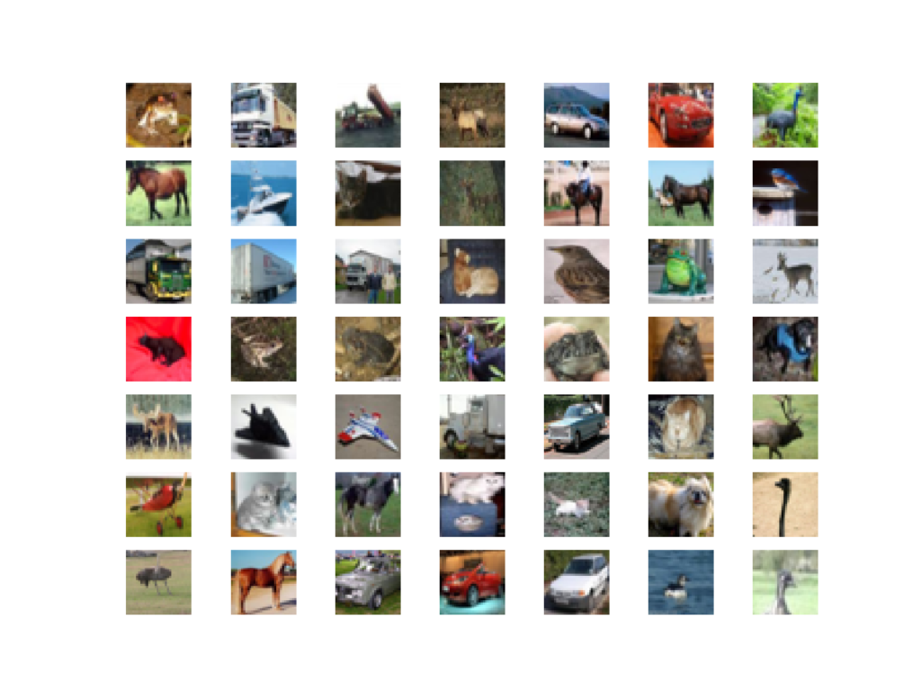
Running the example creates a figure with a plot of 49 images from the CIFAR10 training dataset, arranged in a 7×7 square.
In the plot, you can see small photographs of planes, trucks, horses, cars, frogs, and so on.
Plot of the First 49 Small Object Photographs From the CIFAR10 Dataset.
We will use the images in the training dataset as the basis for training a Generative Adversarial Network.
Specifically, the generator model will learn how to generate new plausible photographs of objects using a discriminator that will try and distinguish between real images from the CIFAR10 training dataset and new images output by the generator model.
This is a non-trivial problem that requires modest generator and discriminator models that are probably most effectively trained on GPU hardware.
For help using cheap Amazon EC2 instances to train deep learning models, see the post:
Take my free 7-day email crash course now (with sample code).
Click to sign-up and also get a free PDF Ebook version of the course.
How to Define and Train the Discriminator Model
The first step is to define the discriminator model.
The model must take a sample image from our dataset as input and output a classification prediction as to whether the sample is real or fake. This is a binary classification problem.
Inputs: Image with three color channel and 32×32 pixels in size.
Outputs: Binary classification, likelihood the sample is real (or fake).
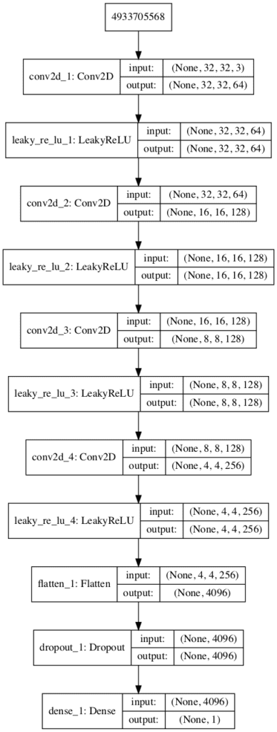
The discriminator model has a normal convolutional layer followed by three convolutional layers using a stride of 2×2 to downsample the input image. The model has no pooling layers and a single node in the output layer with the sigmoid activation function to predict whether the input sample is real or fake. The model is trained to minimize the binary cross entropy loss function, appropriate for binary classification.
Running the example first summarizes the model architecture, showing the input and output from each layer.
We can see that the aggressive 2×2 stride acts to down-sample the input image, first from 32×32 to 16×16, then to 8×8 and more before the model makes an output prediction.
This pattern is by design as we do not use pooling layers and use the large stride to achieve a similar downsampling effect. We will see a similar pattern, but in reverse in the generator model in the next section.
A plot of the model is also created and we can see that the model expects a vector input and will predict a single output.
Note: creating this plot assumes that the pydot and graphviz libraries are installed. If this is a problem, you can comment out the import statement and the call to the plot_model() function.
Plot of the Discriminator Model in the CIFAR10 Generative Adversarial Network
We could start training this model now with real examples with a class label of one and randomly generate samples with a class label of zero.
The development of these elements will be useful later, and it helps to see that the discriminator is just a normal neural network model for binary classification.
First, we need a function to load and prepare the dataset of real images.
We will use the cifar.load_data() function to load the CIFAR-10 dataset and just use the input part of the training dataset as the real images.
1
2
3
...
# load cifar10 dataset
(trainX,_),(_,_)=load_data()
We must scale the pixel values from the range of unsigned integers in [0,255] to the normalized range of [-1,1].
The generator model will generate images with pixel values in the range [-1,1] as it will use the tanh activation function, a best practice.
It is also a good practice for the real images to be scaled to the same range.
1
2
3
4
5
...
# convert from unsigned ints to floats
X=trainX.astype('float32')
# scale from [0,255] to [-1,1]
X=(X-127.5)/127.5
The load_real_samples() function below implements the loading and scaling of real CIFAR-10 photographs.
1
2
3
4
5
6
7
8
9
# load and prepare cifar10 training images
def load_real_samples():
# load cifar10 dataset
(trainX,_),(_,_)=load_data()
# convert from unsigned ints to floats
X=trainX.astype('float32')
# scale from [0,255] to [-1,1]
X=(X-127.5)/127.5
returnX
The model will be updated in batches, specifically with a collection of real samples and a collection of generated samples. On training, an epoch is defined as one pass through the entire training dataset.
We could systematically enumerate all samples in the training dataset, and that is a good approach, but good training via stochastic gradient descent requires that the training dataset be shuffled prior to each epoch. A simpler approach is to select random samples of images from the training dataset.
The generate_real_samples() function below will take the training dataset as an argument and will select a random subsample of images; it will also return class labels for the sample, specifically a class label of 1, to indicate real images.
1
2
3
4
5
6
7
8
9
# select real samples
def generate_real_samples(dataset,n_samples):
# choose random instances
ix=randint(0,dataset.shape[0],n_samples)
# retrieve selected images
X=dataset[ix]
# generate 'real' class labels (1)
y=ones((n_samples,1))
returnX,y
Now, we need a source of fake images.
We don’t have a generator model yet, so instead, we can generate images comprised of random pixel values, specifically random pixel values in the range [0,1], then scaled to the range [-1, 1] like our scaled real images.
The generate_fake_samples() function below implements this behavior and generates images of random pixel values and their associated class label of 0, for fake.
1
2
3
4
5
6
7
8
9
10
11
# generate n fake samples with class labels
def generate_fake_samples(n_samples):
# generate uniform random numbers in [0,1]
X=rand(32*32*3*n_samples)
# update to have the range [-1, 1]
X=-1+X *2
# reshape into a batch of color images
X=X.reshape((n_samples,32,32,3))
# generate 'fake' class labels (0)
y=zeros((n_samples,1))
returnX,y
Finally, we need to train the discriminator model.
This involves repeatedly retrieving samples of real images and samples of generated images and updating the model for a fixed number of iterations.
We will ignore the idea of epochs for now (e.g. complete passes through the training dataset) and fit the discriminator model for a fixed number of batches. The model will learn to discriminate between real and fake (randomly generated) images rapidly, therefore not many batches will be required before it learns to discriminate perfectly.
The train_discriminator() function implements this, using a batch size of 128 images, where 64 are real and 64 are fake each iteration.
We update the discriminator separately for real and fake examples so that we can calculate the accuracy of the model on each sample prior to the update. This gives insight into how the discriminator model is performing over time.
Tying all of this together, the complete example of training an instance of the discriminator model on real and randomly generated (fake) images is listed below.
1
2
3
4
5
6
7
8
9
10
11
12
13
14
15
16
17
18
19
20
21
22
23
24
25
26
27
28
29
30
31
32
33
34
35
36
37
38
39
40
41
42
43
44
45
46
47
48
49
50
51
52
53
54
55
56
57
58
59
60
61
62
63
64
65
66
67
68
69
70
71
72
73
74
75
76
77
78
79
80
81
82
83
84
85
86
87
88
89
90
91
92
93
# example of training the discriminator model on real and random cifar10 images
Running the example first defines the model, loads the CIFAR-10 dataset, then trains the discriminator model.
Note: Your results may vary given the stochastic nature of the algorithm or evaluation procedure, or differences in numerical precision. Consider running the example a few times and compare the average outcome.
In this case, the discriminator model learns to tell the difference between real and randomly generated CIFAR-10 images very quickly, in about 20 batches.
1
2
3
4
5
6
...
>16 real=100% fake=100%
>17 real=100% fake=100%
>18 real=98% fake=100%
>19 real=100% fake=100%
>20 real=100% fake=100%
Now that we know how to define and train the discriminator model, we need to look at developing the generator model.
How to Define and Use the Generator Model
The generator model is responsible for creating new, fake, but plausible small photographs of objects.
It does this by taking a point from the latent space as input and outputting a square color image.
The latent space is an arbitrarily defined vector space of Gaussian-distributed values, e.g. 100 dimensions. It has no meaning, but by drawing points from this space randomly and providing them to the generator model during training, the generator model will assign meaning to the latent points and, in turn, the latent space, until, at the end of training, the latent vector space represents a compressed representation of the output space, CIFAR-10 images, that only the generator knows how to turn into plausible CIFAR-10 images.
Inputs: Point in latent space, e.g. a 100-element vector of Gaussian random numbers.
Outputs: Two-dimensional square color image (3 channels) of 32 x 32 pixels with pixel values in [-1,1].
Note: we don’t have to use a 100 element vector as input; it is a round number and widely used, but I would expect that 10, 50, or 500 would work just as well.
Developing a generator model requires that we transform a vector from the latent space with, 100 dimensions to a 2D array with 32 x 32 x 3, or 3,072 values.
There are a number of ways to achieve this, but there is one approach that has proven effective on deep convolutional generative adversarial networks. It involves two main elements.
The first is a Dense layer as the first hidden layer that has enough nodes to represent a low-resolution version of the output image. Specifically, an image half the size (one quarter the area) of the output image would be 16x16x3, or 768 nodes, and an image one quarter the size (one eighth the area) would be 8 x 8 x 3, or 192 nodes.
With some experimentation, I have found that a smaller low-resolution version of the image works better. Therefore, we will use 4 x 4 x 3, or 48 nodes.
We don’t just want one low-resolution version of the image; we want many parallel versions or interpretations of the input. This is a pattern in convolutional neural networks where we have many parallel filters resulting in multiple parallel activation maps, called feature maps, with different interpretations of the input. We want the same thing in reverse: many parallel versions of our output with different learned features that can be collapsed in the output layer into a final image. The model needs space to invent, create, or generate.
Therefore, the first hidden layer, the Dense, needs enough nodes for multiple versions of our output image, such as 256.
1
2
3
4
# foundation for 4x4 image
n_nodes=256*4*4
model.add(Dense(n_nodes,input_dim=latent_dim))
model.add(LeakyReLU(alpha=0.2))
The activations from these nodes can then be reshaped into something image-like to pass into a convolutional layer, such as 256 different 4 x 4 feature maps.
1
model.add(Reshape((4,4,256)))
The next major architectural innovation involves upsampling the low-resolution image to a higher resolution version of the image.
There are two common ways to do this upsampling process, sometimes called deconvolution.
One way is to use an UpSampling2D layer (like a reverse pooling layer) followed by a normal Conv2D layer. The other and perhaps more modern way is to combine these two operations into a single layer, called a Conv2DTranspose. We will use this latter approach for our generator.
The Conv2DTranspose layer can be configured with a stride of (2×2) that will quadruple the area of the input feature maps (double their width and height dimensions). It is also good practice to use a kernel size that is a factor of the stride (e.g. double) to avoid a checkerboard pattern that can sometimes be observed when upsampling.
This can be repeated two more times to arrive at our required 32 x 32 output image.
Again, we will use the LeakyReLU with a default slope of 0.2, reported as a best practice when training GAN models.
The output layer of the model is a Conv2D with three filters for the three required channels and a kernel size of 3×3 and ‘same‘ padding, designed to create a single feature map and preserve its dimensions at 32 x 32 x 3 pixels. A tanh activation is used to ensure output values are in the desired range of [-1,1], a current best practice.
The define_generator() function below implements this and defines the generator model.
Note: the generator model is not compiled and does not specify a loss function or optimization algorithm. This is because the generator is not trained directly. We will learn more about this in the next section.
Running the example summarizes the layers of the model and their output shape.
We can see that, as designed, the first hidden layer has 4,096 parameters or 256 x 4 x 4, the activations of which are reshaped into 256 4 x 4 feature maps. The feature maps are then upscaled via the three Conv2DTranspose layers to the desired output shape of 32 x 32, until the output layer where three filter maps (channels) are created.
A plot of the model is also created and we can see that the model expects a 100-element point from the latent space as input and will predict a two-element vector as output.
Note: creating this plot assumes that the pydot and graphviz libraries are installed. If this is a problem, you can comment out the import statement and the call to the plot_model() function.
Plot of the Generator Model in the CIFAR-10 Generative Adversarial Network
This model cannot do much at the moment.
Nevertheless, we can demonstrate how to use it to generate samples. This is a helpful demonstration to understand the generator as just another model, and some of these elements will be useful later.
The first step is to generate new points in the latent space. We can achieve this by calling the randn() NumPy function for generating arrays of random numbers drawn from a standard Gaussian.
The array of random numbers can then be reshaped into samples, that is n rows with 100 elements per row. The generate_latent_points() function below implements this and generates the desired number of points in the latent space that can be used as input to the generator model.
1
2
3
4
5
6
7
# generate points in latent space as input for the generator
def generate_latent_points(latent_dim,n_samples):
# generate points in the latent space
x_input=randn(latent_dim *n_samples)
# reshape into a batch of inputs for the network
x_input=x_input.reshape(n_samples,latent_dim)
returnx_input
Next, we can use the generated points as input to the generator model to generate new samples, then plot the samples.
We can update the generate_fake_samples() function from the previous section to take the generator model as an argument and use it to generate the desired number of samples by first calling the generate_latent_points() function to generate the required number of points in latent space as input to the model.
The updated generate_fake_samples() function is listed below and returns both the generated samples and the associated class labels.
1
2
3
4
5
6
7
8
9
# use the generator to generate n fake examples, with class labels
Running the example generates 49 examples of fake CIFAR-10 images and visualizes them on a single plot of 7 by 7 images.
As the model is not trained, the generated images are completely random pixel values in [-1, 1], rescaled to [0, 1]. As we might expect, the images look like a mess of gray.
Example of 49 CIFAR-10 Images Output by the Untrained Generator Model
Now that we know how to define and use the generator model, the next step is to train the model.
How to Train the Generator Model
The weights in the generator model are updated based on the performance of the discriminator model.
When the discriminator is good at detecting fake samples, the generator is updated more, and when the discriminator model is relatively poor or confused when detecting fake samples, the generator model is updated less.
This defines the zero-sum or adversarial relationship between these two models.
There may be many ways to implement this using the Keras API, but perhaps the simplest approach is to create a new model that combines the generator and discriminator models.
Specifically, a new GAN model can be defined that stacks the generator and discriminator such that the generator receives as input random points in the latent space and generates samples that are fed into the discriminator model directly, classified, and the output of this larger model can be used to update the model weights of the generator.
To be clear, we are not talking about a new third model, just a new logical model that uses the already-defined layers and weights from the standalone generator and discriminator models.
Only the discriminator is concerned with distinguishing between real and fake examples, therefore the discriminator model can be trained in a standalone manner on examples of each, as we did in the section on the discriminator model above.
The generator model is only concerned with the discriminator’s performance on fake examples. Therefore, we will mark all of the layers in the discriminator as not trainable when it is part of the GAN model so that they can not be updated and overtrained on fake examples.
When training the generator via this logical GAN model, there is one more important change. We want the discriminator to think that the samples output by the generator are real, not fake. Therefore, when the generator is trained as part of the GAN model, we will mark the generated samples as real (class 1).
Why would we want to do this?
We can imagine that the discriminator will then classify the generated samples as not real (class 0) or a low probability of being real (0.3 or 0.5). The backpropagation process used to update the model weights will see this as a large error and will update the model weights (i.e. only the weights in the generator) to correct for this error, in turn making the generator better at generating good fake samples.
Let’s make this concrete.
Inputs: Point in latent space, e.g. a 100-element vector of Gaussian random numbers.
Outputs: Binary classification, likelihood the sample is real (or fake).
The define_gan() function below takes as arguments the already-defined generator and discriminator models and creates the new, logical third model subsuming these two models. The weights in the discriminator are marked as not trainable, which only affects the weights as seen by the GAN model and not the standalone discriminator model.
The GAN model then uses the same binary cross entropy loss function as the discriminator and the efficient Adam version of stochastic gradient descent with the learning rate of 0.0002 and momentum of 0.5, recommended when training deep convolutional GANs.
1
2
3
4
5
6
7
8
9
10
11
12
13
14
# define the combined generator and discriminator model, for updating the generator
Making the discriminator not trainable is a clever trick in the Keras API.
The trainable property impacts the model after it is compiled. The discriminator model was compiled with trainable layers, therefore the model weights in those layers will be updated when the standalone model is updated via calls to the train_on_batch() function.
The discriminator model was then marked as not trainable, added to the GAN model, and compiled. In this model, the model weights of the discriminator model are not trainable and cannot be changed when the GAN model is updated via calls to the train_on_batch() function. This change in the trainable property does not impact the training of the standalone discriminator model.
This behavior is described in the Keras API documentation here:
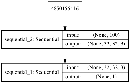
A plot of the model is also created and we can see that the model expects a 100-element point in latent space as input and will predict a single output classification label.
Note: creating this plot assumes that the pydot and graphviz libraries are installed. If this is a problem, you can comment out the import statement and the call to the plot_model() function.
Plot of the Composite Generator and Discriminator Model in the CIFAR-10 Generative Adversarial Network
Training the composite model involves generating a batch worth of points in the latent space via the generate_latent_points() function in the previous section, and class=1 labels and calling the train_on_batch() function.
The train_gan() function below demonstrates this, although it is pretty simple as only the generator will be updated each epoch, leaving the discriminator with default model weights.
# prepare points in latent space as input for the generator
x_gan=generate_latent_points(latent_dim,n_batch)
# create inverted labels for the fake samples
y_gan=ones((n_batch,1))
# update the generator via the discriminator's error
gan_model.train_on_batch(x_gan,y_gan)
Instead, what is required is that we first update the discriminator model with real and fake samples, then update the generator via the composite model.
This requires combining elements from the train_discriminator() function defined in the discriminator section above and the train_gan() function defined above. It also requires that we enumerate over both epochs and batches within in an epoch.
The complete train function for updating the discriminator model and the generator (via the composite model) is listed below.
There are a few things to note in this model training function.
First, the number of batches within an epoch is defined by how many times the batch size divides into the training dataset. We have a dataset size of 50K samples, so with rounding down, there are 390 batches per epoch.
The discriminator model is updated twice per batch, once with real samples and once with fake samples, which is a best practice as opposed to combining the samples and performing a single update.
Finally, we report the loss each batch. It is critical to keep an eye on the loss over batches. The reason for this is that a crash in the discriminator loss indicates that the generator model has started generating rubbish examples that the discriminator can easily discriminate.
Monitor the discriminator loss and expect it to hover around 0.5 to 0.8 per batch. The generator loss is less critical and may hover between 0.5 and 2 or higher. A clever programmer might even attempt to detect the crashing loss of the discriminator, halt, and then restart the training process.
# prepare points in latent space as input for the generator
X_gan=generate_latent_points(latent_dim,n_batch)
# create inverted labels for the fake samples
y_gan=ones((n_batch,1))
# update the generator via the discriminator's error
g_loss=gan_model.train_on_batch(X_gan,y_gan)
# summarize loss on this batch
print('>%d, %d/%d, d1=%.3f, d2=%.3f g=%.3f'%
(i+1,j+1,bat_per_epo,d_loss1,d_loss2,g_loss))
We almost have everything we need to develop a GAN for the CIFAR-10 photographs of objects dataset.
One remaining aspect is the evaluation of the model.
How to Evaluate GAN Model Performance
Generally, there are no objective ways to evaluate the performance of a GAN model.
We cannot calculate this objective error score for generated images.
Instead, images must be subjectively evaluated for quality by a human operator. This means that we cannot know when to stop training without looking at examples of generated images. In turn, the adversarial nature of the training process means that the generator is changing after every batch, meaning that once “good enough” images can be generated, the subjective quality of the images may then begin to vary, improve, or even degrade with subsequent updates.
There are three ways to handle this complex training situation.
Periodically evaluate the classification accuracy of the discriminator on real and fake images.
Periodically generate many images and save them to file for subjective review.
Periodically save the generator model.
All three of these actions can be performed at the same time for a given training epoch, such as every 10 training epochs. The result will be a saved generator model for which we have a way of subjectively assessing the quality of its output and objectively knowing how well the discriminator was fooled at the time the model was saved.
Training the GAN over many epochs, such as hundreds or thousands of epochs, will result in many snapshots of the model that can be inspected, and from which specific outputs and models can be cherry-picked for later use.
First, we can define a function called summarize_performance() that will summarize the performance of the discriminator model. It does this by retrieving a sample of real CIFAR-10 images, as well as generating the same number of fake CIFAR-10 images with the generator model, then evaluating the classification accuracy of the discriminator model on each sample, and reporting these scores.
1
2
3
4
5
6
7
8
9
10
11
12
# evaluate the discriminator, plot generated images, save generator model
Next, we can update the summarize_performance() function to both save the model and to create and save a plot generated examples.
The generator model can be saved by calling the save() function on the generator model and providing a unique filename based on the training epoch number.
1
2
3
4
...
# save the generator model tile file
filename='generator_model_%03d.h5'%(epoch+1)
g_model.save(filename)
We can develop a function to create a plot of the generated samples.
As we are evaluating the discriminator on 100 generated CIFAR-10 images, we can plot about half, or 49, as a 7 by 7 grid. The save_plot() function below implements this, again saving the resulting plot with a unique filename based on the epoch number.
1
2
3
4
5
6
7
8
9
10
11
12
13
14
15
16
# create and save a plot of generated images
def save_plot(examples,epoch,n=7):
# scale from [-1,1] to [0,1]
examples=(examples+1)/2.0
# plot images
foriinrange(n *n):
# define subplot
pyplot.subplot(n,n,1+i)
# turn off axis
pyplot.axis('off')
# plot raw pixel data
pyplot.imshow(examples[i])
# save plot to file
filename='generated_plot_e%03d.png'%(epoch+1)
pyplot.savefig(filename)
pyplot.close()
The updated summarize_performance() function with these additions is listed below.
1
2
3
4
5
6
7
8
9
10
11
12
13
14
15
16
17
# evaluate the discriminator, plot generated images, save generator model
We now have everything we need to train and evaluate a GAN on the CIFAR-10 photographs of small objects dataset.
The complete example is listed below.
Note: this example can run on a CPU but may take a number of hours. The example can run on a GPU, such as the Amazon EC2 p3 instances, and will complete in a few minutes.
For help on setting up an AWS EC2 instance to run this code, see the tutorial:
The chosen configuration results in the stable training of both the generative and discriminative model.
The model performance is reported every batch, including the loss of both the discriminative (d) and generative (g) models.
Note: Your results may vary given the stochastic nature of the algorithm or evaluation procedure, or differences in numerical precision. Consider running the example a few times and compare the average outcome.
In this case, the loss remains stable over the course of training. The discriminator loss on the real and generated examples sits around 0.5, whereas the loss for the generator trained via the discriminator sits around 1.5 for much of the training process.
1
2
3
4
5
6
7
8
9
10
11
>1, 1/390, d1=0.720, d2=0.695 g=0.692
>1, 2/390, d1=0.658, d2=0.697 g=0.691
>1, 3/390, d1=0.604, d2=0.700 g=0.687
>1, 4/390, d1=0.522, d2=0.709 g=0.680
>1, 5/390, d1=0.417, d2=0.731 g=0.662
...
>200, 386/390, d1=0.499, d2=0.401 g=1.565
>200, 387/390, d1=0.459, d2=0.623 g=1.481
>200, 388/390, d1=0.588, d2=0.556 g=1.700
>200, 389/390, d1=0.579, d2=0.288 g=1.555
>200, 390/390, d1=0.620, d2=0.453 g=1.466
The generator is evaluated every 10 epochs, resulting in 20 evaluations, 20 plots of generated images, and 20 saved models.
In this case, we can see that the accuracy fluctuates over training. When viewing the discriminator model’s accuracy score in concert with generated images, we can see that the accuracy on fake examples does not correlate well with the subjective quality of images, but the accuracy for real examples may.
It is a crude and possibly unreliable metric of GAN performance, along with loss.
1
2
3
4
5
6
>Accuracy real: 55%, fake: 89%
>Accuracy real: 50%, fake: 75%
>Accuracy real: 49%, fake: 86%
>Accuracy real: 60%, fake: 79%
>Accuracy real: 49%, fake: 87%
...
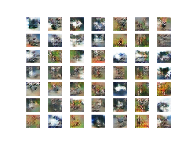
More training, beyond some point, does not mean better quality generated images.
In this case, the results after 10 epochs are low quality, although we can see some difference between background and foreground with a blog in the middle of each image.
Plot of 49 GAN Generated CIFAR-10 Photographs After 10 Epochs
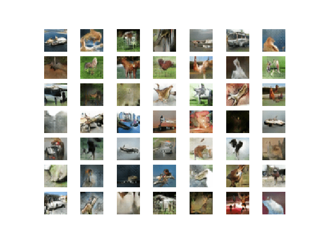
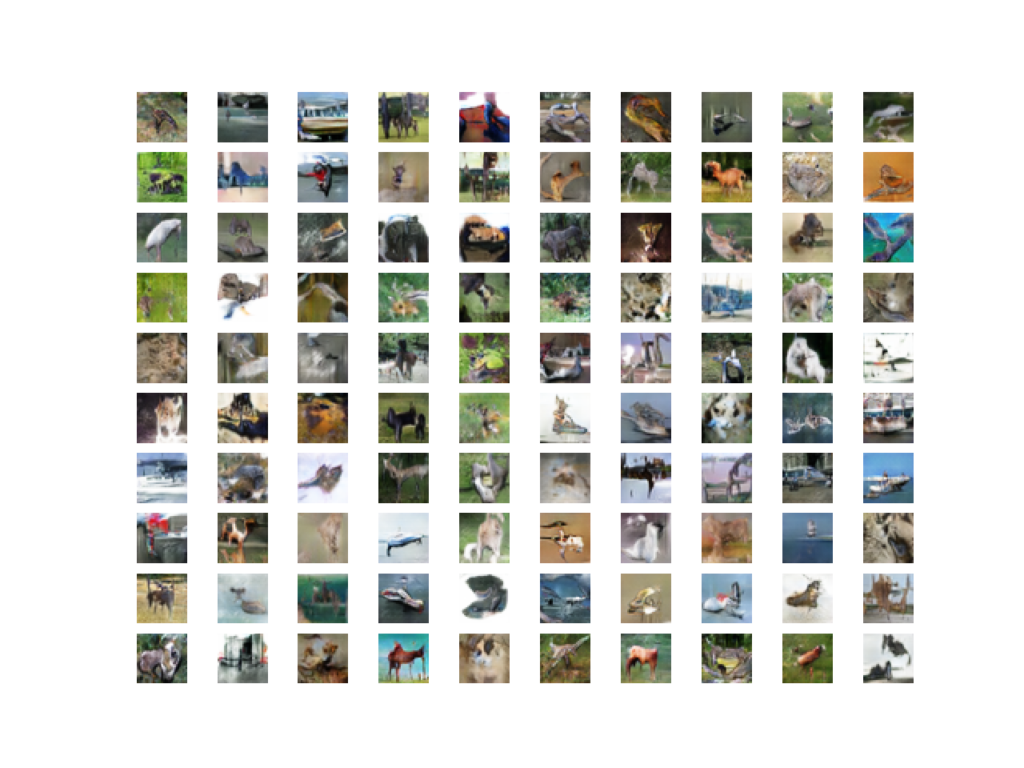
After 90 or 100 epochs, we are starting to see plausible photographs with blobs that look like birds, dogs, cats, and horses.
The objects are familiar and CIFAR-10-like, but many of them are not clearly one of the 10 specified classes.
Plot of 49 GAN Generated CIFAR-10 Photographs After 90 Epochs
Plot of 49 GAN Generated CIFAR-10 Photographs After 100 Epochs
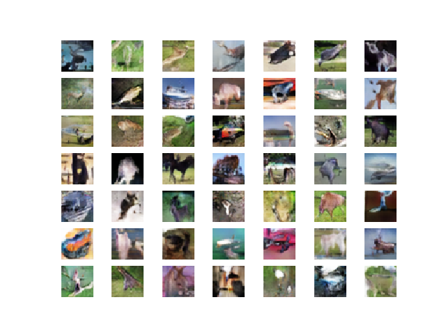
The model remains stable over the next 100 epochs, with little major improvement in the generated images.
The small photos remain vaguely CIFAR-10 like and focused on animals like dogs, cats, and birds.
Plot of 49 GAN Generated CIFAR-10 Photographs After 200 Epochs
How to Use the Final Generator Model to Generate Images
Once a final generator model is selected, it can be used in a standalone manner for your application.
This involves first loading the model from file, then using it to generate images. The generation of each image requires a point in the latent space as input.
The complete example of loading the saved model and generating images is listed below. In this case, we will use the model saved after 200 training epochs, but the model saved after 100 epochs would work just as well.
1
2
3
4
5
6
7
8
9
10
11
12
13
14
15
16
17
18
19
20
21
22
23
24
25
26
27
28
29
30
31
32
33
34
35
# example of loading the generator model and generating images
from keras.models import load_model
from numpy.random import randn
from matplotlib import pyplot
# generate points in latent space as input for the generator
def generate_latent_points(latent_dim,n_samples):
# generate points in the latent space
x_input=randn(latent_dim *n_samples)
# reshape into a batch of inputs for the network
x_input=x_input.reshape(n_samples,latent_dim)
returnx_input
# plot the generated images
def create_plot(examples,n):
# plot images
foriinrange(n *n):
# define subplot
pyplot.subplot(n,n,1+i)
# turn off axis
pyplot.axis('off')
# plot raw pixel data
pyplot.imshow(examples[i,:,:])
pyplot.show()
# load model
model=load_model('generator_model_200.h5')
# generate images
latent_points=generate_latent_points(100,100)
# generate images
X=model.predict(latent_points)
# scale from [-1,1] to [0,1]
X=(X+1)/2.0
# plot the result
create_plot(X,10)
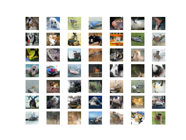
Running the example first loads the model, samples 100 random points in the latent space, generates 100 images, then plots the results as a single image.
Note: Your results may vary given the stochastic nature of the algorithm or evaluation procedure, or differences in numerical precision. Consider running the example a few times and compare the average outcome.
We can see that most of the images are plausible, or plausible pieces of small objects.
I can see dogs, cats, horses, birds, frogs, and perhaps planes.
Example of 100 GAN Generated CIFAR-10 Small Object Photographs
The latent space now defines a compressed representation of CIFAR-10 photos.
You can experiment with generating different points in this space and see what types of images they generate.
The example below generates a single image using a vector of all 0.75 values.
1
2
3
4
5
6
7
8
9
10
11
12
13
14
15
# example of generating an image for a specific point in the latent space
from keras.models import load_model
from numpy import asarray
from matplotlib import pyplot
# load model
model=load_model('generator_model_200.h5')
# all 0s
vector=asarray([[0.75for_inrange(100)]])
# generate image
X=model.predict(vector)
# scale from [-1,1] to [0,1]
X=(X+1)/2.0
# plot the result
pyplot.imshow(X[0,:,:])
pyplot.show()
Note: Your results may vary given the stochastic nature of the algorithm or evaluation procedure, or differences in numerical precision. Consider running the example a few times and compare the average outcome.
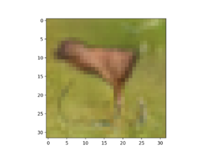
In this case, a vector of all 0.75 results in a deer or perhaps deer-horse-looking animal in a green field.
Example of a GAN Generated CIFAR Small Object Photo for a Specific Point in the Latent Space
Extensions
This section lists some ideas for extending the tutorial that you may wish to explore.
Change Latent Space. Update the example to use a larger or smaller latent space and compare the quality of the results and speed of training.
Batch Normalization. Update the discriminator and/or the generator to make use of batch normalization, recommended for DCGAN models.
Label Smoothing. Update the example to use one-sided label smoothing when training the discriminator, specifically change the target label of real examples from 1.0 to 0.9 and add random noise, then review the effects on image quality and speed of training.
Model Configuration. Update the model configuration to use deeper or more shallow discriminator and/or generator models, perhaps experiment with the UpSampling2D layers in the generator.
If you explore any of these extensions, I’d love to know.
Post your findings in the comments below.
Further Reading
This section provides more resources on the topic if you are looking to go deeper.
Posts
Chapter 20. Deep Generative Models, Deep Learning, 2016.
In this tutorial, you discovered how to develop a generative adversarial network with deep convolutional networks for generating small photographs of objects.
Specifically, you learned:
How to define and train the standalone discriminator model for learning the difference between real and fake images.
How to define the standalone generator model and train the composite generator and discriminator model.
How to evaluate the performance of the GAN and use the final standalone generator model to generate new images.
Do you have any questions?
Ask your questions in the comments below and I will do my best to answer.
Hello! Thanks for your work. I did GAN in pytorch, tensorflow, but they are not so good in GAN. But your work opened up Keras to me. I’m taking your code for my AI, I’ll improve it. Thank you very much.
Jason, thanks much for all your tutorials. Really appreciate the work you put in to explain concepts and has really helped me to understand some of these really complicated things.
Quick question on this, can the above code be used on images of higher resolution as well by simply changing the input and output dimensions from 32x32x3 to a higher value and changing how you upsampled/downsampled things, or basically are there any other tricks involved.
and is this pretty much how deep fake is implemented as well.
I used this tutorial to learn how to implement GANS. I’ve hacked about with the code and programmed the same topology of Robbie Barrat’s art DCGAN (the one that generated the portrait that sold for $432,500 at Christie’s)
It allows you to load your own dataset of 128×128 RGB images
Jason, after displaying the discriminator model, you refer to it saying “A plot of the model is also created and we can see that the model expects two inputs and will predict a single output.” I think this text could have been contaminated by some other text and you really wanted to write “one input”. I only tell you because I know you are a perfectionist, so may be you wanted to correct it (I like what you write anyway).
Dr. Vimal ShrivastavaFebruary 21, 2020 at 2:39 pm#
Thanks for sharing a detailed discussion on GAN.I have a query that is it possible to get the class label of the generated images through code?
How can we do that.
Jason, I like a lot (a lot), your pedagogical approach. You are not afraid to repeat pieces of code, even if there are slight changes which the reader could infer. You display it again, leaving the focus of the reader on the content; so he or she is not distracted by the need to fill the gaps. There are no gaps in what you write and a reader can follow the flow of reasoning with no disruption (I love when you write “the complete example is…”, “let’s tight everything together…”). Yes, we could compile the pieces of codes ourselves, but now we are concentrated in getting to the end of the story and you keep us on track. Moreover, often the “compilation” it is not obvious to the new reader and it is a fun exercise to verify, off-line, the single components. Seeing many times the same code with the consistency of the naming conventions and descriptions that you ensure across different tutorials results in a kind of supervised learning for the user which is presented with augmented examples; it works. This is Fantastic!
Your choice to avoid embedding everything into classes also contributes to an easy reading. It could be more “elegant” to build objects, but then it would require the users to find their way through the properties and methods allocated to each different element. You fight unnecessary effort deviating from the Goal and therefore you compact all the required functionalities in clean functions; they will be used by what ever part of the code will need them. In your tutorials you don’t protect or hide, you clearly favor visibility.
I have seen many effective examples and tutorials in the internet, but rarely, such as in your writing, I have found your extraordinary effort to make sure that the reader actually learns, the continuous pressing on key items (seen from different angles) to reinforce the learning. This is a recognition to the instructor skills as instructor. I am sure it represents the view of your readers.
Back to work.
In # example of loading the generator model and generating images
you are naturally reusing # create and save a plot of generated images
overriding the previous function. However, this time you are not saving the image as you are really displaying it with pyplot.show(). Without needing to change the name of save_plot() may be you could change the comment # create and save a plot of generated images to
# create and show a plot of generated images. Unless you want to interpret Savings as Save to screen.
You might be the first to really and deeply notice my “style” after all these years of writing. Thank you for noticing and appreciating. Yes, it is intentional to use consistent naming conventions, to use repetition, to design the articles with pieces leading up to a complete example and to not use classes and more fancy APIs. I’m happy that it is helping.
Thanks for the note re the code, I have updated the example to be clearer.
I strongly agree with Antonio. You are a talented teacher (I am a professor at a Parisian university in France, and I feel very humbled by your talent. I use many of your examples in my course (with a link to your blog) and I insist on your pedagogical approach.
Many thanks, once again
Thanks a lot for a wonderful tutorial.
I pretty much understood that we trained discriminator on standalone fashion and then made its weights not-trainable. Then designed generator model which fed its output into a trained discriminator. We could have then trained this combined model to update weights of just the generator and finish the job. We could have then used just the generator part to create new photos.
In this scenario (combined model as above) I am not able to write a code that would give me intermediate layer output. That is output of what generator part generates in 32x32x3 dimension.
This eventually gets fed into discriminator but I wanted to capture it before that happens and see how photos look. How to achieve this? Keras “Model” definition is not helping either.
In tutorial we changed strategy to combine generator and discriminator and train them together in cycles. Why was this?
Perhaps you can design the composite model to have 2 outputs, one from the generator and one from the discriminator. Should be easy with the functional API.
Hi, Jason, thank you for the great post ! I’m following your articles for a whilte. these are really specific and easy to understand.
So, one question, I’m still consufed about how generator updates it’s weights based on the gan’s loss. for my better understanding, let me put your defining gan part code here:
def define_gan(g_model, d_model):
# make weights in the discriminator not trainable
d_model.trainable = False
# connect them
model = Sequential()
# add generator
model.add(g_model)
# add the discriminator
model.add(d_model)
# compile model
opt = Adam(lr=0.0002, beta_1=0.5)
model.compile(loss=’binary_crossentropy’, optimizer=opt)
return model
so, in this part, you said we will freeze d_models weights to prevent from update, and will let d_model to think the output of g_model is real (class 1). let’s say g_model generates an image, passes it into d_model, and d_model outputs a number, for example 0.6, but real should be 1.0, which produces a loss (mayby I am thinking this too simple), but how extactly generator model updates it’s weights to ‘real’ direction, how doe’s it know what it the ‘real’ direction ?
Hi! Would just first like to say thank you for making this (and so many other tutorials on machine learning)! Anyway, i would like to know if after saving the discriminative and generative model, is there a way to general both a new image TOGETHER with its 10-class class label? I believe in your example, only the images were generated without the 10-class label. (In your generate fake samples function the y were all zeros). Thanks alot again!
Thanks a lot for your tutorials!!
I have tried to implement a GAN for only the first class in the CIFAR10 dataset, the airplanes. I display the images generated after each epoch, and after running around 100 epochs the generated images are still black and white. Is there something in particular I am doing wrong, or has misunderstood?
Really hope you could have the time to answer this question.
Can I apply this algorithm on a small dataset to produce more images? I only have 30 samples for each class. So I’m looking for a way to expand my dataset.
I have a question. According to this tutorial we have trained the discriminator model beforehand on random noise data and then using this model to classify the generator model as fake but my question is that wouldn’t it be beneficial to train the model on the go with the fake outputs from the generator because then the discriminator model will have a hard time identifying the fake images from the true ones as the generator model is also learning simultaneously and thus both are getting better and thus achieving better result or is my theory flawed.
Q. Inside the train function, we are already passing the gan_model hence the model will not change. Inside the gan_model we have the initial discriminator function that has not been trained and is not trainable as per the define_gan(). How will the discriminator training in the train function change the weights of the discriminator function if the gan model already passed is locked on discriminator?
So when the discriminator is trained for that batch, it does update the gan_model but when the gan model is trained the discriminator remains untouched. Am I interpretting it correctly?
So as the training of the GAN goes on, the generator will get better at creating images. So at that time when we feed the fake samples generated from generator into the discriminator, those will be very close to real images. And if we label them with 0 then the discriminator will be trained to detect these samples as fake which is not what we want. It will be trained to classify these “kind of real images” generated by the generator as fake
I had followed along the tutorial and implemented the code but my d_loss_1 and d_loss_2 seem to become very small after the first train batch (around 0.0023) and so does my gan_loss (around 0.002). This is not producing the desired results. I checked the whole code 10 times and could not find any difference or discrepancy. Could you help me in some way?
Thanks for the reply Jason. I figured it out. It was the batch normalization layers that were causing the problem. But I wonder why it could cause a problem ? With batch norm the weights get learned faster and therefore the error was quite low but I am not really sure why the generated images were not upto the mark
Hi, I am using batch Normalization layers and all my images are just random noise no matter how long i train for? if i remove the Batch normalization it works well. I cant figure out why it is not training with the batch normalization. thank you in advance for any help you can give.
hi this is very helpful tutorial. I am new to this field. I tried running it but after training, It didn’t come up with any images. it just shows accuracy of fake and real. i wonder why?
i only changed Epochs to 10 as it is very time consuming on CPU and i wanted to see the output. i only need to create 20 images.
I picked up this architecture to train CIFAR-10 using WGAN model. Wonder why am I not able to generate good images? All I am getting is noisy images. Have a look at the loss though. It should generate good quality images accordingly.
Hey
I’m trying to load my own dataset to generate images. It is to perform some kind of voice cloning application, so it is my own dataset containing one label and 3001 images.
when i try to run this model, it gives the error:
TypeError: Required argument ‘mean’ (pos 2) not found
At #
def generate_latent_points(latent_dim, n_samples):
….
Your code help me in understanding the over all flow clearly. I appreciate it. But i have a question and hopefully i can get answer from you.
My question is :
1. I trained my model save my weight of discriminator and GAN right. Now i want to load the model feed the trained weight and want to generate image from my input image. How this can be achieved? because in sample model we just load model, provide weights and call model.predict(input)->.
can you please explain how to handle this in GAN or DCGAN?
Hi, this is a very helpful tutorial, thank you! I was wondering if there any benchmarking libraries in python to use for training and evaluating my GAN. I’ve found many other libraries for other concepts, such as adversarial examples via cleverhans. However I haven’t found anything related specifically to GANs? Any ideas? Thanks again for your help.
Would it not make more sense to consider the performance of a well-trained discriminator as an objective measure of the generator’s performance, instead of the DCGAN’s discriminator’s performance?
I will be given some images, if they are input size, it will give an additional similar image automatically, for example, if I give 10 pictures, 11 pictures will be shown in the output.
How can I salvage it ??
I will input some number of images.my model will automatically give me an image output based on the image given in an input.How to I do this using deep learning ??
Thanks for taking your time writing this tutorial.
Can I ask if you have used multiple GPUs to train GAN? I found it very hard to achieve because GAN actually consists of multiple models which are initiated in different functions. Any suggestions would be highly appreciated.
Hi, I would like to ask about the random number that appears before input dense layers in both two plots of the discriminative model and generative model. Is it a random value? And does it have any meaning?
I received different values when I plot the models, but I don’t really understand it.
Thank you so much.
Hi Jason, I wanna ask if i want to generate diabetic retinopathy fundus image with 256×256 dimension and i have 3 classes to generate which their amount are 20, 70 and 50. I wanted to make them into average 140. Can this GAN able to generate? What setting should i set?
The simplest difference is the number of channels. In black and white, we assume the input/output is a grid of float (e.g., 0 to 1) but for color, you need three grids of float for the RGB channels.
# load and prepare mnist training images
def load_real_samples():
# load mnist dataset
(trainX, _), (_, _) = load_data()
# expand to 3d, e.g. add channels dimension
X = expand_dims(trainX, axis=-1)
# convert from unsigned ints to floats
X = X.astype(‘float32’)
# scale from [0,255] to [0,1]
X = X / 255.0
return X
Thankyou for a great article and model.
I have run the model in Colab, but get the message:
‘WARNING: tensorflow: Compiled the loaded model, but the compiled metrics have yet to be built. model.compile metrics will be empty until you train or evaluate the model.’
Chandra Sekhar VoruguntiMarch 26, 2022 at 3:55 pm#
Hi Jason,
Good Morning,
Before running the “Complete Example of GAN for CIFAR-10”, do we need train the descriminator independently or the “Complete Example of GAN for CIFAR-10” will take care.
Please I ran your exact code without changing anything and I am getting this error:
—————————————————————————
TypeError Traceback (most recent call last)
in
20 dataset = load_real_samples()
21 # fit the model
—> 22 train_discriminator(model, dataset)
in train_discriminator(model, dataset, n_iter, n_batch)
5 for i in range(n_iter):
6 # get randomly selected ‘real’ samples
—-> 7 X_real, y_real = generate_real_samples(dataset, half_batch)
8 # update discriminator on real samples
9 _, real_acc = model.train_on_batch(X_real, y_real)
in generate_real_samples(dataset, n_samples)
2 def generate_real_samples(dataset, n_samples):
3 # choose random instances
—-> 4 ix = randint(0, dataset.shape[0], n_samples)
5 # retrieve selected images
6 X = dataset[ix]
TypeError: randint() takes 3 positional arguments but 4 were given
I want to make a GAN model. But ı have a questıon. How can ı change to gan input vector.(latent space). I want to make different colour palette image. İf ı choose the red palette ı want to red and same colour output.
I have limited dataset(50 samples) and only 2 classes of CIFAR10 (100 images in total). I can’t use more than 50 samples for each class and I’d like to generate fake images of that particular 2 classes images in order to expand my dataset. How can I do that? Thank you.


 From Scratch with Keras")


 From Scratch")
 in Keras")
Hello. Thank you for the post. I can use GAN to classification?
You could use the discriminator for classification or as a starting point for transfer learning.
Hello! Thanks for your work. I did GAN in pytorch, tensorflow, but they are not so good in GAN. But your work opened up Keras to me. I’m taking your code for my AI, I’ll improve it. Thank you very much.
Hi GosSamer…Thank you for your feedback! Let us know how your models perform going foward.
The best GAN tutorial so far. Many thanks!
Thanks!
Jason, thanks much for all your tutorials. Really appreciate the work you put in to explain concepts and has really helped me to understand some of these really complicated things.
Quick question on this, can the above code be used on images of higher resolution as well by simply changing the input and output dimensions from 32x32x3 to a higher value and changing how you upsampled/downsampled things, or basically are there any other tricks involved.
and is this pretty much how deep fake is implemented as well.
Yes, exactly.
Although you may need more fancy tricks to make the model stable:
https://machinelearningmastery.com/how-to-code-generative-adversarial-network-hacks/
Hi,
I used this tutorial to learn how to implement GANS. I’ve hacked about with the code and programmed the same topology of Robbie Barrat’s art DCGAN (the one that generated the portrait that sold for $432,500 at Christie’s)
It allows you to load your own dataset of 128×128 RGB images
check it out here:
https://github.com/jordan-bird/art-DCGAN-Keras
PS: Cheers for the great tutorial, Jason
Very cool Jordan, thanks for sharing!
Thanks so much for the article. Where can i download the dataset? Many thanks!
It is downloaded when you call:
Jason, after displaying the discriminator model, you refer to it saying “A plot of the model is also created and we can see that the model expects two inputs and will predict a single output.” I think this text could have been contaminated by some other text and you really wanted to write “one input”. I only tell you because I know you are a perfectionist, so may be you wanted to correct it (I like what you write anyway).
Thanks, fixed.
Thanks for sharing a detailed discussion on GAN.I have a query that is it possible to get the class label of the generated images through code?
How can we do that.
Thank you once again.
Yes, perhaps use a supervised learning model to classify it, e.g. a pre-trained vgg16 or better.
Jason, I like a lot (a lot), your pedagogical approach. You are not afraid to repeat pieces of code, even if there are slight changes which the reader could infer. You display it again, leaving the focus of the reader on the content; so he or she is not distracted by the need to fill the gaps. There are no gaps in what you write and a reader can follow the flow of reasoning with no disruption (I love when you write “the complete example is…”, “let’s tight everything together…”). Yes, we could compile the pieces of codes ourselves, but now we are concentrated in getting to the end of the story and you keep us on track. Moreover, often the “compilation” it is not obvious to the new reader and it is a fun exercise to verify, off-line, the single components. Seeing many times the same code with the consistency of the naming conventions and descriptions that you ensure across different tutorials results in a kind of supervised learning for the user which is presented with augmented examples; it works. This is Fantastic!
Your choice to avoid embedding everything into classes also contributes to an easy reading. It could be more “elegant” to build objects, but then it would require the users to find their way through the properties and methods allocated to each different element. You fight unnecessary effort deviating from the Goal and therefore you compact all the required functionalities in clean functions; they will be used by what ever part of the code will need them. In your tutorials you don’t protect or hide, you clearly favor visibility.
I have seen many effective examples and tutorials in the internet, but rarely, such as in your writing, I have found your extraordinary effort to make sure that the reader actually learns, the continuous pressing on key items (seen from different angles) to reinforce the learning. This is a recognition to the instructor skills as instructor. I am sure it represents the view of your readers.
Back to work.
In # example of loading the generator model and generating images
you are naturally reusing # create and save a plot of generated images
overriding the previous function. However, this time you are not saving the image as you are really displaying it with pyplot.show(). Without needing to change the name of save_plot() may be you could change the comment # create and save a plot of generated images to
# create and show a plot of generated images. Unless you want to interpret Savings as Save to screen.
Thank you Antonio, very kind of you to say.
You might be the first to really and deeply notice my “style” after all these years of writing. Thank you for noticing and appreciating. Yes, it is intentional to use consistent naming conventions, to use repetition, to design the articles with pieces leading up to a complete example and to not use classes and more fancy APIs. I’m happy that it is helping.
Thanks for the note re the code, I have updated the example to be clearer.
Hello Jason,
I strongly agree with Antonio. You are a talented teacher (I am a professor at a Parisian university in France, and I feel very humbled by your talent. I use many of your examples in my course (with a link to your blog) and I insist on your pedagogical approach.
Many thanks, once again
Thanks, that is kind of you to say. I’m happy my exampels are helpful!
Thanks a lot for a wonderful tutorial.
I pretty much understood that we trained discriminator on standalone fashion and then made its weights not-trainable. Then designed generator model which fed its output into a trained discriminator. We could have then trained this combined model to update weights of just the generator and finish the job. We could have then used just the generator part to create new photos.
In this scenario (combined model as above) I am not able to write a code that would give me intermediate layer output. That is output of what generator part generates in 32x32x3 dimension.
This eventually gets fed into discriminator but I wanted to capture it before that happens and see how photos look. How to achieve this? Keras “Model” definition is not helping either.
In tutorial we changed strategy to combine generator and discriminator and train them together in cycles. Why was this?
Thanks
Rajiv
Thanks, I’m glad it helped!
Perhaps you can design the composite model to have 2 outputs, one from the generator and one from the discriminator. Should be easy with the functional API.
How can i replace CIFAR 10 with image dataset in my PC? Could you please explain?
Thanks in advance.. 🙂
Yes, you can load the images and use them to train a gan, I show how to load images here:
https://machinelearningmastery.com/how-to-load-and-manipulate-images-for-deep-learning-in-python-with-pil-pillow/
Thanks for the reply, but when i load the images as list (trainX[]), it shows the error “list object has noattribute astype”.
Sorry to hear that, I have some suggestions here:
https://machinelearningmastery.com/faq/single-faq/why-does-the-code-in-the-tutorial-not-work-for-me
I solved that. Now how can i save all the generated images to a folder? Could you please help?
Yes, I show how in the above tutorial, see the save_plot() function.
But how to save each single images to a folder??
You could change the code to save each image separately if you wish.
How many images I can save? is there any limitations?
No, only the amount of HDD space you have.
Thanks Jason.
Best tutorial ever… the explanation is really clear and step by step
Now I understand about GAN deeper.
Thank you so much.
Thanks, I’m glad it helped!
Thank you so much for this tutorial. Very well explained
You’re welcome. I’m glad it helped.
Hi, Jason, thank you for the great post ! I’m following your articles for a whilte. these are really specific and easy to understand.
So, one question, I’m still consufed about how generator updates it’s weights based on the gan’s loss. for my better understanding, let me put your defining gan part code here:
def define_gan(g_model, d_model):
# make weights in the discriminator not trainable
d_model.trainable = False
# connect them
model = Sequential()
# add generator
model.add(g_model)
# add the discriminator
model.add(d_model)
# compile model
opt = Adam(lr=0.0002, beta_1=0.5)
model.compile(loss=’binary_crossentropy’, optimizer=opt)
return model
so, in this part, you said we will freeze d_models weights to prevent from update, and will let d_model to think the output of g_model is real (class 1). let’s say g_model generates an image, passes it into d_model, and d_model outputs a number, for example 0.6, but real should be 1.0, which produces a loss (mayby I am thinking this too simple), but how extactly generator model updates it’s weights to ‘real’ direction, how doe’s it know what it the ‘real’ direction ?
Good question.
It is updated to better fool the discriminator.
Hi! Would just first like to say thank you for making this (and so many other tutorials on machine learning)! Anyway, i would like to know if after saving the discriminative and generative model, is there a way to general both a new image TOGETHER with its 10-class class label? I believe in your example, only the images were generated without the 10-class label. (In your generate fake samples function the y were all zeros). Thanks alot again!
Thanks!
This model does not know about labels. You might want to look into the conditional GAN models.
Or you could try using a pre-trained model on the CIFAR dataset to classify images.
Hi Jason,
thank you for the tutorial.
Can you please explain how you came up with:
n_nodes = 256 * 4 * 4?
how does one decide on the number of nodes?
Best regards
There are no reliable heuristics to configure the model. I may have used trial and error or copied a config from a related model.
Hi,
Thanks a lot for your tutorials!!
I have tried to implement a GAN for only the first class in the CIFAR10 dataset, the airplanes. I display the images generated after each epoch, and after running around 100 epochs the generated images are still black and white. Is there something in particular I am doing wrong, or has misunderstood?
Really hope you could have the time to answer this question.
GANs are hard to train, perhaps try different architectures or some of the suggestions here:
https://machinelearningmastery.com/how-to-code-generative-adversarial-network-hacks/
where can i get the generator_model_200.h5 file
You run the code and it is created.
Can I apply this algorithm on a small dataset to produce more images? I only have 30 samples for each class. So I’m looking for a way to expand my dataset.
Yes, although if you are trying to expand your dataset, I would strongly recommend data augmentation instead:
https://machinelearningmastery.com/how-to-configure-image-data-augmentation-when-training-deep-learning-neural-networks/
Best GAN tutorial out there! Thank you so much! Honestly felt like I went from zero to hero with this tutorial!
Thanks!
Well done on your progress!
I have a question. According to this tutorial we have trained the discriminator model beforehand on random noise data and then using this model to classify the generator model as fake but my question is that wouldn’t it be beneficial to train the model on the go with the fake outputs from the generator because then the discriminator model will have a hard time identifying the fake images from the true ones as the generator model is also learning simultaneously and thus both are getting better and thus achieving better result or is my theory flawed.
thankyou
No, we don’t train the model on random noise, we use random noise as input to synthesize new images.
You can learn more about how GANs work in general here:
https://machinelearningmastery.com/start-here/#gans
ok thankyou i get it now there was a gap in my understanding.
thankyou 🙂
I’m happy to hear that, you’re welcome.
Great tutorial Jason! Had a question:
Q. Inside the train function, we are already passing the gan_model hence the model will not change. Inside the gan_model we have the initial discriminator function that has not been trained and is not trainable as per the define_gan(). How will the discriminator training in the train function change the weights of the discriminator function if the gan model already passed is locked on discriminator?
Hence should’nt we train the discriminator first and then define the gan model to train it entirely?
No, they are trained together. This is the whole idea of GANs:
https://machinelearningmastery.com/what-are-generative-adversarial-networks-gans/
The generator is trained via the discriminator is the composite model:
https://machinelearningmastery.com/how-to-code-the-generative-adversarial-network-training-algorithm-and-loss-functions/
So when the discriminator is trained for that batch, it does update the gan_model but when the gan model is trained the discriminator remains untouched. Am I interpretting it correctly?
Is the generator used to generate fake images also getting better as training goes along?
Yes.
Yes.
So as the training of the GAN goes on, the generator will get better at creating images. So at that time when we feed the fake samples generated from generator into the discriminator, those will be very close to real images. And if we label them with 0 then the discriminator will be trained to detect these samples as fake which is not what we want. It will be trained to classify these “kind of real images” generated by the generator as fake
Generally yes, although, we don’t really care about how well the discriminator is at the end, only that it is a good challenge for the generator.
We discard the discriminator and keep the generator.
can you upload the trained model too , because the training requires GPU resources which i dont have right now.
Sorry, I don’t upload/share final models. I focus on teaching readers how to build their own models.
You can access cheap GPUs here:
https://machinelearningmastery.com/develop-evaluate-large-deep-learning-models-keras-amazon-web-services/
Hi Jason.
I had followed along the tutorial and implemented the code but my d_loss_1 and d_loss_2 seem to become very small after the first train batch (around 0.0023) and so does my gan_loss (around 0.002). This is not producing the desired results. I checked the whole code 10 times and could not find any difference or discrepancy. Could you help me in some way?
Perhaps try running the example a few times?
Perhaps try inspecting the generated images during a long run, rather than watching loss?
Thanks for the reply Jason. I figured it out. It was the batch normalization layers that were causing the problem. But I wonder why it could cause a problem ? With batch norm the weights get learned faster and therefore the error was quite low but I am not really sure why the generated images were not upto the mark
I’m happy to hear that.
GANs are very fussy.
Hi, I am using batch Normalization layers and all my images are just random noise no matter how long i train for? if i remove the Batch normalization it works well. I cant figure out why it is not training with the batch normalization. thank you in advance for any help you can give.
Perhaps batch norm layers are not a good fit for the model. It could be that simple.
hi this is very helpful tutorial. I am new to this field. I tried running it but after training, It didn’t come up with any images. it just shows accuracy of fake and real. i wonder why?
i only changed Epochs to 10 as it is very time consuming on CPU and i wanted to see the output. i only need to create 20 images.
Thanks!
You must run the example from the command line, not a notebook or IDE:
https://machinelearningmastery.com/faq/single-faq/why-does-the-code-in-the-tutorial-not-work-for-me
I picked up this architecture to train CIFAR-10 using WGAN model. Wonder why am I not able to generate good images? All I am getting is noisy images. Have a look at the loss though. It should generate good quality images accordingly.
(50000, 32, 32, 3)
0 [D loss: 8.213928] [G loss: 0.000266]
1 [D loss: 7.631218] [G loss: -0.009719]
2 [D loss: 6.827905] [G loss: -0.043795]
3 [D loss: 5.744817] [G loss: -0.128916]
4 [D loss: 4.664616] [G loss: -0.302539]
100 [D loss: -34.882454] [G loss: -1.986118]
1016 [D loss: -13.983415] [G loss: -18.977585]
1170 [D loss: -9.365166] [G loss: -10.809624]
1171 [D loss: -7.520091] [G loss: -6.204955]
1172 [D loss: -8.415616] [G loss: -8.243237]
1195 [D loss: -9.166229] [G loss: -8.273212]
1196 [D loss: -8.356554] [G loss: -8.563138]
1231 [D loss: -8.578263] [G loss: -5.937617]
1232 [D loss: -9.183654] [G loss: -9.121166]
1352 [D loss: -8.893832] [G loss: -9.738533]
1353 [D loss: -9.843869] [G loss: -14.416454]
Perhaps start with the architecture in this tutorial and adapt it to your needs:
https://machinelearningmastery.com/how-to-develop-a-generative-adversarial-network-for-a-cifar-10-small-object-photographs-from-scratch/
Hey
I’m trying to load my own dataset to generate images. It is to perform some kind of voice cloning application, so it is my own dataset containing one label and 3001 images.
when i try to run this model, it gives the error:
TypeError: Required argument ‘mean’ (pos 2) not found
At #
def generate_latent_points(latent_dim, n_samples):
….
x_input = randn(latent_dim * n_samples)
…..
can you help? thank you!
Nevermind, it works now. Terribly sorry to disturb. and thank you so very much for these tutorials.
No problem, happy to hear that.
Sorry to hear that.
Perhaps start with the working example, then slowly adapt it to use your dataset.
Hey. Thank you for the amazing article. I have a small doubt here. Why is downsampling done in the generator?
We do not downsample in the generator, we upsample.
Hi Brownlee,
Your code help me in understanding the over all flow clearly. I appreciate it. But i have a question and hopefully i can get answer from you.
My question is :
1. I trained my model save my weight of discriminator and GAN right. Now i want to load the model feed the trained weight and want to generate image from my input image. How this can be achieved? because in sample model we just load model, provide weights and call model.predict(input)->.
can you please explain how to handle this in GAN or DCGAN?
Thank you
I’m happy to hear that.
The above tutorial shows you exactly how to load the model and generate an image.
Hi, this is a very helpful tutorial, thank you! I was wondering if there any benchmarking libraries in python to use for training and evaluating my GAN. I’ve found many other libraries for other concepts, such as adversarial examples via cleverhans. However I haven’t found anything related specifically to GANs? Any ideas? Thanks again for your help.
Thanks!
This can help you evaluate GAN models:
https://machinelearningmastery.com/how-to-evaluate-generative-adversarial-networks/
Why are you saying “d_model.trainable = false”, in “define_gan”. Is it because we have already trained it .What happens if we don’t make it false?
No, because we don’t want to update the weights of d when updating g.
Would it not make more sense to consider the performance of a well-trained discriminator as an objective measure of the generator’s performance, instead of the DCGAN’s discriminator’s performance?
No, it does not correlated with high quality images.
You can learn more here:
https://machinelearningmastery.com/how-to-evaluate-generative-adversarial-networks/
I will be given some images, if they are input size, it will give an additional similar image automatically, for example, if I give 10 pictures, 11 pictures will be shown in the output.
How can I salvage it ??
Sorry, I don’t understand. Perhaps you could rephrase your question or elaborate?
I will input some number of images.my model will automatically give me an image output based on the image given in an input.How to I do this using deep learning ??
If you want an image as output, this sounds like an image transformation problem, perhaps you can use a GAN like pix2pix:
https://machinelearningmastery.com/a-gentle-introduction-to-pix2pix-generative-adversarial-network/
Hi Jason,
Thanks for taking your time writing this tutorial.
Can I ask if you have used multiple GPUs to train GAN? I found it very hard to achieve because GAN actually consists of multiple models which are initiated in different functions. Any suggestions would be highly appreciated.
Regards,
Hank
I have not, sorry.
Hi, I would like to ask about the random number that appears before input dense layers in both two plots of the discriminative model and generative model. Is it a random value? And does it have any meaning?
I received different values when I plot the models, but I don’t really understand it.
Thank you so much.
Might be a bug in the plot generation code at the time I wrote the tutorial. Does not seem to happen any more.
Hi Jason, I wanna ask if i want to generate diabetic retinopathy fundus image with 256×256 dimension and i have 3 classes to generate which their amount are 20, 70 and 50. I wanted to make them into average 140. Can this GAN able to generate? What setting should i set?
What did you tried?
Hi Jason, I am using your books and tutorials in both during PhD and now in Industry.
I have gone through : https://machinelearningmastery.com/how-to-develop-a-generative-adversarial-network-for-an-mnist-handwritten-digits-from-scratch-in-keras/
to generate black and white images.
The current lecture is on CIFAR colour images. What is the code changes we need to do for black and white , color images.
The simplest difference is the number of channels. In black and white, we assume the input/output is a grid of float (e.g., 0 to 1) but for color, you need three grids of float for the RGB channels.
Hi Jason,
In the above exampe, youe haveused X = (X – 127.5) / 127.5. But in
https://machinelearningmastery.com/how-to-develop-a-generative-adversarial-network-for-an-mnist-handwritten-digits-from-scratch-in-keras/
# load and prepare mnist training images
def load_real_samples():
# load mnist dataset
(trainX, _), (_, _) = load_data()
# expand to 3d, e.g. add channels dimension
X = expand_dims(trainX, axis=-1)
# convert from unsigned ints to floats
X = X.astype(‘float32’)
# scale from [0,255] to [0,1]
X = X / 255.0
return X
you have scaled from 0 to 1 .
Can you specify the reason.
Just a different way of normalization. Should not be much difference after training.
Thankyou for a great article and model.
I have run the model in Colab, but get the message:
‘WARNING: tensorflow: Compiled the loaded model, but the compiled metrics have yet to be built.
model.compile metricswill be empty until you train or evaluate the model.’Please advise.
It seems not a breaking error. It is just a warning. Which line caused this?
Hi Adrian…The following discussion may prove helpful regarding the specific error.
https://stackoverflow.com/questions/67970389/warningtensorflowcompiled-the-loaded-model-but-the-compiled-metrics-have-yet
It may also prove beneficial to establish a local Python environment on your machine. Please see the following tutorial:
https://machinelearningmastery.com/setup-python-environment-machine-learning-deep-learning-anaconda/
I have tried that but still it is showing the same error
WARNING:tensorflow:Compiled the loaded model, but the compiled metrics have yet to be built.
2/2 [==============================] – 0s 10ms/step – loss: 0.4915 – accuracy: 0.7344
2/2 [==============================] – 0s 10ms/step – loss: 0.4705 – accuracy: 0.8438
Acc Real:73.4375% Acc Fake:84.375%
any advice on this
Hi Visvas…This is not an “error”, but rather a warning. Your code is executing properly it seems. The following may help clarify the situation:
https://stackoverflow.com/questions/67970389/warningtensorflowcompiled-the-loaded-model-but-the-compiled-metrics-have-yet
Hi Jason,
Good Morning,
Before running the “Complete Example of GAN for CIFAR-10”, do we need train the descriminator independently or the “Complete Example of GAN for CIFAR-10” will take care.
Hi Jason,
Thanks for your wonderful tutorial.
Please I ran your exact code without changing anything and I am getting this error:
—————————————————————————
TypeError Traceback (most recent call last)
in
20 dataset = load_real_samples()
21 # fit the model
—> 22 train_discriminator(model, dataset)
in train_discriminator(model, dataset, n_iter, n_batch)
5 for i in range(n_iter):
6 # get randomly selected ‘real’ samples
—-> 7 X_real, y_real = generate_real_samples(dataset, half_batch)
8 # update discriminator on real samples
9 _, real_acc = model.train_on_batch(X_real, y_real)
in generate_real_samples(dataset, n_samples)
2 def generate_real_samples(dataset, n_samples):
3 # choose random instances
—-> 4 ix = randint(0, dataset.shape[0], n_samples)
5 # retrieve selected images
6 X = dataset[ix]
TypeError: randint() takes 3 positional arguments but 4 were given
Hi Iffy…Please provide some detail around the following so that we may better assist you:
1. How did you enter your code…copy and paste or did you type it?
2. What Python environment? Google Colab or Anaconda or something else?
I want to make a GAN model. But ı have a questıon. How can ı change to gan input vector.(latent space). I want to make different colour palette image. İf ı choose the red palette ı want to red and same colour output.
Hi fatih…The following may be of interest to you:
https://machinelearningmastery.com/introduction-to-progressive-growing-generative-adversarial-networks/
I have limited dataset(50 samples) and only 2 classes of CIFAR10 (100 images in total). I can’t use more than 50 samples for each class and I’d like to generate fake images of that particular 2 classes images in order to expand my dataset. How can I do that? Thank you.
Hi Andrei…Please elaborate on the issues you are encountering with your model so that we may better assist you.
how to run this code on GPU??
I have all the libraries and have tested them they are working fine.
Hi Jitesh…The following resource may be of interest:
https://machinelearningmastery.com/develop-evaluate-large-deep-learning-models-keras-amazon-web-services/
Also, you may want to try Google Colab with a GPU option:
https://machinelearningmastery.com/google-colab-for-machine-learning-projects/