Generative Adversarial Networks, or GANs, are an architecture for training generative models, such as deep convolutional neural networks for generating images.
Developing a GAN for generating images requires both a discriminator convolutional neural network model for classifying whether a given image is real or generated and a generator model that uses inverse convolutional layers to transform an input to a full two-dimensional image of pixel values.
It can be challenging to understand both how GANs work and how deep convolutional neural network models can be trained in a GAN architecture for image generation. A good starting point for beginners is to practice developing and using GANs on standard image datasets used in the field of computer vision, such as the MNIST handwritten digit dataset. Using small and well-understood datasets means that smaller models can be developed and trained quickly, allowing the focus to be put on the model architecture and image generation process itself.
In this tutorial, you will discover how to develop a generative adversarial network with deep convolutional networks for generating handwritten digits.
After completing this tutorial, you will know:
How to define and train the standalone discriminator model for learning the difference between real and fake images.
How to define the standalone generator model and train the composite generator and discriminator model.
How to evaluate the performance of the GAN and use the final standalone generator model to generate new images.
How to Develop a Generative Adversarial Network for an MNIST Handwritten Digits From Scratch in Keras Photo by jcookfisher, some rights reserved.
Tutorial Overview
This tutorial is divided into seven parts; they are:
MNIST Handwritten Digit Dataset
How to Define and Train the Discriminator Model
How to Define and Use the Generator Model
How to Train the Generator Model
How to Evaluate GAN Model Performance
Complete Example of GAN for MNIST
How to Use the Final Generator Model to Generate Images
MNIST Handwritten Digit Dataset
The MNIST dataset is an acronym that stands for the Modified National Institute of Standards and Technology dataset.
It is a dataset of 70,000 small square 28×28 pixel grayscale images of handwritten single digits between 0 and 9.
The task is to classify a given image of a handwritten digit into one of 10 classes representing integer values from 0 to 9, inclusively.
Keras provides access to the MNIST dataset via the mnist.load_dataset() function. It returns two tuples, one with the input and output elements for the standard training dataset, and another with the input and output elements for the standard test dataset.
The example below loads the dataset and summarizes the shape of the loaded dataset.
Note: the first time you load the dataset, Keras will automatically download a compressed version of the images and save them under your home directory in ~/.keras/datasets/. The download is fast as the dataset is only about eleven megabytes in its compressed form.
1
2
3
4
5
6
7
# example of loading the mnist dataset
from keras.datasets.mnist import load_data
# load the images into memory
(trainX,trainy),(testX,testy)=load_data()
# summarize the shape of the dataset
print('Train',trainX.shape,trainy.shape)
print('Test',testX.shape,testy.shape)
Running the example loads the dataset and prints the shape of the input and output components of the train and test splits of images.
We can see that there are 60K examples in the training set and 10K in the test set and that each image is a square of 28 by 28 pixels.
1
2
Train (60000, 28, 28) (60000,)
Test (10000, 28, 28) (10000,)
The images are grayscale with a black background (0 pixel value) and the handwritten digits in white (pixel values near 255). This means if the images were plotted, they would be mostly black with a white digit in the middle.
We can plot some of the images from the training dataset using the matplotlib library using the imshow() function and specify the color map via the ‘cmap‘ argument as ‘gray‘ to show the pixel values correctly.
1
2
# plot raw pixel data
pyplot.imshow(trainX[i],cmap='gray')
Alternately, the images are easier to review when we reverse the colors and plot the background as white and the handwritten digits in black.
They are easier to view as most of the image is now white with the area of interest in black. This can be achieved using a reverse grayscale color map, as follows:
1
2
# plot raw pixel data
pyplot.imshow(trainX[i],cmap='gray_r')
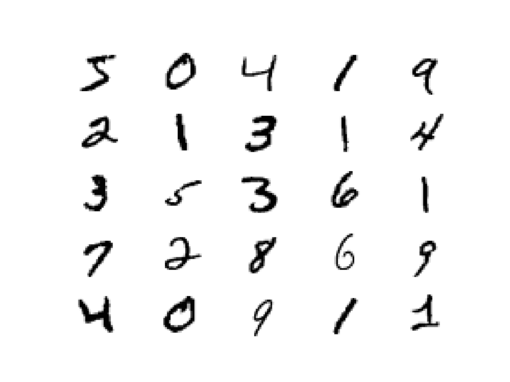
The example below plots the first 25 images from the training dataset in a 5 by 5 square.
1
2
3
4
5
6
7
8
9
10
11
12
13
14
# example of loading the mnist dataset
from keras.datasets.mnist import load_data
from matplotlib import pyplot
# load the images into memory
(trainX,trainy),(testX,testy)=load_data()
# plot images from the training dataset
foriinrange(25):
# define subplot
pyplot.subplot(5,5,1+i)
# turn off axis
pyplot.axis('off')
# plot raw pixel data
pyplot.imshow(trainX[i],cmap='gray_r')
pyplot.show()
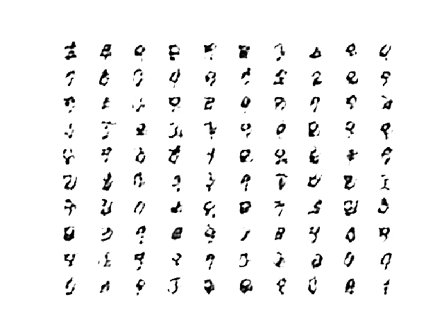
Running the example creates a plot of 25 images from the MNIST training dataset, arranged in a 5×5 square.
Plot of the First 25 Handwritten Digits From the MNIST Dataset.
We will use the images in the training dataset as the basis for training a Generative Adversarial Network.
Specifically, the generator model will learn how to generate new plausible handwritten digits between 0 and 9, using a discriminator that will try to distinguish between real images from the MNIST training dataset and new images output by the generator model.
This is a relatively simple problem that does not require a sophisticated generator or discriminator model, although it does require the generation of a grayscale output image.
Want to Develop GANs from Scratch?
Take my free 7-day email crash course now (with sample code).
Click to sign-up and also get a free PDF Ebook version of the course.
How to Define and Train the Discriminator Model
The first step is to define the discriminator model.
The model must take a sample image from our dataset as input and output a classification prediction as to whether the sample is real or fake.
This is a binary classification problem:
Inputs: Image with one channel and 28×28 pixels in size.
Outputs: Binary classification, likelihood the sample is real (or fake).
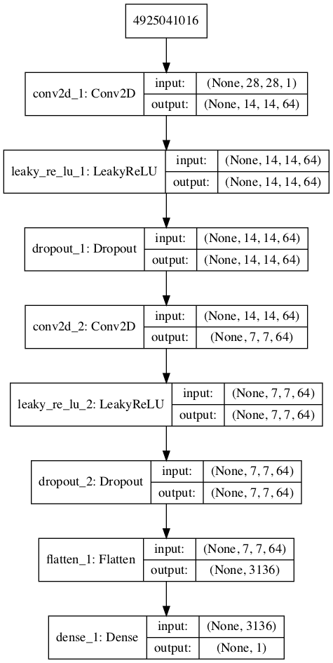
The discriminator model has two convolutional layers with 64 filters each, a small kernel size of 3, and larger than normal stride of 2. The model has no pooling layers and a single node in the output layer with the sigmoid activation function to predict whether the input sample is real or fake. The model is trained to minimize the binary cross entropy loss function, appropriate for binary classification.
We will use some best practices in defining the discriminator model, such as the use of LeakyReLU instead of ReLU, using Dropout, and using the Adam version of stochastic gradient descent with a learning rate of 0.0002 and a momentum of 0.5.
The function define_discriminator() below defines the discriminator model and parametrizes the size of the input image.
This pattern is by design as we do not use pooling layers and use the large stride as achieve a similar downsampling effect. We will see a similar pattern, but in reverse, in the generator model in the next section.
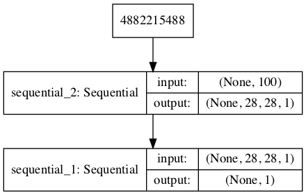
A plot of the model is also created and we can see that the model expects two inputs and will predict a single output.
Note: creating this plot assumes that the pydot and graphviz libraries are installed. If this is a problem, you can comment out the import statement for the plot_model function and the call to the plot_model() function.
Plot of the Discriminator Model in the MNIST GAN
We could start training this model now with real examples with a class label of one, and randomly generated samples with a class label of zero.
The development of these elements will be useful later, and it helps to see that the discriminator is just a normal neural network model for binary classification.
First, we need a function to load and prepare the dataset of real images.
We will use the mnist.load_data() function to load the MNIST dataset and just use the input part of the training dataset as the real images.
1
2
# load mnist dataset
(trainX,_),(_,_)=load_data()
The images are 2D arrays of pixels and convolutional neural networks expect 3D arrays of images as input, where each image has one or more channels.
We must update the images to have an additional dimension for the grayscale channel. We can do this using the expand_dims() NumPy function and specify the final dimension for the channels-last image format.
1
2
# expand to 3d, e.g. add channels dimension
X=expand_dims(trainX,axis=-1)
Finally, we must scale the pixel values from the range of unsigned integers in [0,255] to the normalized range of [0,1].
1
2
3
4
# convert from unsigned ints to floats
X=X.astype('float32')
# scale from [0,255] to [0,1]
X=X/255.0
The load_real_samples() function below implements this.
1
2
3
4
5
6
7
8
9
10
11
# load and prepare mnist training images
def load_real_samples():
# load mnist dataset
(trainX,_),(_,_)=load_data()
# expand to 3d, e.g. add channels dimension
X=expand_dims(trainX,axis=-1)
# convert from unsigned ints to floats
X=X.astype('float32')
# scale from [0,255] to [0,1]
X=X/255.0
returnX
The model will be updated in batches, specifically with a collection of real samples and a collection of generated samples. On training, epoch is defined as one pass through the entire training dataset.
We could systematically enumerate all samples in the training dataset, and that is a good approach, but good training via stochastic gradient descent requires that the training dataset be shuffled prior to each epoch. A simpler approach is to select random samples of images from the training dataset.
The generate_real_samples() function below will take the training dataset as an argument and will select a random subsample of images; it will also return class labels for the sample, specifically a class label of 1, to indicate real images.
1
2
3
4
5
6
7
8
9
# select real samples
def generate_real_samples(dataset,n_samples):
# choose random instances
ix=randint(0,dataset.shape[0],n_samples)
# retrieve selected images
X=dataset[ix]
# generate 'real' class labels (1)
y=ones((n_samples,1))
returnX,y
Now, we need a source of fake images.
We don’t have a generator model yet, so instead, we can generate images comprised of random pixel values, specifically random pixel values in the range [0,1] like our scaled real images.
The generate_fake_samples() function below implements this behavior and generates images of random pixel values and their associated class label of 0, for fake.
1
2
3
4
5
6
7
8
9
# generate n fake samples with class labels
def generate_fake_samples(n_samples):
# generate uniform random numbers in [0,1]
X=rand(28*28*n_samples)
# reshape into a batch of grayscale images
X=X.reshape((n_samples,28,28,1))
# generate 'fake' class labels (0)
y=zeros((n_samples,1))
returnX,y
Finally, we need to train the discriminator model.
This involves repeatedly retrieving samples of real images and samples of generated images and updating the model for a fixed number of iterations.
We will ignore the idea of epochs for now (e.g. complete passes through the training dataset) and fit the discriminator model for a fixed number of batches. The model will learn to discriminate between real and fake (randomly generated) images rapidly, therefore, not many batches will be required before it learns to discriminate perfectly.
The train_discriminator() function implements this, using a batch size of 256 images where 128 are real and 128 are fake each iteration.
We update the discriminator separately for real and fake examples so that we can calculate the accuracy of the model on each sample prior to the update. This gives insight into how the discriminator model is performing over time.
Tying all of this together, the complete example of training an instance of the discriminator model on real and randomly generated (fake) images is listed below.
1
2
3
4
5
6
7
8
9
10
11
12
13
14
15
16
17
18
19
20
21
22
23
24
25
26
27
28
29
30
31
32
33
34
35
36
37
38
39
40
41
42
43
44
45
46
47
48
49
50
51
52
53
54
55
56
57
58
59
60
61
62
63
64
65
66
67
68
69
70
71
72
73
74
75
76
77
78
79
80
81
82
83
84
85
# example of training the discriminator model on real and random mnist images
Running the example first defines the model, loads the MNIST dataset, then trains the discriminator model.
Note: Your results may vary given the stochastic nature of the algorithm or evaluation procedure, or differences in numerical precision. Consider running the example a few times and compare the average outcome.
In this case, the discriminator model learns to tell the difference between real and randomly generated MNIST images very quickly, in about 50 batches.
1
2
3
4
5
6
...
>96 real=100% fake=100%
>97 real=100% fake=100%
>98 real=100% fake=100%
>99 real=100% fake=100%
>100 real=100% fake=100%
Now that we know how to define and train the discriminator model, we need to look at developing the generator model.
How to Define and Use the Generator Model
The generator model is responsible for creating new, fake but plausible images of handwritten digits.
It does this by taking a point from the latent space as input and outputting a square grayscale image.
The latent space is an arbitrarily defined vector space of Gaussian-distributed values, e.g. 100 dimensions. It has no meaning, but by drawing points from this space randomly and providing them to the generator model during training, the generator model will assign meaning to the latent points and, in turn, the latent space, until, at the end of training, the latent vector space represents a compressed representation of the output space, MNIST images, that only the generator knows how to turn into plausible MNIST images.
Inputs: Point in latent space, e.g. a 100 element vector of Gaussian random numbers.
Outputs: Two-dimensional square grayscale image of 28×28 pixels with pixel values in [0,1].
Note: we don’t have to use a 100 element vector as input; it is a round number and widely used, but I would expect that 10, 50, or 500 would work just as well.
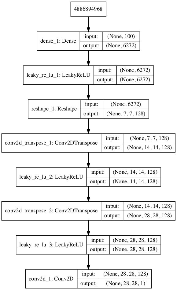
Developing a generator model requires that we transform a vector from the latent space with, 100 dimensions to a 2D array with 28×28 or 784 values.
There are a number of ways to achieve this but there is one approach that has proven effective at deep convolutional generative adversarial networks. It involves two main elements.
The first is a Dense layer as the first hidden layer that has enough nodes to represent a low-resolution version of the output image. Specifically, an image half the size (one quarter the area) of the output image would be 14×14 or 196 nodes, and an image one quarter the size (one eighth the area) would be 7×7 or 49 nodes.
We don’t just want one low-resolution version of the image; we want many parallel versions or interpretations of the input. This is a pattern in convolutional neural networks where we have many parallel filters resulting in multiple parallel activation maps, called feature maps, with different interpretations of the input. We want the same thing in reverse: many parallel versions of our output with different learned features that can be collapsed in the output layer into a final image. The model needs space to invent, create, or generate.
Therefore, the first hidden layer, the Dense, needs enough nodes for multiple low-resolution versions of our output image, such as 128.
1
2
# foundation for 7x7 image
model.add(Dense(128*7*7,input_dim=100))
The activations from these nodes can then be reshaped into something image-like to pass into a convolutional layer, such as 128 different 7×7 feature maps.
1
model.add(Reshape((7,7,128)))
The next major architectural innovation involves upsampling the low-resolution image to a higher resolution version of the image.
There are two common ways to do this upsampling process, sometimes called deconvolution.
One way is to use an UpSampling2D layer (like a reverse pooling layer) followed by a normal Conv2D layer. The other and perhaps more modern way is to combine these two operations into a single layer, called a Conv2DTranspose. We will use this latter approach for our generator.
The Conv2DTranspose layer can be configured with a stride of (2×2) that will quadruple the area of the input feature maps (double their width and height dimensions). It is also good practice to use a kernel size that is a factor of the stride (e.g. double) to avoid a checkerboard pattern that can be observed when upsampling.
This can be repeated to arrive at our 28×28 output image.
Again, we will use the LeakyReLU with a default slope of 0.2, reported as a best practice when training GAN models.
The output layer of the model is a Conv2D with one filter and a kernel size of 7×7 and ‘same’ padding, designed to create a single feature map and preserve its dimensions at 28×28 pixels. A sigmoid activation is used to ensure output values are in the desired range of [0,1].
The define_generator() function below implements this and defines the generator model.
Note: the generator model is not compiled and does not specify a loss function or optimization algorithm. This is because the generator is not trained directly. We will learn more about this in the next section.
Running the example summarizes the layers of the model and their output shape.
We can see that, as designed, the first hidden layer has 6,272 parameters or 128 * 7 * 7, the activations of which are reshaped into 128 7×7 feature maps. The feature maps are then upscaled via the two Conv2DTranspose layers to the desired output shape of 28×28, until the output layer, where a single activation map is output.
A plot of the model is also created and we can see that the model expects a 100-element point from the latent space as input and will generate an image as output.
Note: creating this plot assumes that the pydot and graphviz libraries are installed. If this is a problem, you can comment out the import statement for the plot_model function and the call to the plot_model function.
Plot of the Generator Model in the MNIST GAN
This model cannot do much at the moment.
Nevertheless, we can demonstrate how to use it to generate samples. This is a helpful demonstration to understand the generator as just another model, and some of these elements will be useful later.
The array of random numbers can then be reshaped into samples, that is n rows with 100 elements per row. The generate_latent_points() function below implements this and generates the desired number of points in the latent space that can be used as input to the generator model.
1
2
3
4
5
6
7
# generate points in latent space as input for the generator
def generate_latent_points(latent_dim,n_samples):
# generate points in the latent space
x_input=randn(latent_dim *n_samples)
# reshape into a batch of inputs for the network
x_input=x_input.reshape(n_samples,latent_dim)
returnx_input
Next, we can use the generated points as input to the generator model to generate new samples, then plot the samples.
We can update the generate_fake_samples() function from the previous section to take the generator model as an argument and use it to generate the desired number of samples by first calling the generate_latent_points() function to generate the required number of points in latent space as input to the model.
The updated generate_fake_samples() function is listed below and returns both the generated samples and the associated class labels.
1
2
3
4
5
6
7
8
9
# use the generator to generate n fake examples, with class labels
We can then plot the generated samples as we did the real MNIST examples in the first section by calling the imshow() function with the reversed grayscale color map.
The complete example of generating new MNIST images with the untrained generator model is listed below.
1
2
3
4
5
6
7
8
9
10
11
12
13
14
15
16
17
18
19
20
21
22
23
24
25
26
27
28
29
30
31
32
33
34
35
36
37
38
39
40
41
42
43
44
45
46
47
48
49
50
51
52
53
54
55
56
57
58
59
60
61
62
63
# example of defining and using the generator model
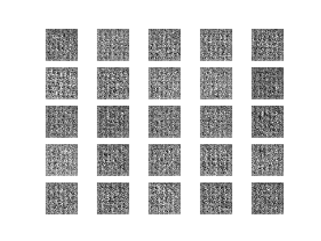
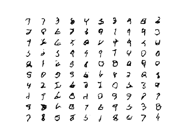
Running the example generates 25 examples of fake MNIST images and visualizes them on a single plot of 5 by 5 images.
As the model is not trained, the generated images are completely random pixel values in [0, 1].
Example of 25 MNIST Images Output by the Untrained Generator Model
Now that we know how to define and use the generator model, the next step is to train the model.
How to Train the Generator Model
The weights in the generator model are updated based on the performance of the discriminator model.
When the discriminator is good at detecting fake samples, the generator is updated more, and when the discriminator model is relatively poor or confused when detecting fake samples, the generator model is updated less.
This defines the zero-sum or adversarial relationship between these two models.
There may be many ways to implement this using the Keras API, but perhaps the simplest approach is to create a new model that combines the generator and discriminator models.
Specifically, a new GAN model can be defined that stacks the generator and discriminator such that the generator receives as input random points in the latent space and generates samples that are fed into the discriminator model directly, classified, and the output of this larger model can be used to update the model weights of the generator.
To be clear, we are not talking about a new third model, just a new logical model that uses the already-defined layers and weights from the standalone generator and discriminator models.
Only the discriminator is concerned with distinguishing between real and fake examples, therefore the discriminator model can be trained in a standalone manner on examples of each, as we did in the section on the discriminator model above.
The generator model is only concerned with the discriminator’s performance on fake examples. Therefore, we will mark all of the layers in the discriminator as not trainable when it is part of the GAN model so that they can not be updated and overtrained on fake examples.
When training the generator via this logical GAN model, there is one more important change. We want the discriminator to think that the samples output by the generator are real, not fake. Therefore, when the generator is trained as part of the GAN model, we will mark the generated samples as real (class 1).
Why would we want to do this?
We can imagine that the discriminator will then classify the generated samples as not real (class 0) or a low probability of being real (0.3 or 0.5). The backpropagation process used to update the model weights will see this as a large error and will update the model weights (i.e. only the weights in the generator) to correct for this error, in turn making the generator better at generating good fake samples.
Let’s make this concrete.
Inputs: Point in latent space, e.g. a 100 element vector of Gaussian random numbers.
Outputs: Binary classification, likelihood the sample is real (or fake).
The define_gan() function below takes as arguments the already-defined generator and discriminator models and creates the new logical third model subsuming these two models. The weights in the discriminator are marked as not trainable, which only affects the weights as seen by the GAN model and not the standalone discriminator model.
The GAN model then uses the same binary cross entropy loss function as the discriminator and the efficient Adam version of stochastic gradient descent with the learning rate of 0.0002 and momentum 0.5, recommended when training deep convolutional GANs.
1
2
3
4
5
6
7
8
9
10
11
12
13
14
# define the combined generator and discriminator model, for updating the generator
Making the discriminator not trainable is a clever trick in the Keras API.
The trainable property impacts the model after it is compiled. The discriminator model was compiled with trainable layers, therefore the model weights in those layers will be updated when the standalone model is updated via calls to the train_on_batch() function.
The discriminator model was then marked as not trainable, added to the GAN model, and compiled. In this model, the model weights of the discriminator model are not trainable and cannot be changed when the GAN model is updated via calls to the train_on_batch() function. This change in the trainable property does not impact the training of standalone discriminator model.
This behavior is described in the Keras API documentation here:
A plot of the model is also created and we can see that the model expects a 100-element point in latent space as input and will predict a single output classification label.
Note: creating this plot assumes that the pydot and graphviz libraries are installed. If this is a problem, you can comment out the import statement for the plot_model function and the call to the plot_model() function.
Plot of the Composite Generator and Discriminator Model in the MNIST GAN
Training the composite model involves generating a batch worth of points in the latent space via the generate_latent_points() function in the previous section, and class=1 labels and calling the train_on_batch() function.
The train_gan() function below demonstrates this, although is pretty simple as only the generator will be updated each epoch, leaving the discriminator with default model weights.
# prepare points in latent space as input for the generator
x_gan=generate_latent_points(latent_dim,n_batch)
# create inverted labels for the fake samples
y_gan=ones((n_batch,1))
# update the generator via the discriminator's error
gan_model.train_on_batch(x_gan,y_gan)
Instead, what is required is that we first update the discriminator model with real and fake samples, then update the generator via the composite model.
This requires combining elements from the train_discriminator() function defined in the discriminator section above and the train_gan() function defined above. It also requires that we enumerate over both epochs and batches within in an epoch.
The complete train function for updating the discriminator model and the generator (via the composite model) is listed below.
There are a few things to note in this model training function.
First, the number of batches within an epoch is defined by how many times the batch size divides into the training dataset. We have a dataset size of 60K samples, so with rounding down, there are 234 batches per epoch.
The discriminator model is updated once per batch by combining one half a batch of fake and real examples into a single batch via the vstack() NumPy function. You could update the discriminator with each half batch separately (recommended for more complex datasets) but combining the samples into a single batch will be faster over a long run, especially when training on GPU hardware.
Finally, we report the loss each batch. It is critical to keep an eye on the loss over batches. The reason for this is that a crash in the discriminator loss indicates that the generator model has started generating rubbish examples that the discriminator can easily discriminate.
Monitor the discriminator loss and expect it to hover around 0.5 to 0.8 per batch on this dataset. The generator loss is less critical and may hover between 0.5 and 2 or higher on this dataset. A clever programmer might even attempt to detect the crashing loss of the discriminator, halt, and then restart the training process.
We almost have everything we need to develop a GAN for the MNIST handwritten digits dataset.
One remaining aspect is the evaluation of the model.
How to Evaluate GAN Model Performance
Generally, there are no objective ways to evaluate the performance of a GAN model.
We cannot calculate this objective error score for generated images. It might be possible in the case of MNIST images because the images are so well constrained, but in general, it is not possible (yet).
Instead, images must be subjectively evaluated for quality by a human operator. This means that we cannot know when to stop training without looking at examples of generated images. In turn, the adversarial nature of the training process means that the generator is changing after every batch, meaning that once “good enough” images can be generated, the subjective quality of the images may then begin to vary, improve, or even degrade with subsequent updates.
There are three ways to handle this complex training situation.
Periodically evaluate the classification accuracy of the discriminator on real and fake images.
Periodically generate many images and save them to file for subjective review.
Periodically save the generator model.
All three of these actions can be performed at the same time for a given training epoch, such as every five or 10 training epochs. The result will be a saved generator model for which we have a way of subjectively assessing the quality of its output and objectively knowing how well the discriminator was fooled at the time the model was saved.
Training the GAN over many epochs, such as hundreds or thousands of epochs, will result in many snapshots of the model that can be inspected and from which specific outputs and models can be cherry-picked for later use.
First, we can define a function called summarize_performance() function that will summarize the performance of the discriminator model. It does this by retrieving a sample of real MNIST images, as well as generating the same number of fake MNIST images with the generator model, then evaluating the classification accuracy of the discriminator model on each sample and reporting these scores.
1
2
3
4
5
6
7
8
9
10
11
12
# evaluate the discriminator, plot generated images, save generator model
Next, we can update the summarize_performance() function to both save the model and to create and save a plot generated examples.
The generator model can be saved by calling the save() function on the generator model and providing a unique filename based on the training epoch number.
1
2
3
4
...
# save the generator model tile file
filename='generator_model_%03d.h5'%(epoch+1)
g_model.save(filename)
We can develop a function to create a plot of the generated samples.
As we are evaluating the discriminator on 100 generated MNIST images, we can plot all 100 images as a 10 by 10 grid. The save_plot() function below implements this, again saving the resulting plot with a unique filename based on the epoch number.
1
2
3
4
5
6
7
8
9
10
11
12
13
14
# create and save a plot of generated images (reversed grayscale)
def save_plot(examples,epoch,n=10):
# plot images
foriinrange(n *n):
# define subplot
pyplot.subplot(n,n,1+i)
# turn off axis
pyplot.axis('off')
# plot raw pixel data
pyplot.imshow(examples[i,:,:,0],cmap='gray_r')
# save plot to file
filename='generated_plot_e%03d.png'%(epoch+1)
pyplot.savefig(filename)
pyplot.close()
The updated summarize_performance() function with these additions is listed below.
1
2
3
4
5
6
7
8
9
10
11
12
13
14
15
16
17
# evaluate the discriminator, plot generated images, save generator model
We now have everything we need to train and evaluate a GAN on the MNIST handwritten digit dataset.
The complete example is listed below.
Note: this example can run on a CPU but may take a number of hours. The example can run on a GPU, such as the Amazon EC2 p3 instances, and will complete in a few minutes.
For help on setting up an AWS EC2 instance to run this code, see the tutorial:
The chosen configuration results in the stable training of both the generative and discriminative model.
The model performance is reported every batch, including the loss of both the discriminative (d) and generative (g) models.
Note: Your results may vary given the stochastic nature of the algorithm or evaluation procedure, or differences in numerical precision. Consider running the example a few times and compare the average outcome.
In this case, the loss remains stable over the course of training.
1
2
3
4
5
6
7
8
9
10
11
12
>1, 1/234, d=0.711, g=0.678
>1, 2/234, d=0.703, g=0.698
>1, 3/234, d=0.694, g=0.717
>1, 4/234, d=0.684, g=0.740
>1, 5/234, d=0.679, g=0.757
>1, 6/234, d=0.668, g=0.777
...
>100, 230/234, d=0.690, g=0.710
>100, 231/234, d=0.692, g=0.705
>100, 232/234, d=0.698, g=0.701
>100, 233/234, d=0.697, g=0.688
>100, 234/234, d=0.693, g=0.698
The generator is evaluated every 20 epochs, resulting in 10 evaluations, 10 plots of generated images, and 10 saved models.
In this case, we can see that the accuracy fluctuates over training. When viewing the discriminator model’s accuracy score in concert with generated images, we can see that the accuracy on fake examples does not correlate well with the subjective quality of images, but the accuracy for real examples may.
It is crude and possibly unreliable metric of GAN performance, along with loss.
1
2
3
4
5
6
7
8
9
10
>Accuracy real: 51%, fake: 78%
>Accuracy real: 30%, fake: 95%
>Accuracy real: 75%, fake: 59%
>Accuracy real: 98%, fake: 11%
>Accuracy real: 27%, fake: 92%
>Accuracy real: 21%, fake: 92%
>Accuracy real: 29%, fake: 96%
>Accuracy real: 4%, fake: 99%
>Accuracy real: 18%, fake: 97%
>Accuracy real: 28%, fake: 89%
More training, beyond some point, does not mean better quality generated images.
In this case, the results after 10 epochs are low quality, although we can see that the generator has learned to generate centered figures in white on a back background (recall we have inverted the grayscale in the plot).
Plot of 100 GAN Generated MNIST Figures After 10 Epochs
After 20 or 30 more epochs, the model begins to generate very plausible MNIST figures, suggesting that 100 epochs are probably not required for the chosen model configurations.
Plot of 100 GAN Generated MNIST Figures After 40 Epochs
The generated images after 100 epochs are not greatly different, but I believe I can detect less blocky-ness in the curves.
Plot of 100 GAN Generated MNIST Figures After 100 Epochs
How to Use the Final Generator Model to Generate Images
Once a final generator model is selected, it can be used in a standalone manner for your application.
This involves first loading the model from file, then using it to generate images. The generation of each image requires a point in the latent space as input.
The complete example of loading the saved model and generating images is listed below. In this case, we will use the model saved after 100 training epochs, but the model saved after 40 or 50 epochs would work just as well.
1
2
3
4
5
6
7
8
9
10
11
12
13
14
15
16
17
18
19
20
21
22
23
24
25
26
27
28
29
30
31
32
33
# example of loading the generator model and generating images
from keras.models import load_model
from numpy.random import randn
from matplotlib import pyplot
# generate points in latent space as input for the generator
def generate_latent_points(latent_dim,n_samples):
# generate points in the latent space
x_input=randn(latent_dim *n_samples)
# reshape into a batch of inputs for the network
x_input=x_input.reshape(n_samples,latent_dim)
returnx_input
# create and save a plot of generated images (reversed grayscale)
def save_plot(examples,n):
# plot images
foriinrange(n *n):
# define subplot
pyplot.subplot(n,n,1+i)
# turn off axis
pyplot.axis('off')
# plot raw pixel data
pyplot.imshow(examples[i,:,:,0],cmap='gray_r')
pyplot.show()
# load model
model=load_model('generator_model_100.h5')
# generate images
latent_points=generate_latent_points(100,25)
# generate images
X=model.predict(latent_points)
# plot the result
save_plot(X,5)
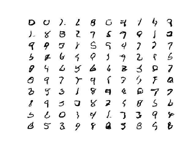
Running the example first loads the model, samples 25 random points in the latent space, generates 25 images, then plots the results as a single image.
We can see that most of the images are plausible, or plausible pieces of handwritten digits.
Example of 25 GAN Generated MNIST Handwritten Images
The latent space now defines a compressed representation of MNIST handwritten digits.
You can experiment with generating different points in this space and see what types of numbers they generate.
The example below generates a single handwritten digit using a vector of all 0.0 values.
1
2
3
4
5
6
7
8
9
10
11
12
13
# example of generating an image for a specific point in the latent space
from keras.models import load_model
from numpy import asarray
from matplotlib import pyplot
# load model
model=load_model('generator_model_100.h5')
# all 0s
vector=asarray([[0.0for_inrange(100)]])
# generate image
X=model.predict(vector)
# plot the result
pyplot.imshow(X[0,:,:,0],cmap='gray_r')
pyplot.show()
Note: Your results may vary given the stochastic nature of the algorithm or evaluation procedure, or differences in numerical precision. Consider running the example a few times and compare the average outcome.
In this case, a vector of all zeros results in a handwritten 9 or maybe an 8. You can then try navigating the space and see if you can generate a range of similar, but different handwritten digits.
Example of a GAN Generated MNIST Handwritten Digit for a Vector of Zeros
Extensions
This section lists some ideas for extending the tutorial that you may wish to explore.
TanH Activation and Scaling. Update the example to use the tanh activation function in the generator and scale all pixel values to the range [-1, 1].
Change Latent Space. Update the example to use a larger or smaller latent space and compare the quality of the results and speed of training.
Batch Normalization. Update the discriminator and/or the generator to make use of batch normalization, recommended for DCGAN models.
Label Smoothing. Update the example to use one-sided label smoothing when training the discriminator, specifically change the target label of real examples from 1.0 to 0.9, and review the effects on image quality and speed of training.
Model Configuration. Update the model configuration to use deeper or more shallow discriminator and/or generator models, perhaps experiment with the UpSampling2D layers in the generator.
If you explore any of these extensions, I’d love to know.
Post your findings in the comments below.
Further Reading
This section provides more resources on the topic if you are looking to go deeper.
Books
Chapter 20. Deep Generative Models, Deep Learning, 2016.
# foundation for 7×7 image
model.add(Dense(128 * 7 * 7, input_dim=100)).
I sometimes see input_dim = 100, so when do we need the comma?
My second question. The output of the generator must match the input of the discriminator in our gan right? so what’s about these (7,7) filter size?
Thanks a lot for elaborate on this
best regards
You need the command when specifying “shape” instead of “dim”.
Correct, input of D matches output of G. 7×7 is our starting point for the random image that we scale up to the desired size with the appropriate layers.
Thanks Jason.
The input of the discriminator is a 28,28 image with 1colorchannel. If we provide a different shape we probably get an error.
Our output is conv2dtransposed to match this size 28,28 but what about these 7×7 filters? In the GAN we stack the output of the generator as input in the discriminator so I would assume we need (batch_size, 28,28,1) which is different from the return value from the generator with this 7×7 filters. Maybe I am missing something here.
Again thanks so much for this blog. Your speed and exlanations are invaluable!
Thank you for the comprehensive notes Jason. I’ve done some work with deep CNNs as regular classifiers but these examples are a first toe in the water in the world of GANs. Your explanations are very clear.
This worked well. There were problems with the discriminator collapsing to zero on occasions. This seems to be a known feature of GANs. Do any established GAN hacks help with this?
Looking at the discriminator after 100 epochs, it was in a confused state where everything passed into it was circa 50% probability real/fake. I colour coded some generated examples based on disriminator probability (red = fake, green = real, blue = unsure based on an arbitrary banding) and as you mentioned the subjective versus discriminator output does not always tie up. (example posted on linkedin). There was not enough spread in discriminator probability output to make this meaningful.
Finding a mechanism to measure how good the generator is in order to save the ‘best’ model would be good, otherwise it would seem to remain very subjective as to what the best generator is.
I got mine trained and completed in 28 hours using CPU mode, i7, 8th gen PC. The digit images it generated looked good with 90% recognizable. It’s very good tutorial. Thanks.
Thanks for the great tutorial, I am trying to make a GAN for an Ising model, Where I would like to pass an extra argument of temperature to the Generator along with the noise. Is it possible to do in a Transpose CNN network used as a generator?
I tried some of your suggestions :
– I tried tanh instead of sigmoid but quickly the discriminator loss was less than 0.5 (around 0.2)
– I added batchNormalization into the generator but I did not see a big differences in the results
model = Sequential()
# foundation for 7×7 image
n_nodes = 128 * 7 * 7
model.add(Dense(n_nodes, input_dim=latent_dim))
model.add(LeakyReLU(alpha=0.2))
model.add(BatchNormalization(momentum=0.8))
model.add(Reshape((7, 7, 128)))
# upsample to 14×14
model.add(Conv2DTranspose(128, (4,4), strides=(2,2), padding=’same’))
model.add(LeakyReLU(alpha=0.2))
model.add(BatchNormalization(momentum=0.8))
# upsample to 28×28
model.add(Conv2DTranspose(128, (4,4), strides=(2,2), padding=’same’))
model.add(LeakyReLU(alpha=0.2))
model.add(BatchNormalization(momentum=0.8))
model.add(Conv2D(1, (7,7), activation=’sigmoid’, padding=’same’))
return model
– I changed the latent_dim parameter from 100 to 5000. The computed model was bigger each time, the computed time was longer each time, from 45 mn for 100 to 120 mn for 5000 on an GPU Nvidia k100 and the results were better each time.
I am keep working on it
Hey Jason
I never understood how dropout works in case of conv layers. Theoretically it looks a bit weird to me. https://towardsdatascience.com/dropout-on-convolutional-layers-is-weird-5c6ab14f19b2
This article supports my intuitions.
I tried your model without the dropout and it achieved an accuracy of real:100% fake :3% after the 80th epoch.
If my understanding is correct, this means our generator has become very competent in fooling the discriminator.
How do you view these results? And what is your view on dropouts applied on conv layers?
Hi, Jason, thants for the great post again, from your advise, I used tanh function on the generator, changed dataset ranges to [-1, 1], but I’ve got black images from the generator, so I changed the generator’s last layer’s filter size to smaller values, to (3, 3), I don’t know why, but it worked.
Why discriminator are updated twiced by train_on_batch ? I think, this step will update twice the paramters. Is it so? But in pytorch, we just accumulated all the gradients (for the real data and generated data) then update paramters by a single step.
Thanks for your great post! I have learn a lot from it.But when I train the model,I got the following warning:
/opt/conda/lib/python3.6/site-packages/keras/engine/training.py:297: UserWarning: Discrepancy between trainable weights and collected trainable weights, did you set model.trainable without calling model.compile after ?
‘Discrepancy between trainable weights and collected trainable’
Thanks for your reply!
And I want to know how to get the state-of-art performance? Even I have tried every hack you list,I find the some generate images are great,while others still can’t recognize what number it is? Are there some suggestions?
Hi Jason,
Thanks for sharing this tutorial with us. It is very helpful and well written.
I just wanted to ask a question. If I have a dataset of over a million images in color and each image is 28 x 28 pixels, which GAN architecture would you recommend me please?
Thanks in advance.
I got a question. If the generator and discriminator and now combined, what’s the point of keeping the “original” discriminator (besides for evaluating its loss value)?
I understand that the discriminator (the one that’s not combined) is updated as a standalone model. But what when you mean that “the generator must be updated via the discriminator.”,
are you referring to the “original” discriminator? Or the one from the combined model? If the latest, how it is that the generator is using it to update itself, it the “combined” discriminator’s weights are non-trainable? I feel there’s a crucial step I’m missing.
I have a question about the train function which takes the d_model, g_model and gan_model (and others) as input.
In that function, there is a d_model and g_model. There is also a d_model in gan_model and g_model in gan_model.
You run d_model.train_on_batch to update the d_model weights. After that the updated weights need to be passed to the d_model in gan_model before you can run gan_model.train_on_batch, but I don’t see any line of code doing that.
Similarly, after you train the gan_model to update the g_model in gan_model weights, those weights should be passed to the g_model for the next fake image generation. Again, I don’t see any code that serves that purpose.
Do these all have to do with the models are somehow saved in a global manner? Would you please please explain it?
Nice Explainaition.
i have one question.
I want to calculate accuracy that wether the final image generated are not much diff from original ones given as input.
In that i will require the digits that are inside the images in matrix from.
Is there any way that i can get the digits from inside images using any model, so that i can compare the original ones and final ones?
Please reply!
Thankyou in advance!
I would like to develop a generative model that can take two images as input ( They are two different images but relevant to each other ), learn the relation between the images and generative two images as output maintaining consistency between the two images. Could you please suggest how to approach this problem?
But, don’t we need to shuffle the real and fake samples when training the discriminator model, because we have just stacked the real and fake samples on each other.
So, don’t you think we should shuffle because I have heard people saying that your data should always be shuffled so that your model trains better.
I had an issue, I was getting weird generated images, so I copied your whole code and pasted it in google colab, and then ran it, and I still got weird generated images.
But by these Models, it couldn’t generate good images in even 200 epochs. (We could see that it is trying to generate some images, but they were not good, as you achieved in 100 epochs).
Then I changed the discriminator model a little, and changed it to this:
And left the generator model the same as the one that I mentioned before in this comment.
I just removed the batch Normalization and Leaky relu layer in the discriminator starting stages, and just replaced the leaky relu activation with softmax activation (which, for me, doesn’t make any sense. Because I have used softmax only in the last layers of models to make predictions, And I never thought of using softmax in a GAN, in the discriminator starting layers).
But then, to my surprise, the generated images got good in almost 90 epochs, outperforming the previous model. I thought that maybe this was just some kind of luck, So, I ran these 2 discriminator model, 2 to 4 times, and each time, the discriminator model with softmax was a lot better than the other.
Hello Jason, I figured out what happened. Both the models (one with softmax activation in the first layer of discriminator and the one that I mentioned in the starting of the comment, which had batch Normalization and Max Pooling in it ), were performing the same. I tested the both the models on pycharm (python IDE), and they both generated image with the same precision. I think, this was some fault with Google Colab. Sorry for the trouble.
But Now, Since they both generated images with the same precision, I wanted to ask that shouldn’t the images generated by the model, which had softmax activation in it, be very bad. Because, putting softmax in the first layer of discriminator makes no sense to me. So, why were they good?
Things have work great when I train the model continuously. But when I save the Gen and Disc models as h5 files and try to further train after loading the saved files, the discriminator always fails to keep up and the loss grows over time. I even tried changing the learning rates of the two optimizers so that the Disc learns faster but this only slowed things down. Any recommendations?
I’m training my model in Google Colab and it times-out after some time. So I tried to continue where I left off. I realize now that the model is experiencing mode collapse. I can see that the output images are all looking the same now. Any recommendations on how to address it?
I realized what is happening. The discriminator was set to trainable=False by default when the model was being loaded. Setting that parameter to true has resolved the problem. Thanks for taking the time to respond to me.
Dear Jason,
Thanks for compiling very good starter on DCGAN. I appreciate if you increase the reading area to width of a screen and font size little bigger
Thanks a lot for the tutorial.
A great example that encapsulates everything.
I ran this on google collab using a GPU and it runs quite fast.
One question though, if the discriminator accuracy on fake data is ~90% doesn’t it mean the generator is doing a bad job? I also don’t understand why would the accuracy on the real data be that low. it looks like the disc can identify fake data easily but can’t identify real data, wouldn’t that mean its just a really bad disc + really bad gen?
Could you also train one GAN for each class of data, thereby resulting in an output of images that can be labelled trivially corresponding to that class?
Hey Guys, Thanks for the tutorial. Is any of you have a save of the generator model at any epochs ? I launched it this night and my google collab session stopped… I lost saves from epochs 10 and 20. If any of you can give me a save from the generator model so i don’t have to restart the whole thing, it would be great.
i had applied your code on my handritten character dataset, but it is giving 100% accuracy foreal and fake examples like this after 100 epochs
>100, 81/92, d=0.000, g=9.672
>100, 82/92, d=0.000, g=9.683
>100, 83/92, d=0.000, g=9.765
>100, 84/92, d=0.000, g=9.668
>100, 85/92, d=0.000, g=9.816
>100, 86/92, d=0.000, g=9.730
>100, 87/92, d=0.000, g=9.758
>100, 88/92, d=0.000, g=9.740
>100, 89/92, d=0.000, g=9.716
>100, 90/92, d=0.000, g=9.735
>100, 91/92, d=0.000, g=9.804
>100, 92/92, d=0.000, g=9.763
>Accuracy real: 100%, fake: 100%
i m not getting it and it is giving blank space during generation of images when i had evaluated the model. kindly reply
Thank you for your tutorial. It is very helpful for a beginner to understand the concepts of GAN. Sir, can we use GAN for regression type problems for generating more samples in the cases of small datasets? Could you please share some links for that?
Thanks for your awesome tutorials. I often find them a great reference when implementing my own models.
I have a question… In the generator you use a normal distribution, which is standard practice in GANs. But instead of using the generator to produce a sample for training the discriminator, you instead use a uniform distribution to mimic the original normalised data.
I wanted to know if this was normal practice, because from my understanding I thought you would pull a distribution straight from the Generator along with real samples to train the discriminator. The only reason I can think of is drawing a uniform distribution bypasses the need to do a forward pass through the generator, saving on computations. However, doesn’t the discriminator want to be exposed to improved fake data as the generator performance improves?
I hope this makes sense… basically why do you use a uniform distribution instead of drawing fake data from the Generator when training the discriminator?
Thanks so much for the nice tutorial. I have 2 questions:
1) Ideally, we should have an accuracy for “real” and “fake” as close to 1, while having a loss for both the generative & discriminative, as close to 0? Is my understanding correct? Now talking about “reality”, what is the usual trade-off between those values?
2) I have used your tutorial for some revision of DL techniques, for binary classification, but using spreadsheets instead of images. After some tuning of your code, I managed to put my projecto to work. However, I am getting values like this:
Unfortunately, I haven’t had much experience with GANs, other than your original project, and the one of my own. Would you say those values are “acceptable” to start predicting samples from the minority-class?
Indeed, accuracy is a poor metric, which raises 2 additional questions:
1) Why was accuracy chose here then? I think it was just as some kind of “glimpse to the behaviour of the Generative VS the Discriminative networks”, wasn’t it?
2) I have read the paper “Pros and Cons of GAN Evaluation Measures” suggested in your article “How to Evaluate Generative Adversarial Networks”. I cannot go with qualitative evaluation since, like I said before, I am not dealing with images, but with numeric vectors and I cannot judge if they’re OK or not; on top of that, that paper basically concludes that “there isn’t a good-for-all-cases metric so far”. What I am doing right now is intuitively pick the models with highest precision – recall – F1 on toy datasets (it is the method # 24 on the aforementioned paper, which was achieved by modification of your code, replacing accuracy for those measures), pick the model that shown best metrics, and then plug those samples on another classifier network, to see how the generated samples performance go. Would it be correct?
Included accuracy out of interest, the best “metric” is to generate images and review them.
If you are working with MNIST directly, then a classification of generated images sounds reasonable, at least if you use a pre-trained model on all of MNIST instead of the discriminator.
Thanks for great tutorial. I have confuse about the last Conv2D layer you used in the generator model. You said that: “The output layer of the model is a Conv2D with one filter and a kernel size of 7×7 and ‘same’ padding, designed to create a single feature map and preserve its dimensions at 28×28 pixels. ”
Why you chose big kernel size 7×7. We usually use smaller kernel size 3×3 or 5×5. Could you please explain it?
Hey I used your code to train the model but i dont know where it is stroing the model. when i recall the model it says that no model found ? Can you tell me what i am doing wrong
Thank you Jason. Your tutorial worked fine for me. I so much enjoy reading from you. Thank you once again.
I am currently working on deep learning steganography model, where I intend to hide colored image in another colored image (Known as the cover image).
Please how do I perform the encoding model using cycleGAN and DCGAN?
Also, how do I perform the decoding model to retrieve both the original Cover image and the secret image using CNN?
Thank you Jason. Your tutorial is so helpful. I so much enjoy reading from you.
I got a problem when I use KL loss rather than “binary__crossentropy”. Afther few epochs the discriminator has 100% accuracy over the real examples, but 0% accuracy over the fake examples.
You may be working on a regression problem and achieve zero prediction errors.
Alternately, you may be working on a classification problem and achieve 100% accuracy.
This is unusual and there are many possible reasons for this, including:
You are evaluating model performance on the training set by accident.
Your hold out dataset (train or validation) is too small or unrepresentative.
You have introduced a bug into your code and it is doing something different from what you expect.
Your prediction problem is easy or trivial and may not require machine learning.
The most common reason is that your hold out dataset is too small or not representative of the broader problem.
This can be addressed by:
Using k-fold cross-validation to estimate model performance instead of a train/test split.
Gather more data.
Use a different split of data for train and test, such as 50/50.
Hi, I was having problems using a model from a good data science book, so I copied your model and let it run for over 20 epochs. I seem to have the same problem with your model too.
The images generated are all very similar, and don’t resemble digits at all. They don’t look like completely random noise, as it is concentrated in the centre. I don’t have the same convergence that you have in your images (nor the same as in the book I used). I believe this may be ‘mode collapse’. Is it common for identical code to work differently to this extent? I’m at a loss as to what to do.
Hi James…Have you tried your code in Google Colab to compare it with a local installation of Anaconda? You could be dealing with some library differences.
As an update… the issue seems to be with Apple’s metal plugin for tensorflow on M1 Macs. It seems that when performing certain computations on the GPU, problems occur. It’s been posted on the Apple developer forum, but 6 months later still hasn’t been solved. So if you have an M1 Mac, perhaps use the standard tensorflow (not Apple’s version).
I ran the code again on Colab and on my own machine (without Apple’s tensorflow plugin), and had no issues.
I have doubt regarding the data. I have data from accelerometer and want to augment data for the same. I have aShort time fourier transform of this accelerometer data. This fourier transform show if a person has fallen from the bed or not. So I want to augment data for such case where person falls from the bed. Can I use GAN or VAE for such applciation. I tired to implement it, but I was not successful. Can you guide me throug this please?


 From Scratch with Keras")


 From Scratch")
 in Keras")
Hi Jason.
Great tutorial.when is your book on GAN coming out?will you be doing a tutorial on transfer learning in relation to GAN?
Thanks!
I hope to have the book ready in a few weeks.
Great suggestion!
hello Mr. Jason,
pyplot.imshow(trainX[i], cmap=’gray’) and pyplot.imshow(testX[i], cmap=’gray’) are showing error as you have passed variable ‘i’.
thanks for the fantastic tutorials.
I am not getting an error. What error are you getting exactly?
I have some suggestions here:
https://machinelearningmastery.com/faq/single-faq/why-does-the-code-in-the-tutorial-not-work-for-me
Great thanks.
2 Questions if I may.
# foundation for 7×7 image
model.add(Dense(128 * 7 * 7, input_dim=100)).
I sometimes see input_dim = 100, so when do we need the comma?
My second question. The output of the generator must match the input of the discriminator in our gan right? so what’s about these (7,7) filter size?
Thanks a lot for elaborate on this
best regards
Great questions!
You need the command when specifying “shape” instead of “dim”.
Correct, input of D matches output of G. 7×7 is our starting point for the random image that we scale up to the desired size with the appropriate layers.
Does that help?
Thanks Jason.
The input of the discriminator is a 28,28 image with 1colorchannel. If we provide a different shape we probably get an error.
Our output is conv2dtransposed to match this size 28,28 but what about these 7×7 filters? In the GAN we stack the output of the generator as input in the discriminator so I would assume we need (batch_size, 28,28,1) which is different from the return value from the generator with this 7×7 filters. Maybe I am missing something here.
Again thanks so much for this blog. Your speed and exlanations are invaluable!
The output of the generator is a 28x28x1 matrix.
Thank you for the comprehensive notes Jason. I’ve done some work with deep CNNs as regular classifiers but these examples are a first toe in the water in the world of GANs. Your explanations are very clear.
This worked well. There were problems with the discriminator collapsing to zero on occasions. This seems to be a known feature of GANs. Do any established GAN hacks help with this?
Looking at the discriminator after 100 epochs, it was in a confused state where everything passed into it was circa 50% probability real/fake. I colour coded some generated examples based on disriminator probability (red = fake, green = real, blue = unsure based on an arbitrary banding) and as you mentioned the subjective versus discriminator output does not always tie up. (example posted on linkedin). There was not enough spread in discriminator probability output to make this meaningful.
Finding a mechanism to measure how good the generator is in order to save the ‘best’ model would be good, otherwise it would seem to remain very subjective as to what the best generator is.
Yes, the hacks will help with reducing the likelihood of a collapse.
I will cover good metrics/loss in the future. WGAN might be the best here. I have 2 posts on the topic coming.
Thanks, I’ll look out for it. In the meantime will use this example as a sand pit for trying some of the suggested hacks. Cheers
Great idea!
I got mine trained and completed in 28 hours using CPU mode, i7, 8th gen PC. The digit images it generated looked good with 90% recognizable. It’s very good tutorial. Thanks.
Well done Phillip!
RESPECT
Hi Jason,
Thanks for the great tutorial, I am trying to make a GAN for an Ising model, Where I would like to pass an extra argument of temperature to the Generator along with the noise. Is it possible to do in a Transpose CNN network used as a generator?
Sure, perhaps look at some of the conditional GANs, for example:
https://machinelearningmastery.com/how-to-develop-a-conditional-generative-adversarial-network-from-scratch/
Do you have a github link of above complete code?
The complete code is listed in the above tutorial, you can copy and paste it directly.
If you need help, see this:
https://machinelearningmastery.com/faq/single-faq/how-do-i-copy-code-from-a-tutorial
Hello Jason
I tried some of your suggestions :
– I tried tanh instead of sigmoid but quickly the discriminator loss was less than 0.5 (around 0.2)
– I added batchNormalization into the generator but I did not see a big differences in the results
model = Sequential()
# foundation for 7×7 image
n_nodes = 128 * 7 * 7
model.add(Dense(n_nodes, input_dim=latent_dim))
model.add(LeakyReLU(alpha=0.2))
model.add(BatchNormalization(momentum=0.8))
model.add(Reshape((7, 7, 128)))
# upsample to 14×14
model.add(Conv2DTranspose(128, (4,4), strides=(2,2), padding=’same’))
model.add(LeakyReLU(alpha=0.2))
model.add(BatchNormalization(momentum=0.8))
# upsample to 28×28
model.add(Conv2DTranspose(128, (4,4), strides=(2,2), padding=’same’))
model.add(LeakyReLU(alpha=0.2))
model.add(BatchNormalization(momentum=0.8))
model.add(Conv2D(1, (7,7), activation=’sigmoid’, padding=’same’))
return model
– I changed the latent_dim parameter from 100 to 5000. The computed model was bigger each time, the computed time was longer each time, from 45 mn for 100 to 120 mn for 5000 on an GPU Nvidia k100 and the results were better each time.
I am keep working on it
Keep latent small, at 100.
Perhaps test MSE loss function. It works great!
Hey Jason
I never understood how dropout works in case of conv layers. Theoretically it looks a bit weird to me.
https://towardsdatascience.com/dropout-on-convolutional-layers-is-weird-5c6ab14f19b2
This article supports my intuitions.
I tried your model without the dropout and it achieved an accuracy of real:100% fake :3% after the 80th epoch.
If my understanding is correct, this means our generator has become very competent in fooling the discriminator.
How do you view these results? And what is your view on dropouts applied on conv layers?
With a GAN, you want both the D and the G to have the same skill. If one does a lot better than the other, you will get a failure mode:
https://machinelearningmastery.com/practical-guide-to-gan-failure-modes/
Hi, Jason, thants for the great post again, from your advise, I used tanh function on the generator, changed dataset ranges to [-1, 1], but I’ve got black images from the generator, so I changed the generator’s last layer’s filter size to smaller values, to (3, 3), I don’t know why, but it worked.
Nice work!
Hi Jason
Thanks for the tutorial
Why you didn’t augment the channels of the fake images to 3 as you did for the real images?
Fake image are generated with 3 dimensions directly.
Hi Sir,
Do you have any related paper on this project?
please do reply.
Yes, I have a book on the topic:
https://machinelearningmastery.com/generative_adversarial_networks/
Also, there are papers listed in this post in the “further reading” section.
Why discriminator are updated twiced by train_on_batch ? I think, this step will update twice the paramters. Is it so? But in pytorch, we just accumulated all the gradients (for the real data and generated data) then update paramters by a single step.
There are many ways to implement GANs.
Hai Jason, how can i change MNIST dataset in the above code to offline dataset. Please share some reference to do so.
You can load your dataset as a numpy array:
https://machinelearningmastery.com/how-to-load-and-manipulate-images-for-deep-learning-in-python-with-pil-pillow/
Thanks Jason. but i have a large dataset and i am following the steps given by you in the below link.
https://machinelearningmastery.com/how-to-load-large-datasets-from-directories-for-deep-learning-with-keras/
I want to apply my dataset in semi supervised GAN as in
https://machinelearningmastery.com/semi-supervised-generative-adversarial-network/.
DId you cover these kind of information in any of your Ebooks??? if so, please share the link
You might need to use a custom data loader as the GANs are probably not compatible with the image data generator.
I mostly load all data into RAM when fitting GANs. E.g. use an EC2 instance with 64+ GB of RAM.
Thanks for your great post! I have learn a lot from it.But when I train the model,I got the following warning:
/opt/conda/lib/python3.6/site-packages/keras/engine/training.py:297: UserWarning: Discrepancy between trainable weights and collected trainable weights, did you set
model.trainablewithout callingmodel.compileafter ?‘Discrepancy between trainable weights and collected trainable’
does it matter?
You can safely ignore this warning.
Thanks for your reply!
And I want to know how to get the state-of-art performance? Even I have tried every hack you list,I find the some generate images are great,while others still can’t recognize what number it is? Are there some suggestions?
Best best advice is to test different models, different configurations, etc.
Hi Jason,
Thanks for sharing this tutorial with us. It is very helpful and well written.
I just wanted to ask a question. If I have a dataset of over a million images in color and each image is 28 x 28 pixels, which GAN architecture would you recommend me please?
Thanks in advance.
You’re welcome.
Perhaps start with a simple DCGAN and a smaller sample of your data and tune the model to discover what works well/best.
Start with some of the tutorials here to get ideas of model architectures and tuning tricks:
https://machinelearningmastery.com/start-here/#gans
Hi Jason,
Excellent tutorial.
I got a question. If the generator and discriminator and now combined, what’s the point of keeping the “original” discriminator (besides for evaluating its loss value)?
Thanks.
The discriminator must be updated as a standalone model.
The generator must be updated via the discriminator.
In the end the discriminator and combined model are discarded and we keep the standalone generator.
For more on GAN basics, start here:
https://machinelearningmastery.com/start-here/#gans
Hi Jason, thanks for the response.
I understand that the discriminator (the one that’s not combined) is updated as a standalone model. But what when you mean that “the generator must be updated via the discriminator.”,
are you referring to the “original” discriminator? Or the one from the combined model? If the latest, how it is that the generator is using it to update itself, it the “combined” discriminator’s weights are non-trainable? I feel there’s a crucial step I’m missing.
Thanks.
See this tutorial to understand the GAN training algorithm, e.g. generator via discriminator:
https://machinelearningmastery.com/how-to-code-the-generative-adversarial-network-training-algorithm-and-loss-functions/
Excellent tutorial!
I have a question about the train function which takes the d_model, g_model and gan_model (and others) as input.
In that function, there is a d_model and g_model. There is also a d_model in gan_model and g_model in gan_model.
You run d_model.train_on_batch to update the d_model weights. After that the updated weights need to be passed to the d_model in gan_model before you can run gan_model.train_on_batch, but I don’t see any line of code doing that.
Similarly, after you train the gan_model to update the g_model in gan_model weights, those weights should be passed to the g_model for the next fake image generation. Again, I don’t see any code that serves that purpose.
Do these all have to do with the models are somehow saved in a global manner? Would you please please explain it?
The weights in g and d are shared in the combined model. Same weights, different logical models.
You can learn more here:
https://machinelearningmastery.com/how-to-code-the-generative-adversarial-network-training-algorithm-and-loss-functions/
Nice Explainaition.
i have one question.
I want to calculate accuracy that wether the final image generated are not much diff from original ones given as input.
In that i will require the digits that are inside the images in matrix from.
Is there any way that i can get the digits from inside images using any model, so that i can compare the original ones and final ones?
Please reply!
Thankyou in advance!
Thanks.
You could use a model trained on mnist to classify the generated images.
I would like to develop a generative model that can take two images as input ( They are two different images but relevant to each other ), learn the relation between the images and generative two images as output maintaining consistency between the two images. Could you please suggest how to approach this problem?
I’m not aware of an architecture that can do this, perhaps start with a cyclegan or pix2pix and explore prototypes.
Jason,
respect for outstanding work!
Thanks!
Hello sir, it was a really a great tutorial.
But, don’t we need to shuffle the real and fake samples when training the discriminator model, because we have just stacked the real and fake samples on each other.
So, don’t you think we should shuffle because I have heard people saying that your data should always be shuffled so that your model trains better.
So, why didn’t you shuffled?
We are selecting random examples each batch which has the same effect.
Hello sir, Once again, excellent tutorial !
I had an issue, I was getting weird generated images, so I copied your whole code and pasted it in google colab, and then ran it, and I still got weird generated images.
Can you please say why this is happening?
I have not used google colab:
https://machinelearningmastery.com/faq/single-faq/do-code-examples-run-on-google-colab
Hello Jason,
I know I am asking too many questions, sorry for that.
I tried the exact same code as yours only difference I changed the discriminator and generator model.
This was mine discriminator Model:
Model = Sequential([
Conv2D(32, (3, 3), padding=’same’, input_shape=in_shape),
BatchNormalization(),
LeakyReLU(alpha=0.2),
MaxPooling2D(pool_size=(2,2)),
Dropout(0.2),
Conv2D(64, (3,3), padding=’same’),
BatchNormalization(),
LeakyReLU(alpha=0.2),
MaxPooling2D(pool_size=(2,2)),
Dropout(0.3),
Conv2D(128, (3,3), padding=’same’),
BatchNormalization(),
LeakyReLU(alpha=0.2),
MaxPooling2D(pool_size=(2,2)),
Dropout(0.3),
Flatten(),
Dense(1, activation=’sigmoid’)
])
And this was the generator Model:
Model = Sequential([
Dense(128*7*7, input_dim=in_shape),
BatchNormalization(),
LeakyReLU(alpha=0.2),
Reshape((7, 7, 128)),
Conv2DTranspose(16, (3,3), strides=(2,2), padding=’same’),
BatchNormalization(),
LeakyReLU(alpha=0.2),
Conv2DTranspose(1, (4,4), strides=(2,2), activation=’sigmoid’, padding=’same’),
])
But by these Models, it couldn’t generate good images in even 200 epochs. (We could see that it is trying to generate some images, but they were not good, as you achieved in 100 epochs).
Then I changed the discriminator model a little, and changed it to this:
Model = Sequential([
Conv2D(32, (3, 3), padding=’same’, activation=’softmax’, input_shape=in_shape),
MaxPooling2D(pool_size=(2,2)),
Dropout(0.2),
Conv2D(64, (3,3), padding=’same’),
BatchNormalization(),
LeakyReLU(alpha=0.2),
MaxPooling2D(pool_size=(2,2)),
Dropout(0.3),
Conv2D(128, (3,3), padding=’same’),
BatchNormalization(),
LeakyReLU(alpha=0.2),
MaxPooling2D(pool_size=(2,2)),
Dropout(0.3),
Flatten(),
Dense(1, activation=’sigmoid’)
])
And left the generator model the same as the one that I mentioned before in this comment.
I just removed the batch Normalization and Leaky relu layer in the discriminator starting stages, and just replaced the leaky relu activation with softmax activation (which, for me, doesn’t make any sense. Because I have used softmax only in the last layers of models to make predictions, And I never thought of using softmax in a GAN, in the discriminator starting layers).
But then, to my surprise, the generated images got good in almost 90 epochs, outperforming the previous model. I thought that maybe this was just some kind of luck, So, I ran these 2 discriminator model, 2 to 4 times, and each time, the discriminator model with softmax was a lot better than the other.
Can you please explain why this happend?
Yes, there are many ways to solve a given problem.
Hello Jason, I figured out what happened. Both the models (one with softmax activation in the first layer of discriminator and the one that I mentioned in the starting of the comment, which had batch Normalization and Max Pooling in it ), were performing the same. I tested the both the models on pycharm (python IDE), and they both generated image with the same precision. I think, this was some fault with Google Colab. Sorry for the trouble.
But Now, Since they both generated images with the same precision, I wanted to ask that shouldn’t the images generated by the model, which had softmax activation in it, be very bad. Because, putting softmax in the first layer of discriminator makes no sense to me. So, why were they good?
Well done.
Maybe, perhaps investigate the cause.
Hi Sir,
Can you tell if a GAN can be used to generate text like summarisation task. If so , how can we do that.
I believe there are text generating GANs, sorry I don’t have tutorials on the topic.
I recommend using a language model:
https://machinelearningmastery.com/?s=language+model&post_type=post&submit=Search
Hi Jason,
Really enjoyed to layout of our tutorial. I tried using a variation of your implementation to produce 256×256 images of faces (see example after 24 epochs): https://drive.google.com/file/d/103Gcml_lmlJw7cDstCdKiLUsOxw8fTGn/view?usp=sharing
Things have work great when I train the model continuously. But when I save the Gen and Disc models as h5 files and try to further train after loading the saved files, the discriminator always fails to keep up and the loss grows over time. I even tried changing the learning rates of the two optimizers so that the Disc learns faster but this only slowed things down. Any recommendations?
Interesting, no idea why that is happening sorry.
Why continue training?
I’m training my model in Google Colab and it times-out after some time. So I tried to continue where I left off. I realize now that the model is experiencing mode collapse. I can see that the output images are all looking the same now. Any recommendations on how to address it?
Perhaps try running the code in an environment where you have control, such as ec2:
https://machinelearningmastery.com/develop-evaluate-large-deep-learning-models-keras-amazon-web-services/
I realized what is happening. The discriminator was set to trainable=False by default when the model was being loaded. Setting that parameter to true has resolved the problem. Thanks for taking the time to respond to me.
Happy to hear you solved your problems.
Dear Jason,
Thanks for compiling very good starter on DCGAN. I appreciate if you increase the reading area to width of a screen and font size little bigger
Thanks for the suggestion.
Hi Jason,
Thanks a lot for the tutorial.
A great example that encapsulates everything.
I ran this on google collab using a GPU and it runs quite fast.
One question though, if the discriminator accuracy on fake data is ~90% doesn’t it mean the generator is doing a bad job? I also don’t understand why would the accuracy on the real data be that low. it looks like the disc can identify fake data easily but can’t identify real data, wouldn’t that mean its just a really bad disc + really bad gen?
Thanks!
Maybe, maybe not. Typically no. The only reliable assessment of the generator is the subjective quality of the generated images.
Hi Jason, thanks for the tutorial.
Is there a way to automatically output labels associated with the randomly generated data?
Otherwise, if using this GAN for generating additional data that is in the form of a set, would you have to go through them and label them yourself?
You could train a model to classify previously labeled images, then use this model to classify images generated by your GAN.
You can also train a classifier as part of the GAN, eg. aux gan, etc.
Could you also train one GAN for each class of data, thereby resulting in an output of images that can be labelled trivially corresponding to that class?
Yes, great suggestion!
Hey Guys, Thanks for the tutorial. Is any of you have a save of the generator model at any epochs ? I launched it this night and my google collab session stopped… I lost saves from epochs 10 and 20. If any of you can give me a save from the generator model so i don’t have to restart the whole thing, it would be great.
You’re welcome.
Yes, you can save the model any time you like.
Sorry, I don’t know about google colab:
https://machinelearningmastery.com/faq/single-faq/do-code-examples-run-on-google-colab
i had applied your code on my handritten character dataset, but it is giving 100% accuracy foreal and fake examples like this after 100 epochs
>100, 81/92, d=0.000, g=9.672
>100, 82/92, d=0.000, g=9.683
>100, 83/92, d=0.000, g=9.765
>100, 84/92, d=0.000, g=9.668
>100, 85/92, d=0.000, g=9.816
>100, 86/92, d=0.000, g=9.730
>100, 87/92, d=0.000, g=9.758
>100, 88/92, d=0.000, g=9.740
>100, 89/92, d=0.000, g=9.716
>100, 90/92, d=0.000, g=9.735
>100, 91/92, d=0.000, g=9.804
>100, 92/92, d=0.000, g=9.763
>Accuracy real: 100%, fake: 100%
i m not getting it and it is giving blank space during generation of images when i had evaluated the model. kindly reply
Perhaps try running the example a few times and compare the results?
Perhaps some of these tips will help:
https://machinelearningmastery.com/faq/single-faq/why-does-the-code-in-the-tutorial-not-work-for-me
I’ve searched all over your website to try and find out what the different colours in your example code mean, do you have an article on this?
It is a standard syntax highlighting for python. No meaning really, read it like text.
Thank you for your tutorial. It is very helpful for a beginner to understand the concepts of GAN. Sir, can we use GAN for regression type problems for generating more samples in the cases of small datasets? Could you please share some links for that?
You’re welcome.
If your input data are not images, then not really. It would be better to use a different type of generative model or an oversampling technique.
Thank you Sir. My study includes no images..its purely numeric data. Can you mention other generative models and its links?
Naive bayes can be used as a generative model and is a great starting point.
Hi Jason!
Thanks for your awesome tutorials. I often find them a great reference when implementing my own models.
I have a question… In the generator you use a normal distribution, which is standard practice in GANs. But instead of using the generator to produce a sample for training the discriminator, you instead use a uniform distribution to mimic the original normalised data.
I wanted to know if this was normal practice, because from my understanding I thought you would pull a distribution straight from the Generator along with real samples to train the discriminator. The only reason I can think of is drawing a uniform distribution bypasses the need to do a forward pass through the generator, saving on computations. However, doesn’t the discriminator want to be exposed to improved fake data as the generator performance improves?
I hope this makes sense… basically why do you use a uniform distribution instead of drawing fake data from the Generator when training the discriminator?
Thanks again for all your great work
Thanks!
The latent space is gaussian distribution.
Images are drawn from a uniform distribution.
These things are entirely unrelated.
I hope that helps.
Hello Jason,
Thanks so much for the nice tutorial. I have 2 questions:
1) Ideally, we should have an accuracy for “real” and “fake” as close to 1, while having a loss for both the generative & discriminative, as close to 0? Is my understanding correct? Now talking about “reality”, what is the usual trade-off between those values?
2) I have used your tutorial for some revision of DL techniques, for binary classification, but using spreadsheets instead of images. After some tuning of your code, I managed to put my projecto to work. However, I am getting values like this:
Epoch # 41 (Batch: 15/ 15) ==> Discriminative loss=0.690821, Generative loss=0.660293
Epoch # 42 (Batch: 15/ 15) ==> Discriminative loss=0.700096, Generative loss=0.643866
Epoch # 43 (Batch: 15/ 15) ==> Discriminative loss=0.688565, Generative loss=0.671959
Epoch # 44 (Batch: 15/ 15) ==> Discriminative loss=0.694672, Generative loss=0.690171
Epoch # 45 (Batch: 15/ 15) ==> Discriminative loss=0.713714, Generative loss=0.675221
Epoch # 46 (Batch: 15/ 15) ==> Discriminative loss=0.686037, Generative loss=0.661391
Epoch # 47 (Batch: 15/ 15) ==> Discriminative loss=0.653045, Generative loss=0.695576
Epoch # 48 (Batch: 15/ 15) ==> Discriminative loss=0.681511, Generative loss=0.673666
Epoch # 49 (Batch: 15/ 15) ==> Discriminative loss=0.684036, Generative loss=0.677329
Epoch # 50 (Batch: 15/ 15) ==> Discriminative loss=0.696159, Generative loss=0.669947
>Accuracy real: 80%, fake: 92%
Unfortunately, I haven’t had much experience with GANs, other than your original project, and the one of my own. Would you say those values are “acceptable” to start predicting samples from the minority-class?
Thank you very much in advance.
You can ignore the accuracy, it is a poor metric for GANs.
Hello Jason,
Indeed, accuracy is a poor metric, which raises 2 additional questions:
1) Why was accuracy chose here then? I think it was just as some kind of “glimpse to the behaviour of the Generative VS the Discriminative networks”, wasn’t it?
2) I have read the paper “Pros and Cons of GAN Evaluation Measures” suggested in your article “How to Evaluate Generative Adversarial Networks”. I cannot go with qualitative evaluation since, like I said before, I am not dealing with images, but with numeric vectors and I cannot judge if they’re OK or not; on top of that, that paper basically concludes that “there isn’t a good-for-all-cases metric so far”. What I am doing right now is intuitively pick the models with highest precision – recall – F1 on toy datasets (it is the method # 24 on the aforementioned paper, which was achieved by modification of your code, replacing accuracy for those measures), pick the model that shown best metrics, and then plug those samples on another classifier network, to see how the generated samples performance go. Would it be correct?
Thank you very much in advance.
Included accuracy out of interest, the best “metric” is to generate images and review them.
If you are working with MNIST directly, then a classification of generated images sounds reasonable, at least if you use a pre-trained model on all of MNIST instead of the discriminator.
Appreciate this post. Greatly is helping me with my Thesis. Any tips for saving the model? I was using save_model from keras.
No, save the model as per normal, only the generator is required.
Thanks for great tutorial. I have confuse about the last Conv2D layer you used in the generator model. You said that: “The output layer of the model is a Conv2D with one filter and a kernel size of 7×7 and ‘same’ padding, designed to create a single feature map and preserve its dimensions at 28×28 pixels. ”
Why you chose big kernel size 7×7. We usually use smaller kernel size 3×3 or 5×5. Could you please explain it?
I believe I tested different configurations and found this configuration to work well in this case.
Thank Jason.
You’re welcomed.
Hey I used your code to train the model but i dont know where it is stroing the model. when i recall the model it says that no model found ? Can you tell me what i am doing wrong
The line “g_model.save(filename)” saves your model to “filename”. Try look for the same file under the directory that you run your code.
Thank you Jason. Your tutorial worked fine for me. I so much enjoy reading from you. Thank you once again.
I am currently working on deep learning steganography model, where I intend to hide colored image in another colored image (Known as the cover image).
Please how do I perform the encoding model using cycleGAN and DCGAN?
Also, how do I perform the decoding model to retrieve both the original Cover image and the secret image using CNN?
Any clue or Code will help.
Thank you
Hello Uche,
You may find the following of interest:
https://machinelearningmastery.com/what-are-generative-adversarial-networks-gans/
Regards,
“The trainable property impacts the model after it is compiled.” – Do you mean “only BEFORE it was compiled”?
Thank you Jason. Your tutorial is so helpful. I so much enjoy reading from you.
I got a problem when I use KL loss rather than “binary__crossentropy”. Afther few epochs the discriminator has 100% accuracy over the real examples, but 0% accuracy over the fake examples.
Could you give me some ideas to solve this?
Hi Qian…You may find the following of interest:
You may be working on a regression problem and achieve zero prediction errors.
Alternately, you may be working on a classification problem and achieve 100% accuracy.
This is unusual and there are many possible reasons for this, including:
You are evaluating model performance on the training set by accident.
Your hold out dataset (train or validation) is too small or unrepresentative.
You have introduced a bug into your code and it is doing something different from what you expect.
Your prediction problem is easy or trivial and may not require machine learning.
The most common reason is that your hold out dataset is too small or not representative of the broader problem.
This can be addressed by:
Using k-fold cross-validation to estimate model performance instead of a train/test split.
Gather more data.
Use a different split of data for train and test, such as 50/50.
Hi, I was having problems using a model from a good data science book, so I copied your model and let it run for over 20 epochs. I seem to have the same problem with your model too.
The images generated are all very similar, and don’t resemble digits at all. They don’t look like completely random noise, as it is concentrated in the centre. I don’t have the same convergence that you have in your images (nor the same as in the book I used). I believe this may be ‘mode collapse’. Is it common for identical code to work differently to this extent? I’m at a loss as to what to do.
Hi James…Have you tried your code in Google Colab to compare it with a local installation of Anaconda? You could be dealing with some library differences.
As an update… the issue seems to be with Apple’s metal plugin for tensorflow on M1 Macs. It seems that when performing certain computations on the GPU, problems occur. It’s been posted on the Apple developer forum, but 6 months later still hasn’t been solved. So if you have an M1 Mac, perhaps use the standard tensorflow (not Apple’s version).
I ran the code again on Colab and on my own machine (without Apple’s tensorflow plugin), and had no issues.
Thank you for the feedback James! I appreciate you sharing it.
Let me try. Thanks for the suggestion
I have doubt regarding the data. I have data from accelerometer and want to augment data for the same. I have aShort time fourier transform of this accelerometer data. This fourier transform show if a person has fallen from the bed or not. So I want to augment data for such case where person falls from the bed. Can I use GAN or VAE for such applciation. I tired to implement it, but I was not successful. Can you guide me throug this please?
Hi Yash…The following resource may be of interest:
https://machinelearningmastery.com/impressive-applications-of-generative-adversarial-networks/
Hi James, thank you for sharing, awesome tutorial. Can I practice your code on RGB image?
Hi Edyta…You are very welcome! Please proceed with your idea and let us know what you find!