Semi-supervised learning is the challenging problem of training a classifier in a dataset that contains a small number of labeled examples and a much larger number of unlabeled examples.
The Generative Adversarial Network, or GAN, is an architecture that makes effective use of large, unlabeled datasets to train an image generator model via an image discriminator model. The discriminator model can be used as a starting point for developing a classifier model in some cases.
The semi-supervised GAN, or SGAN, model is an extension of the GAN architecture that involves the simultaneous training of a supervised discriminator, unsupervised discriminator, and a generator model. The result is both a supervised classification model that generalizes well to unseen examples and a generator model that outputs plausible examples of images from the domain.
In this tutorial, you will discover how to develop a Semi-Supervised Generative Adversarial Network from scratch.
After completing this tutorial, you will know:
- The semi-supervised GAN is an extension of the GAN architecture for training a classifier model while making use of labeled and unlabeled data.
- There are at least three approaches to implementing the supervised and unsupervised discriminator models in Keras used in the semi-supervised GAN.
- How to train a semi-supervised GAN from scratch on MNIST and load and use the trained classifier for making predictions.
Kick-start your project with my new book Generative Adversarial Networks with Python, including step-by-step tutorials and the Python source code files for all examples.
Let’s get started.

How to Implement a Semi-Supervised Generative Adversarial Network From Scratch.
Photo by Carlos Johnson, some rights reserved.
Tutorial Overview
This tutorial is divided into four parts; they are:
- What Is the Semi-Supervised GAN?
- How to Implement the Semi-Supervised Discriminator Model
- How to Develop a Semi-Supervised GAN for MNIST
- How to Load and Use the Final SGAN Classifier Model
What Is the Semi-Supervised GAN?
Semi-supervised learning refers to a problem where a predictive model is required and there are few labeled examples and many unlabeled examples.
The most common example is a classification predictive modeling problem in which there may be a very large dataset of examples, but only a small fraction have target labels. The model must learn from the small set of labeled examples and somehow harness the larger dataset of unlabeled examples in order to generalize to classifying new examples in the future.
The Semi-Supervised GAN, or sometimes SGAN for short, is an extension of the Generative Adversarial Network architecture for addressing semi-supervised learning problems.
One of the primary goals of this work is to improve the effectiveness of generative adversarial networks for semi-supervised learning (improving the performance of a supervised task, in this case, classification, by learning on additional unlabeled examples).
— Improved Techniques for Training GANs, 2016.
The discriminator in a traditional GAN is trained to predict whether a given image is real (from the dataset) or fake (generated), allowing it to learn features from unlabeled images. The discriminator can then be used via transfer learning as a starting point when developing a classifier for the same dataset, allowing the supervised prediction task to benefit from the unsupervised training of the GAN.
In the Semi-Supervised GAN, the discriminator model is updated to predict K+1 classes, where K is the number of classes in the prediction problem and the additional class label is added for a new “fake” class. It involves directly training the discriminator model for both the unsupervised GAN task and the supervised classification task simultaneously.
We train a generative model G and a discriminator D on a dataset with inputs belonging to one of N classes. At training time, D is made to predict which of N+1 classes the input belongs to, where an extra class is added to correspond to the outputs of G.
— Semi-Supervised Learning with Generative Adversarial Networks, 2016.
As such, the discriminator is trained in two modes: a supervised and unsupervised mode.
- Unsupervised Training: In the unsupervised mode, the discriminator is trained in the same way as the traditional GAN, to predict whether the example is either real or fake.
- Supervised Training: In the supervised mode, the discriminator is trained to predict the class label of real examples.
Training in unsupervised mode allows the model to learn useful feature extraction capabilities from a large unlabeled dataset, whereas training in supervised mode allows the model to use the extracted features and apply class labels.
The result is a classifier model that can achieve state-of-the-art results on standard problems such as MNIST when trained on very few labeled examples, such as tens, hundreds, or one thousand. Additionally, the training process can also result in better quality images output by the generator model.
For example, Augustus Odena in his 2016 paper titled “Semi-Supervised Learning with Generative Adversarial Networks” shows how a GAN-trained classifier is able to perform as well as or better than a standalone CNN model on the MNIST handwritten digit recognition task when trained with 25, 50, 100, and 1,000 labeled examples.
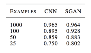
Example of the Table of Results Comparing Classification Accuracy of a CNN and SGAN on MNIST.
Taken from: Semi-Supervised Learning with Generative Adversarial Networks
Tim Salimans, et al. from OpenAI in their 2016 paper titled “Improved Techniques for Training GANs” achieved at the time state-of-the-art results on a number of image classification tasks using a semi-supervised GAN, including MNIST.
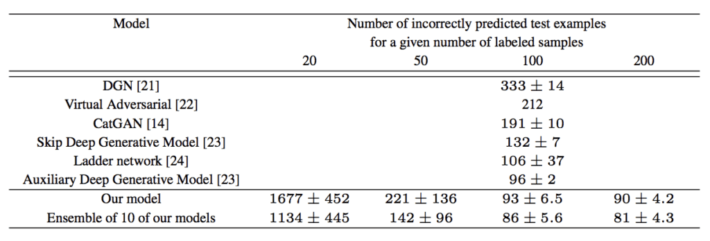
Example of the Table of Results Comparing Classification Accuracy of other GAN models to a SGAN on MNIST.
Taken From: Improved Techniques for Training GANs
Want to Develop GANs from Scratch?
Take my free 7-day email crash course now (with sample code).
Click to sign-up and also get a free PDF Ebook version of the course.
How to Implement the Semi-Supervised Discriminator Model
There are a number of ways that we can implement the discriminator model for the semi-supervised GAN.
In this section, we will review three candidate approaches.
Traditional Discriminator Model
Consider a discriminator model for the standard GAN model.
It must take an image as input and predict whether it is real or fake. More specifically, it predicts the likelihood of the input image being real. The output layer uses a sigmoid activation function to predict a probability value in [0,1] and the model is typically optimized using a binary cross entropy loss function.
For example, we can define a simple discriminator model that takes grayscale images as input with the size of 28×28 pixels and predicts a probability of the image being real. We can use best practices and downsample the image using convolutional layers with a 2×2 stride and a leaky ReLU activation function.
The define_discriminator() function below implements this and defines our standard discriminator model.
|
1 2 3 4 5 6 7 8 9 10 11 12 13 14 15 16 17 18 19 20 21 22 23 24 25 26 27 28 29 30 31 32 33 34 35 36 37 38 39 |
# example of defining the discriminator model from keras.models import Model from keras.layers import Input from keras.layers import Dense from keras.layers import Conv2D from keras.layers import LeakyReLU from keras.layers import Dropout from keras.layers import Flatten from keras.optimizers import Adam from keras.utils.vis_utils import plot_model # define the standalone discriminator model def define_discriminator(in_shape=(28,28,1)): # image input in_image = Input(shape=in_shape) # downsample fe = Conv2D(128, (3,3), strides=(2,2), padding='same')(in_image) fe = LeakyReLU(alpha=0.2)(fe) # downsample fe = Conv2D(128, (3,3), strides=(2,2), padding='same')(fe) fe = LeakyReLU(alpha=0.2)(fe) # downsample fe = Conv2D(128, (3,3), strides=(2,2), padding='same')(fe) fe = LeakyReLU(alpha=0.2)(fe) # flatten feature maps fe = Flatten()(fe) # dropout fe = Dropout(0.4)(fe) # output layer d_out_layer = Dense(1, activation='sigmoid')(fe) # define and compile discriminator model d_model = Model(in_image, d_out_layer) d_model.compile(loss='binary_crossentropy', optimizer=Adam(lr=0.0002, beta_1=0.5)) return d_model # create model model = define_discriminator() # plot the model plot_model(model, to_file='discriminator_plot.png', show_shapes=True, show_layer_names=True) |
Running the example creates a plot of the discriminator model, clearly showing the 28x28x1 shape of the input image and the prediction of a single probability value.
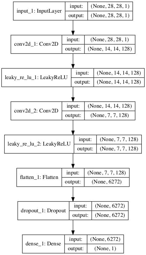
Plot of a Standard GAN Discriminator Model
Separate Discriminator Models With Shared Weights
Starting with the standard GAN discriminator model, we can update it to create two models that share feature extraction weights.
Specifically, we can define one classifier model that predicts whether an input image is real or fake, and a second classifier model that predicts the class of a given model.
- Binary Classifier Model. Predicts whether the image is real or fake, sigmoid activation function in the output layer, and optimized using the binary cross entropy loss function.
- Multi-Class Classifier Model. Predicts the class of the image, softmax activation function in the output layer, and optimized using the categorical cross entropy loss function.
Both models have different output layers but share all feature extraction layers. This means that updates to one of the classifier models will impact both models.
The example below creates the traditional discriminator model with binary output first, then re-uses the feature extraction layers and creates a new multi-class prediction model, in this case with 10 classes.
|
1 2 3 4 5 6 7 8 9 10 11 12 13 14 15 16 17 18 19 20 21 22 23 24 25 26 27 28 29 30 31 32 33 34 35 36 37 38 39 40 41 42 43 44 45 |
# example of defining semi-supervised discriminator model from keras.models import Model from keras.layers import Input from keras.layers import Dense from keras.layers import Conv2D from keras.layers import LeakyReLU from keras.layers import Dropout from keras.layers import Flatten from keras.optimizers import Adam from keras.utils.vis_utils import plot_model # define the standalone supervised and unsupervised discriminator models def define_discriminator(in_shape=(28,28,1), n_classes=10): # image input in_image = Input(shape=in_shape) # downsample fe = Conv2D(128, (3,3), strides=(2,2), padding='same')(in_image) fe = LeakyReLU(alpha=0.2)(fe) # downsample fe = Conv2D(128, (3,3), strides=(2,2), padding='same')(fe) fe = LeakyReLU(alpha=0.2)(fe) # downsample fe = Conv2D(128, (3,3), strides=(2,2), padding='same')(fe) fe = LeakyReLU(alpha=0.2)(fe) # flatten feature maps fe = Flatten()(fe) # dropout fe = Dropout(0.4)(fe) # unsupervised output d_out_layer = Dense(1, activation='sigmoid')(fe) # define and compile unsupervised discriminator model d_model = Model(in_image, d_out_layer) d_model.compile(loss='binary_crossentropy', optimizer=Adam(lr=0.0002, beta_1=0.5)) # supervised output c_out_layer = Dense(n_classes, activation='softmax')(fe) # define and compile supervised discriminator model c_model = Model(in_image, c_out_layer) c_model.compile(loss='sparse_categorical_crossentropy', optimizer=Adam(lr=0.0002, beta_1=0.5), metrics=['accuracy']) return d_model, c_model # create model d_model, c_model = define_discriminator() # plot the model plot_model(d_model, to_file='discriminator1_plot.png', show_shapes=True, show_layer_names=True) plot_model(c_model, to_file='discriminator2_plot.png', show_shapes=True, show_layer_names=True) |
Running the example creates and plots both models.
The plot for the first model is the same as before.

Plot of an Unsupervised Binary Classification GAN Discriminator Model
The plot of the second model shows the same expected input shape and same feature extraction layers, with a new 10 class classification output layer.
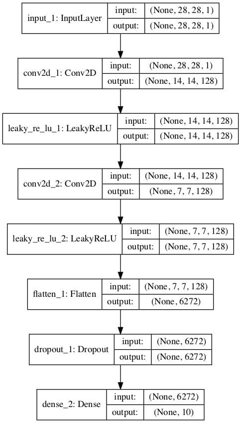
Plot of a Supervised Multi-Class Classification GAN Discriminator Model
Single Discriminator Model With Multiple Outputs
Another approach to implementing the semi-supervised discriminator model is to have a single model with multiple output layers.
Specifically, this is a single model with one output layer for the unsupervised task and one output layer for the supervised task.
This is like having separate models for the supervised and unsupervised tasks in that they both share the same feature extraction layers, except that in this case, each input image always has two output predictions, specifically a real/fake prediction and a supervised class prediction.
A problem with this approach is that when the model is updated unlabeled and generated images, there is no supervised class label. In that case, these images must have an output label of “unknown” or “fake” from the supervised output. This means that an additional class label is required for the supervised output layer.
The example below implements the multi-output single model approach for the discriminator model in the semi-supervised GAN architecture.
We can see that the model is defined with two output layers and that the output layer for the supervised task is defined with n_classes + 1. in this case 11, making room for the additional “unknown” class label.
We can also see that the model is compiled to two loss functions, one for each output layer of the model.
|
1 2 3 4 5 6 7 8 9 10 11 12 13 14 15 16 17 18 19 20 21 22 23 24 25 26 27 28 29 30 31 32 33 34 35 36 37 38 39 40 41 |
# example of defining semi-supervised discriminator model from keras.models import Model from keras.layers import Input from keras.layers import Dense from keras.layers import Conv2D from keras.layers import LeakyReLU from keras.layers import Dropout from keras.layers import Flatten from keras.optimizers import Adam from keras.utils.vis_utils import plot_model # define the standalone supervised and unsupervised discriminator models def define_discriminator(in_shape=(28,28,1), n_classes=10): # image input in_image = Input(shape=in_shape) # downsample fe = Conv2D(128, (3,3), strides=(2,2), padding='same')(in_image) fe = LeakyReLU(alpha=0.2)(fe) # downsample fe = Conv2D(128, (3,3), strides=(2,2), padding='same')(fe) fe = LeakyReLU(alpha=0.2)(fe) # downsample fe = Conv2D(128, (3,3), strides=(2,2), padding='same')(fe) fe = LeakyReLU(alpha=0.2)(fe) # flatten feature maps fe = Flatten()(fe) # dropout fe = Dropout(0.4)(fe) # unsupervised output d_out_layer = Dense(1, activation='sigmoid')(fe) # supervised output c_out_layer = Dense(n_classes + 1, activation='softmax')(fe) # define and compile supervised discriminator model model = Model(in_image, [d_out_layer, c_out_layer]) model.compile(loss=['binary_crossentropy', 'sparse_categorical_crossentropy'], optimizer=Adam(lr=0.0002, beta_1=0.5), metrics=['accuracy']) return model # create model model = define_discriminator() # plot the model plot_model(model, to_file='multioutput_discriminator_plot.png', show_shapes=True, show_layer_names=True) |
Running the example creates and plots the single multi-output model.
The plot clearly shows the shared layers and the separate unsupervised and supervised output layers.
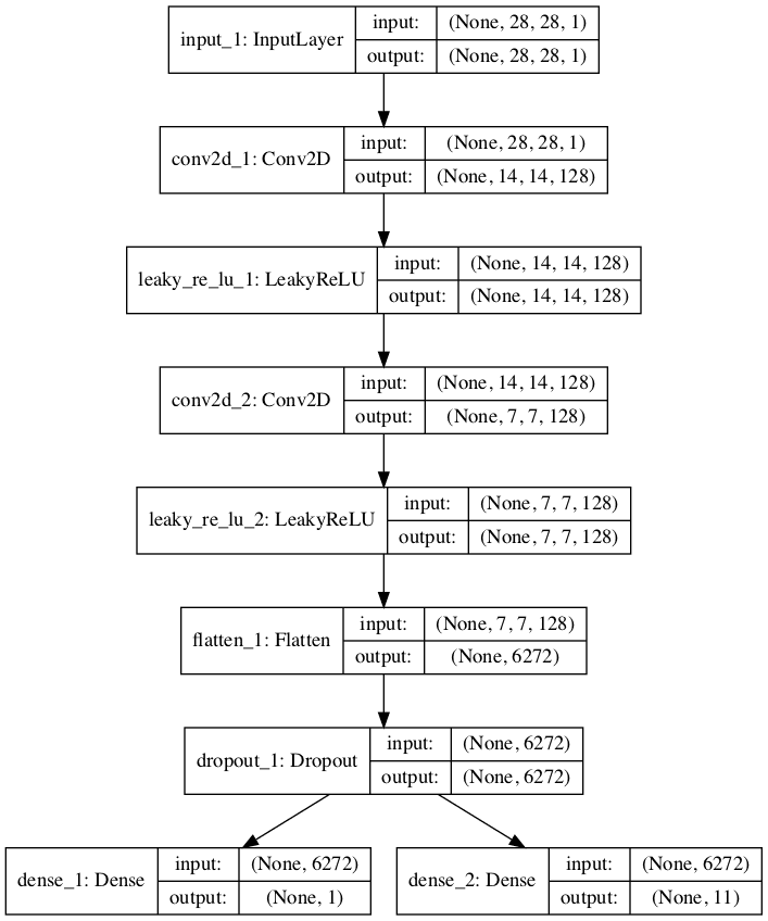
Plot of a Semi-Supervised GAN Discriminator Model With Unsupervised and Supervised Output Layers
Stacked Discriminator Models With Shared Weights
A final approach is very similar to the prior two approaches and involves creating separate logical unsupervised and supervised models but attempts to reuse the output layers of one model to feed as input into another model.
The approach is based on the definition of the semi-supervised model in the 2016 paper by Tim Salimans, et al. from OpenAI titled “Improved Techniques for Training GANs.”
In the paper, they describe an efficient implementation, where first the supervised model is created with K output classes and a softmax activation function. The unsupervised model is then defined that takes the output of the supervised model prior to the softmax activation, then calculates a normalized sum of the exponential outputs.

Example of the Output Function for the Unsupervised Discriminator Model in the SGAN.
Taken from: Improved Techniques for Training GANs
To make this clearer, we can implement this activation function in NumPy and run some sample activations through it to see what happens.
The complete example is listed below.
|
1 2 3 4 5 6 7 8 9 10 11 12 13 14 15 16 17 18 19 20 21 22 23 24 |
# example of custom activation function import numpy as np # custom activation function def custom_activation(output): logexpsum = np.sum(np.exp(output)) result = logexpsum / (logexpsum + 1.0) return result # all -10s output = np.asarray([-10.0, -10.0, -10.0]) print(custom_activation(output)) # all -1s output = np.asarray([-1.0, -1.0, -1.0]) print(custom_activation(output)) # all 0s output = np.asarray([0.0, 0.0, 0.0]) print(custom_activation(output)) # all 1s output = np.asarray([1.0, 1.0, 1.0]) print(custom_activation(output)) # all 10s output = np.asarray([10.0, 10.0, 10.0]) print(custom_activation(output)) |
Remember, the output of the unsupervised model prior to the softmax activation function will be the activations of the nodes directly. They will be small positive or negative values, but not normalized, as this would be performed by the softmax activation.
The custom activation function will output a value between 0.0 and 1.0.
A value close to 0.0 is output for a small or negative activation and a value close to 1.0 for a positive or large activation. We can see this when we run the example.
|
1 2 3 4 5 |
0.00013618124143106674 0.5246331135813284 0.75 0.890768227426964 0.9999848669190928 |
This means that the model is encouraged to output a strong class prediction for real examples, and a small class prediction or low activation for fake examples. It’s a clever trick and allows the re-use of the same output nodes from the supervised model in both models.
The activation function can be implemented almost directly via the Keras backend and called from a Lambda layer, e.g. a layer that will apply a custom function to the input to the layer.
The complete example is listed below. First, the supervised model is defined with a softmax activation and categorical cross entropy loss function. The unsupervised model is stacked on top of the output layer of the supervised model before the softmax activation, and the activations of the nodes pass through our custom activation function via the Lambda layer.
No need for a sigmoid activation function as we have already normalized the activation. As before, the unsupervised model is fit using binary cross entropy loss.
|
1 2 3 4 5 6 7 8 9 10 11 12 13 14 15 16 17 18 19 20 21 22 23 24 25 26 27 28 29 30 31 32 33 34 35 36 37 38 39 40 41 42 43 44 45 46 47 48 49 50 51 52 53 54 55 56 |
# example of defining semi-supervised discriminator model from keras.models import Model from keras.layers import Input from keras.layers import Dense from keras.layers import Conv2D from keras.layers import LeakyReLU from keras.layers import Dropout from keras.layers import Flatten from keras.layers import Activation from keras.layers import Lambda from keras.optimizers import Adam from keras.utils.vis_utils import plot_model from keras import backend # custom activation function def custom_activation(output): logexpsum = backend.sum(backend.exp(output), axis=-1, keepdims=True) result = logexpsum / (logexpsum + 1.0) return result # define the standalone supervised and unsupervised discriminator models def define_discriminator(in_shape=(28,28,1), n_classes=10): # image input in_image = Input(shape=in_shape) # downsample fe = Conv2D(128, (3,3), strides=(2,2), padding='same')(in_image) fe = LeakyReLU(alpha=0.2)(fe) # downsample fe = Conv2D(128, (3,3), strides=(2,2), padding='same')(fe) fe = LeakyReLU(alpha=0.2)(fe) # downsample fe = Conv2D(128, (3,3), strides=(2,2), padding='same')(fe) fe = LeakyReLU(alpha=0.2)(fe) # flatten feature maps fe = Flatten()(fe) # dropout fe = Dropout(0.4)(fe) # output layer nodes fe = Dense(n_classes)(fe) # supervised output c_out_layer = Activation('softmax')(fe) # define and compile supervised discriminator model c_model = Model(in_image, c_out_layer) c_model.compile(loss='sparse_categorical_crossentropy', optimizer=Adam(lr=0.0002, beta_1=0.5), metrics=['accuracy']) # unsupervised output d_out_layer = Lambda(custom_activation)(fe) # define and compile unsupervised discriminator model d_model = Model(in_image, d_out_layer) d_model.compile(loss='binary_crossentropy', optimizer=Adam(lr=0.0002, beta_1=0.5)) return d_model, c_model # create model d_model, c_model = define_discriminator() # plot the model plot_model(d_model, to_file='stacked_discriminator1_plot.png', show_shapes=True, show_layer_names=True) plot_model(c_model, to_file='stacked_discriminator2_plot.png', show_shapes=True, show_layer_names=True) |
Running the example creates and plots the two models, which look much the same as the two models in the first example.
Stacked version of the unsupervised discriminator model:
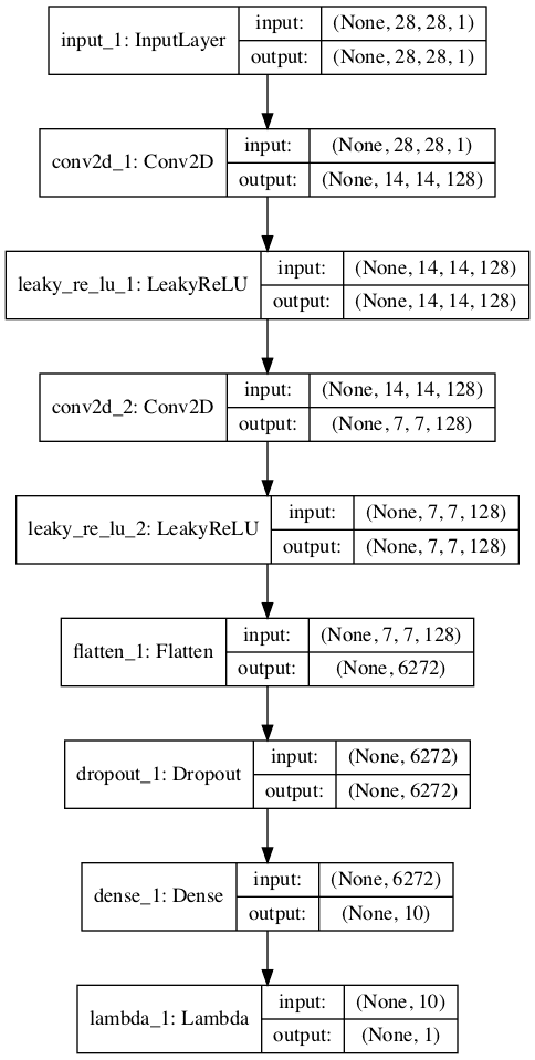
Plot of the Stacked Version of the Unsupervised Discriminator Model of the Semi-Supervised GAN
Stacked version of the supervised discriminator model:
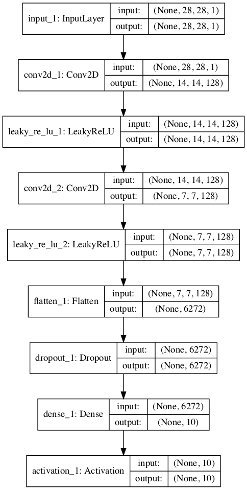
Plot of the Stacked Version of the Supervised Discriminator Model of the Semi-Supervised GAN
Now that we have seen how to implement the discriminator model in the semi-supervised GAN, we can develop a complete example for image generation and semi-supervised classification.
How to Develop a Semi-Supervised GAN for MNIST
In this section, we will develop a semi-supervised GAN model for the MNIST handwritten digit dataset.
The dataset has 10 classes for the digits 0-9, therefore the classifier model will have 10 output nodes. The model will be fit on the training dataset that contains 60,000 examples. Only 100 of the images in the training dataset will be used with labels, 10 from each of the 10 classes.
We will start off by defining the models.
We will use the stacked discriminator model, exactly as defined in the previous section.
Next, we can define the generator model. In this case, the generator model will take as input a point in the latent space and will use transpose convolutional layers to output a 28×28 grayscale image. The define_generator() function below implements this and returns the defined generator model.
|
1 2 3 4 5 6 7 8 9 10 11 12 13 14 15 16 17 18 19 20 |
# define the standalone generator model def define_generator(latent_dim): # image generator input in_lat = Input(shape=(latent_dim,)) # foundation for 7x7 image n_nodes = 128 * 7 * 7 gen = Dense(n_nodes)(in_lat) gen = LeakyReLU(alpha=0.2)(gen) gen = Reshape((7, 7, 128))(gen) # upsample to 14x14 gen = Conv2DTranspose(128, (4,4), strides=(2,2), padding='same')(gen) gen = LeakyReLU(alpha=0.2)(gen) # upsample to 28x28 gen = Conv2DTranspose(128, (4,4), strides=(2,2), padding='same')(gen) gen = LeakyReLU(alpha=0.2)(gen) # output out_layer = Conv2D(1, (7,7), activation='tanh', padding='same')(gen) # define model model = Model(in_lat, out_layer) return model |
The generator model will be fit via the unsupervised discriminator model.
We will use the composite model architecture, common to training the generator model when implemented in Keras. Specifically, weight sharing is used where the output of the generator model is passed directly to the unsupervised discriminator model, and the weights of the discriminator are marked as not trainable.
The define_gan() function below implements this, taking the already-defined generator and discriminator models as input and returning the composite model used to train the weights of the generator model.
|
1 2 3 4 5 6 7 8 9 10 11 12 |
# define the combined generator and discriminator model, for updating the generator def define_gan(g_model, d_model): # make weights in the discriminator not trainable d_model.trainable = False # connect image output from generator as input to discriminator gan_output = d_model(g_model.output) # define gan model as taking noise and outputting a classification model = Model(g_model.input, gan_output) # compile model opt = Adam(lr=0.0002, beta_1=0.5) model.compile(loss='binary_crossentropy', optimizer=opt) return model |
We can load the training dataset and scale the pixels to the range [-1, 1] to match the output values of the generator model.
|
1 2 3 4 5 6 7 8 9 10 11 12 |
# load the images def load_real_samples(): # load dataset (trainX, trainy), (_, _) = load_data() # expand to 3d, e.g. add channels X = expand_dims(trainX, axis=-1) # convert from ints to floats X = X.astype('float32') # scale from [0,255] to [-1,1] X = (X - 127.5) / 127.5 print(X.shape, trainy.shape) return [X, trainy] |
We can also define a function to select a subset of the training dataset in which we keep the labels and train the supervised version of the discriminator model.
The select_supervised_samples() function below implements this and is careful to ensure that the selection of examples is random and that the classes are balanced. The number of labeled examples is parameterized and set at 100, meaning that each of the 10 classes will have 10 randomly selected examples.
|
1 2 3 4 5 6 7 8 9 10 11 12 13 14 |
# select a supervised subset of the dataset, ensures classes are balanced def select_supervised_samples(dataset, n_samples=100, n_classes=10): X, y = dataset X_list, y_list = list(), list() n_per_class = int(n_samples / n_classes) for i in range(n_classes): # get all images for this class X_with_class = X[y == i] # choose random instances ix = randint(0, len(X_with_class), n_per_class) # add to list [X_list.append(X_with_class[j]) for j in ix] [y_list.append(i) for j in ix] return asarray(X_list), asarray(y_list) |
Next, we can define a function for retrieving a batch of real training examples.
A sample of images and labels is selected, with replacement. This same function can be used to retrieve examples from the labeled and unlabeled dataset, later when we train the models. In the case of the “unlabeled dataset“, we will ignore the labels.
|
1 2 3 4 5 6 7 8 9 10 11 |
# select real samples def generate_real_samples(dataset, n_samples): # split into images and labels images, labels = dataset # choose random instances ix = randint(0, images.shape[0], n_samples) # select images and labels X, labels = images[ix], labels[ix] # generate class labels y = ones((n_samples, 1)) return [X, labels], y |
Next, we can define functions to help in generating images using the generator model.
First, the generate_latent_points() function will create a batch worth of random points in the latent space that can be used as input for generating images. The generate_fake_samples() function will call this function to generate a batch worth of images that can be fed to the unsupervised discriminator model or the composite GAN model during training.
|
1 2 3 4 5 6 7 8 9 10 11 12 13 14 15 16 17 |
# generate points in latent space as input for the generator def generate_latent_points(latent_dim, n_samples): # generate points in the latent space z_input = randn(latent_dim * n_samples) # reshape into a batch of inputs for the network z_input = z_input.reshape(n_samples, latent_dim) return z_input # use the generator to generate n fake examples, with class labels def generate_fake_samples(generator, latent_dim, n_samples): # generate points in latent space z_input = generate_latent_points(latent_dim, n_samples) # predict outputs images = generator.predict(z_input) # create class labels y = zeros((n_samples, 1)) return images, y |
Next, we can define a function to be called when we want to evaluate the performance of the model.
This function will generate and plot 100 images using the current state of the generator model. This plot of images can be used to subjectively evaluate the performance of the generator model.
The supervised discriminator model is then evaluated on the entire training dataset, and the classification accuracy is reported. Finally, the generator model and the supervised discriminator model are saved to file, to be used later.
The summarize_performance() function below implements this and can be called periodically, such as the end of every training epoch. The results can be reviewed at the end of the run to select a classifier and even generator models.
|
1 2 3 4 5 6 7 8 9 10 11 12 13 14 15 16 17 18 19 20 21 22 23 24 25 26 27 28 29 |
# generate samples and save as a plot and save the model def summarize_performance(step, g_model, c_model, latent_dim, dataset, n_samples=100): # prepare fake examples X, _ = generate_fake_samples(g_model, latent_dim, n_samples) # scale from [-1,1] to [0,1] X = (X + 1) / 2.0 # plot images for i in range(100): # define subplot pyplot.subplot(10, 10, 1 + i) # turn off axis pyplot.axis('off') # plot raw pixel data pyplot.imshow(X[i, :, :, 0], cmap='gray_r') # save plot to file filename1 = 'generated_plot_%04d.png' % (step+1) pyplot.savefig(filename1) pyplot.close() # evaluate the classifier model X, y = dataset _, acc = c_model.evaluate(X, y, verbose=0) print('Classifier Accuracy: %.3f%%' % (acc * 100)) # save the generator model filename2 = 'g_model_%04d.h5' % (step+1) g_model.save(filename2) # save the classifier model filename3 = 'c_model_%04d.h5' % (step+1) c_model.save(filename3) print('>Saved: %s, %s, and %s' % (filename1, filename2, filename3)) |
Next, we can define a function to train the models. The defined models and loaded training dataset are provided as arguments, and the number of training epochs and batch size are parameterized with default values, in this case 20 epochs and a batch size of 100.
The chosen model configuration was found to overfit the training dataset quickly, hence the relatively smaller number of training epochs. Increasing the epochs to 100 or more results in much higher-quality generated images, but a lower-quality classifier model. Balancing these two concerns might make a fun extension.
First, the labeled subset of the training dataset is selected, and the number of training steps is calculated.
The training process is almost identical to the training of a vanilla GAN model, with the addition of updating the supervised model with labeled examples.
A single cycle through updating the models involves first updating the supervised discriminator model with labeled examples, then updating the unsupervised discriminator model with unlabeled real and generated examples. Finally, the generator model is updated via the composite model.
The shared weights of the discriminator model get updated with 1.5 batches worth of samples, whereas the weights of the generator model are updated with one batch worth of samples each iteration. Changing this so that each model is updated by the same amount might improve the model training process.
|
1 2 3 4 5 6 7 8 9 10 11 12 13 14 15 16 17 18 19 20 21 22 23 24 25 26 27 28 29 30 |
# train the generator and discriminator def train(g_model, d_model, c_model, gan_model, dataset, latent_dim, n_epochs=20, n_batch=100): # select supervised dataset X_sup, y_sup = select_supervised_samples(dataset) print(X_sup.shape, y_sup.shape) # calculate the number of batches per training epoch bat_per_epo = int(dataset[0].shape[0] / n_batch) # calculate the number of training iterations n_steps = bat_per_epo * n_epochs # calculate the size of half a batch of samples half_batch = int(n_batch / 2) print('n_epochs=%d, n_batch=%d, 1/2=%d, b/e=%d, steps=%d' % (n_epochs, n_batch, half_batch, bat_per_epo, n_steps)) # manually enumerate epochs for i in range(n_steps): # update supervised discriminator (c) [Xsup_real, ysup_real], _ = generate_real_samples([X_sup, y_sup], half_batch) c_loss, c_acc = c_model.train_on_batch(Xsup_real, ysup_real) # update unsupervised discriminator (d) [X_real, _], y_real = generate_real_samples(dataset, half_batch) d_loss1 = d_model.train_on_batch(X_real, y_real) X_fake, y_fake = generate_fake_samples(g_model, latent_dim, half_batch) d_loss2 = d_model.train_on_batch(X_fake, y_fake) # update generator (g) X_gan, y_gan = generate_latent_points(latent_dim, n_batch), ones((n_batch, 1)) g_loss = gan_model.train_on_batch(X_gan, y_gan) # summarize loss on this batch print('>%d, c[%.3f,%.0f], d[%.3f,%.3f], g[%.3f]' % (i+1, c_loss, c_acc*100, d_loss1, d_loss2, g_loss)) # evaluate the model performance every so often if (i+1) % (bat_per_epo * 1) == 0: summarize_performance(i, g_model, c_model, latent_dim, dataset) |
Finally, we can define the models and call the function to train and save the models.
|
1 2 3 4 5 6 7 8 9 10 11 12 |
# size of the latent space latent_dim = 100 # create the discriminator models d_model, c_model = define_discriminator() # create the generator g_model = define_generator(latent_dim) # create the gan gan_model = define_gan(g_model, d_model) # load image data dataset = load_real_samples() # train model train(g_model, d_model, c_model, gan_model, dataset, latent_dim) |
Tying all of this together, the complete example of training a semi-supervised GAN on the MNIST handwritten digit image classification task is listed below.
|
1 2 3 4 5 6 7 8 9 10 11 12 13 14 15 16 17 18 19 20 21 22 23 24 25 26 27 28 29 30 31 32 33 34 35 36 37 38 39 40 41 42 43 44 45 46 47 48 49 50 51 52 53 54 55 56 57 58 59 60 61 62 63 64 65 66 67 68 69 70 71 72 73 74 75 76 77 78 79 80 81 82 83 84 85 86 87 88 89 90 91 92 93 94 95 96 97 98 99 100 101 102 103 104 105 106 107 108 109 110 111 112 113 114 115 116 117 118 119 120 121 122 123 124 125 126 127 128 129 130 131 132 133 134 135 136 137 138 139 140 141 142 143 144 145 146 147 148 149 150 151 152 153 154 155 156 157 158 159 160 161 162 163 164 165 166 167 168 169 170 171 172 173 174 175 176 177 178 179 180 181 182 183 184 185 186 187 188 189 190 191 192 193 194 195 196 197 198 199 200 201 202 203 204 205 206 207 208 209 210 211 212 213 214 215 216 217 218 219 220 221 222 223 224 225 |
# example of semi-supervised gan for mnist from numpy import expand_dims from numpy import zeros from numpy import ones from numpy import asarray from numpy.random import randn from numpy.random import randint from keras.datasets.mnist import load_data from keras.optimizers import Adam from keras.models import Model from keras.layers import Input from keras.layers import Dense from keras.layers import Reshape from keras.layers import Flatten from keras.layers import Conv2D from keras.layers import Conv2DTranspose from keras.layers import LeakyReLU from keras.layers import Dropout from keras.layers import Lambda from keras.layers import Activation from matplotlib import pyplot from keras import backend # custom activation function def custom_activation(output): logexpsum = backend.sum(backend.exp(output), axis=-1, keepdims=True) result = logexpsum / (logexpsum + 1.0) return result # define the standalone supervised and unsupervised discriminator models def define_discriminator(in_shape=(28,28,1), n_classes=10): # image input in_image = Input(shape=in_shape) # downsample fe = Conv2D(128, (3,3), strides=(2,2), padding='same')(in_image) fe = LeakyReLU(alpha=0.2)(fe) # downsample fe = Conv2D(128, (3,3), strides=(2,2), padding='same')(fe) fe = LeakyReLU(alpha=0.2)(fe) # downsample fe = Conv2D(128, (3,3), strides=(2,2), padding='same')(fe) fe = LeakyReLU(alpha=0.2)(fe) # flatten feature maps fe = Flatten()(fe) # dropout fe = Dropout(0.4)(fe) # output layer nodes fe = Dense(n_classes)(fe) # supervised output c_out_layer = Activation('softmax')(fe) # define and compile supervised discriminator model c_model = Model(in_image, c_out_layer) c_model.compile(loss='sparse_categorical_crossentropy', optimizer=Adam(lr=0.0002, beta_1=0.5), metrics=['accuracy']) # unsupervised output d_out_layer = Lambda(custom_activation)(fe) # define and compile unsupervised discriminator model d_model = Model(in_image, d_out_layer) d_model.compile(loss='binary_crossentropy', optimizer=Adam(lr=0.0002, beta_1=0.5)) return d_model, c_model # define the standalone generator model def define_generator(latent_dim): # image generator input in_lat = Input(shape=(latent_dim,)) # foundation for 7x7 image n_nodes = 128 * 7 * 7 gen = Dense(n_nodes)(in_lat) gen = LeakyReLU(alpha=0.2)(gen) gen = Reshape((7, 7, 128))(gen) # upsample to 14x14 gen = Conv2DTranspose(128, (4,4), strides=(2,2), padding='same')(gen) gen = LeakyReLU(alpha=0.2)(gen) # upsample to 28x28 gen = Conv2DTranspose(128, (4,4), strides=(2,2), padding='same')(gen) gen = LeakyReLU(alpha=0.2)(gen) # output out_layer = Conv2D(1, (7,7), activation='tanh', padding='same')(gen) # define model model = Model(in_lat, out_layer) return model # define the combined generator and discriminator model, for updating the generator def define_gan(g_model, d_model): # make weights in the discriminator not trainable d_model.trainable = False # connect image output from generator as input to discriminator gan_output = d_model(g_model.output) # define gan model as taking noise and outputting a classification model = Model(g_model.input, gan_output) # compile model opt = Adam(lr=0.0002, beta_1=0.5) model.compile(loss='binary_crossentropy', optimizer=opt) return model # load the images def load_real_samples(): # load dataset (trainX, trainy), (_, _) = load_data() # expand to 3d, e.g. add channels X = expand_dims(trainX, axis=-1) # convert from ints to floats X = X.astype('float32') # scale from [0,255] to [-1,1] X = (X - 127.5) / 127.5 print(X.shape, trainy.shape) return [X, trainy] # select a supervised subset of the dataset, ensures classes are balanced def select_supervised_samples(dataset, n_samples=100, n_classes=10): X, y = dataset X_list, y_list = list(), list() n_per_class = int(n_samples / n_classes) for i in range(n_classes): # get all images for this class X_with_class = X[y == i] # choose random instances ix = randint(0, len(X_with_class), n_per_class) # add to list [X_list.append(X_with_class[j]) for j in ix] [y_list.append(i) for j in ix] return asarray(X_list), asarray(y_list) # select real samples def generate_real_samples(dataset, n_samples): # split into images and labels images, labels = dataset # choose random instances ix = randint(0, images.shape[0], n_samples) # select images and labels X, labels = images[ix], labels[ix] # generate class labels y = ones((n_samples, 1)) return [X, labels], y # generate points in latent space as input for the generator def generate_latent_points(latent_dim, n_samples): # generate points in the latent space z_input = randn(latent_dim * n_samples) # reshape into a batch of inputs for the network z_input = z_input.reshape(n_samples, latent_dim) return z_input # use the generator to generate n fake examples, with class labels def generate_fake_samples(generator, latent_dim, n_samples): # generate points in latent space z_input = generate_latent_points(latent_dim, n_samples) # predict outputs images = generator.predict(z_input) # create class labels y = zeros((n_samples, 1)) return images, y # generate samples and save as a plot and save the model def summarize_performance(step, g_model, c_model, latent_dim, dataset, n_samples=100): # prepare fake examples X, _ = generate_fake_samples(g_model, latent_dim, n_samples) # scale from [-1,1] to [0,1] X = (X + 1) / 2.0 # plot images for i in range(100): # define subplot pyplot.subplot(10, 10, 1 + i) # turn off axis pyplot.axis('off') # plot raw pixel data pyplot.imshow(X[i, :, :, 0], cmap='gray_r') # save plot to file filename1 = 'generated_plot_%04d.png' % (step+1) pyplot.savefig(filename1) pyplot.close() # evaluate the classifier model X, y = dataset _, acc = c_model.evaluate(X, y, verbose=0) print('Classifier Accuracy: %.3f%%' % (acc * 100)) # save the generator model filename2 = 'g_model_%04d.h5' % (step+1) g_model.save(filename2) # save the classifier model filename3 = 'c_model_%04d.h5' % (step+1) c_model.save(filename3) print('>Saved: %s, %s, and %s' % (filename1, filename2, filename3)) # train the generator and discriminator def train(g_model, d_model, c_model, gan_model, dataset, latent_dim, n_epochs=20, n_batch=100): # select supervised dataset X_sup, y_sup = select_supervised_samples(dataset) print(X_sup.shape, y_sup.shape) # calculate the number of batches per training epoch bat_per_epo = int(dataset[0].shape[0] / n_batch) # calculate the number of training iterations n_steps = bat_per_epo * n_epochs # calculate the size of half a batch of samples half_batch = int(n_batch / 2) print('n_epochs=%d, n_batch=%d, 1/2=%d, b/e=%d, steps=%d' % (n_epochs, n_batch, half_batch, bat_per_epo, n_steps)) # manually enumerate epochs for i in range(n_steps): # update supervised discriminator (c) [Xsup_real, ysup_real], _ = generate_real_samples([X_sup, y_sup], half_batch) c_loss, c_acc = c_model.train_on_batch(Xsup_real, ysup_real) # update unsupervised discriminator (d) [X_real, _], y_real = generate_real_samples(dataset, half_batch) d_loss1 = d_model.train_on_batch(X_real, y_real) X_fake, y_fake = generate_fake_samples(g_model, latent_dim, half_batch) d_loss2 = d_model.train_on_batch(X_fake, y_fake) # update generator (g) X_gan, y_gan = generate_latent_points(latent_dim, n_batch), ones((n_batch, 1)) g_loss = gan_model.train_on_batch(X_gan, y_gan) # summarize loss on this batch print('>%d, c[%.3f,%.0f], d[%.3f,%.3f], g[%.3f]' % (i+1, c_loss, c_acc*100, d_loss1, d_loss2, g_loss)) # evaluate the model performance every so often if (i+1) % (bat_per_epo * 1) == 0: summarize_performance(i, g_model, c_model, latent_dim, dataset) # size of the latent space latent_dim = 100 # create the discriminator models d_model, c_model = define_discriminator() # create the generator g_model = define_generator(latent_dim) # create the gan gan_model = define_gan(g_model, d_model) # load image data dataset = load_real_samples() # train model train(g_model, d_model, c_model, gan_model, dataset, latent_dim) |
The example can be run on a workstation with a CPU or GPU hardware, although a GPU is recommended for faster execution.
Note: Your results may vary given the stochastic nature of the algorithm or evaluation procedure, or differences in numerical precision. Consider running the example a few times and compare the average outcome.
At the start of the run, the size of the training dataset is summarized, as is the supervised subset, confirming our configuration.
The performance of each model is summarized at the end of each update, including the loss and accuracy of the supervised discriminator model (c), the loss of the unsupervised discriminator model on real and generated examples (d), and the loss of the generator model updated via the composite model (g).
The loss for the supervised model will shrink to a small value close to zero and accuracy will hit 100%, which will be maintained for the entire run. The loss of the unsupervised discriminator and generator should remain at modest values throughout the run if they are kept in equilibrium.
|
1 2 3 4 5 6 7 8 9 |
(60000, 28, 28, 1) (60000,) (100, 28, 28, 1) (100,) n_epochs=20, n_batch=100, 1/2=50, b/e=600, steps=12000 >1, c[2.305,6], d[0.096,2.399], g[0.095] >2, c[2.298,18], d[0.089,2.399], g[0.095] >3, c[2.308,10], d[0.084,2.401], g[0.095] >4, c[2.304,8], d[0.080,2.404], g[0.095] >5, c[2.254,18], d[0.077,2.407], g[0.095] ... |
The supervised classification model is evaluated on the entire training dataset at the end of every training epoch, in this case after every 600 training updates. At this time, the performance of the model is summarized, showing that it rapidly achieves good skill.
This is surprising given that the model is only trained on 10 labeled examples of each class.
|
1 2 3 4 5 6 7 8 9 10 11 12 13 14 15 16 17 18 19 20 |
Classifier Accuracy: 85.543% Classifier Accuracy: 91.487% Classifier Accuracy: 92.628% Classifier Accuracy: 94.017% Classifier Accuracy: 94.252% Classifier Accuracy: 93.828% Classifier Accuracy: 94.122% Classifier Accuracy: 93.597% Classifier Accuracy: 95.283% Classifier Accuracy: 95.287% Classifier Accuracy: 95.263% Classifier Accuracy: 95.432% Classifier Accuracy: 95.270% Classifier Accuracy: 95.212% Classifier Accuracy: 94.803% Classifier Accuracy: 94.640% Classifier Accuracy: 93.622% Classifier Accuracy: 91.870% Classifier Accuracy: 92.525% Classifier Accuracy: 92.180% |
The models are also saved at the end of each training epoch and plots of generated images are also created.
The quality of the generated images is good given the relatively small number of training epochs.
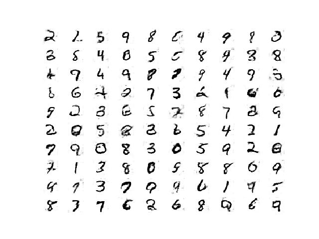
Plot of Handwritten Digits Generated by the Semi-Supervised GAN After 8400 Updates.
How to Load and Use the Final SGAN Classifier Model
Now that we have trained the generator and discriminator models, we can make use of them.
In the case of the semi-supervised GAN, we are less interested in the generator model and more interested in the supervised model.
Reviewing the results for the specific run, we can select a specific saved model that is known to have good performance on the test dataset. In this case, the model saved after 12 training epochs, or 7,200 updates, that had a classification accuracy of about 95.432% on the training dataset.
We can load the model directly via the load_model() Keras function.
|
1 2 3 |
... # load the model model = load_model('c_model_7200.h5') |
Once loaded, we can evaluate it on the entire training dataset again to confirm the finding, then evaluate it on the holdout test dataset.
Recall, the feature extraction layers expect the input images to have the pixel values scaled to the range [-1,1], therefore, this must be performed before any images are provided to the model.
The complete example of loading the saved semi-supervised classifier model and evaluating it in the complete MNIST dataset is listed below.
|
1 2 3 4 5 6 7 8 9 10 11 12 13 14 15 16 17 18 19 20 21 22 |
# example of loading the classifier model and generating images from numpy import expand_dims from keras.models import load_model from keras.datasets.mnist import load_data # load the model model = load_model('c_model_7200.h5') # load the dataset (trainX, trainy), (testX, testy) = load_data() # expand to 3d, e.g. add channels trainX = expand_dims(trainX, axis=-1) testX = expand_dims(testX, axis=-1) # convert from ints to floats trainX = trainX.astype('float32') testX = testX.astype('float32') # scale from [0,255] to [-1,1] trainX = (trainX - 127.5) / 127.5 testX = (testX - 127.5) / 127.5 # evaluate the model _, train_acc = model.evaluate(trainX, trainy, verbose=0) print('Train Accuracy: %.3f%%' % (train_acc * 100)) _, test_acc = model.evaluate(testX, testy, verbose=0) print('Test Accuracy: %.3f%%' % (test_acc * 100)) |
Running the example loads the model and evaluates it on the MNIST dataset.
Note: Your results may vary given the stochastic nature of the algorithm or evaluation procedure, or differences in numerical precision. Consider running the example a few times and compare the average outcome.
We can see that, in this case, the model achieves the expected performance of 95.432% on the training dataset, confirming we have loaded the correct model.
We can also see that the accuracy on the holdout test dataset is as good, or slightly better, at about 95.920%. This shows that the learned classifier has good generalization.
|
1 2 |
Train Accuracy: 95.432% Test Accuracy: 95.920% |
We have successfully demonstrated the training and evaluation of a semi-supervised classifier model fit via the GAN architecture.
Extensions
This section lists some ideas for extending the tutorial that you may wish to explore.
- Standalone Classifier. Fit a standalone classifier model on the labeled dataset directly and compare performance to the SGAN model.
- Number of Labeled Examples. Repeat the example of more or fewer labeled examples and compare the performance of the model
- Model Tuning. Tune the performance of the discriminator and generator model to further lift the performance of the supervised model closer toward state-of-the-art results.
If you explore any of these extensions, I’d love to know.
Post your findings in the comments below.
Further Reading
This section provides more resources on the topic if you are looking to go deeper.
Papers
- Semi-Supervised Learning with Generative Adversarial Networks, 2016.
- Improved Techniques for Training GANs, 2016.
- Unsupervised and Semi-supervised Learning with Categorical Generative Adversarial Networks, 2015.
- Semi-supervised Learning with GANs: Manifold Invariance with Improved Inference, 2017.
- Semi-Supervised Learning with GANs: Revisiting Manifold Regularization, 2018.
API
- Keras Datasets API.
- Keras Sequential Model API
- Keras Convolutional Layers API
- How can I “freeze” Keras layers?
- MatplotLib API
- NumPy Random sampling (numpy.random) API
- NumPy Array manipulation routines
Articles
- Semi-supervised learning with GANs, 2018.
- Semi-supervised learning with Generative Adversarial Networks (GANs), 2017.
Projects
- Improved GAN Project (Official), GitHub.
- Keras GAN Project, GitHub.
- GAN for semi-supervised learning Project, GitHub
Summary
In this tutorial, you discovered how to develop a Semi-Supervised Generative Adversarial Network from scratch.
Specifically, you learned:
- The semi-supervised GAN is an extension of the GAN architecture for training a classifier model while making use of labeled and unlabeled data.
- There are at least three approaches to implementing the supervised and unsupervised discriminator models in Keras used in the semi-supervised GAN.
- How to train a semi-supervised GAN from scratch on MNIST and load and use the trained classifier for making predictions.
Do you have any questions?
Ask your questions in the comments below and I will do my best to answer.




The concept of SGAN is very well explained. Can you please incorporate feature matching in the above code?
Thanks for the suggestion. Perhaps in the future.
Hi there! I just implement a possible feature matching version. But I find FM trick didn’t help at all. Any advice? My code is here:
https://github.com/King-Of-Knights/Keras-Semi-Supervised-Learning-GANs/blob/master/sslgan_feature_match.py
Nice work.
Sorry, I don’t have the capacity to review debug code as I get a ton of similar requests daily:
https://machinelearningmastery.com/faq/single-faq/can-you-read-review-or-debug-my-code
Thanks Jason for the nice explanation. I ran the code, it took a long time of execution.
Do you think with this long time of execution, SGAN can compete with other types of semi-supervised learning such as VAT
Well done!
It really depends on the specifics of the problem and the models. It is a good idea to test a range of methods.
Excellent Jason! But what if instead of custom_activation function I needed to use a custom function which was not included in backend. For example, I generated a face image as output and I want to calculate its FaceNet embedding and penalize the dissimilarity between those of the generated and the actual in my loss function. I thought I could change it to an array using tf.session.run and then calculate its FaceNet embedding but it threw the error that I must feed a value for placeholder tensor.
Very cool idea!
You can use custom functions, but recall you will be working with tensors, not arrays. Therefore all simple operations will have to use functions from backend that will wrap TF/Theano functions for tensors.
Some experimentation may be required.
You mean I need to change all the code of Facenet predict? Or if I want to use dlib to extract 68 landmarks for each tensor I need to change their code. In their code they clearly said it supports either list or array as input. There’s no other way to get around this?
No, I meant that if you use a custom function you will be working with tensors not arrays.
what are the versions of keras and tensorflow that you use?
Keras 2.3 and TF2.0.
# update supervised discriminator (c)
[Xsup_real, ysup_real], _ = generate_real_samples([X_sup, y_sup], half_batch)
c_loss, c_acc = c_model.train_on_batch(Xsup_real, ysup_real)
If we want to train the supervised discriminator, we need to use labeled data right? I mean we should use:
[Xsup_real, ysup_real], _ = select_supervised_samples(datasets)
rather than
[Xsup_real, ysup_real], _ = generate_real_samples([X_sup, y_sup], half_batch)
I am confused, am I wrong? Thanks!
I am sorry it was my fault, never mind! Your tutorial is awesome, really helps me a lot!
No problem.
est ce que vous pouvez nous prposer un tuto sur la CatGAN
Thanks for the suggestion!
Thank you for the great explanations!
I want to play with your SGAN code for the segmentation of 2d images.
Since I am new to deep learning, so I want to ask some questions.
1. Modification of the current 1d output layer of discriminator to the 2d output layer will work for the segmentation?
2. If you know, could you tell me any good example of Keras segmentation code for 2d images?
3. What would you do if you modify your code for segmentation of 2d images?
Thank you again and have a nice day!
Sorry, I don’t know how to adapt this example for segmentation directly.
Thanks for an amazing article!
I looked at two extensions that you wrote about and compaired the SGAN performances to a standalone classifier. I trained the SGAN and the standalone classifier on a different number of labeled data each time.
I also added augmentation to the standalone classifier and to the SGAN (mainly because the standalone classifier had very low perfomances without data augmentation).
The results are pretty much as expected but really show the impact of the SGAN with little supervised data.
The code and the results ( generated graphs) are available via my github repo – https://github.com/zoharri/SGAN_vs_Classifier.
Thanks.
Well done on your extensions! Thanks for sharing.
Hi Json, Thanks for the explanation.
Discriminator multi-classifier instance in SGAN is trained independently and not connected with generator. Could you please explain How it is different from plain CNN classifier?
The discriminator is a simple image classifier.
Thanks for the great article!
I am getting confused about how to feed the input to the Single Discriminator Model With Multiple Outputs. Let’s say we have X_train (labeled) and X_test(unlabeled) data. The output of the X_test should be given of ” d_output_layer ” and the output of the X_train should be given of ” c_output_layer”. So, how we can handle that. I mean how to feed data and get output from the desired layer.
Thanks
Sorry, I don’t follow the problem you’re having.
Which python, keras and tensorflow version is suitable to run the above code.
i got the following error for python 3.6
ImportError: Could not find ‘msvcp140.dll’. TensorFlow requires that this DLL be installed in a directory that is named in your %PATH% environment variable. You may install this DLL by downloading Visual C++ 2015 Redistributable Update 3 from this URL: https://www.microsoft.com/en-us/download/details.aspx?id=53587
Keras 2.3 and TensorFlow 2.
Thanks for taking out your precious time to clear my doubts.
You’re welcome.
Hi Jason,
Thank you for this amazing tutorial.
I tried to implement it for my use case, but the generator is generating the same image for all the classes. Do you have any idea why this could happen?
You’re welcome.
Perhaps try changing the configuration of the model for your data?
I did try increasing the number of samples per class. Is there any other parameter I should change that can plausibly improve this situation?
Yes, see this:
https://machinelearningmastery.com/how-to-code-generative-adversarial-network-hacks/
Hi! Thanks for explaining it so well !
I have a question regarding stacked discriminator with shared weights. If both supervised and unsupervised discriminator are sharing weights before activation layer. How come c_model has 316,938 weights but d_model has 633,876 weights? It looks like to me that c_model and d_model are both sharing common layers and applying different activation functions to create different models. So should they not have the same number of weights?
Thank you!
Sorry! I meant 316,938 parameters and 633,876 parameters, not weights.
Perhaps this will help in understanding GAN training:
https://machinelearningmastery.com/how-to-code-the-generative-adversarial-network-training-algorithm-and-loss-functions/
Hi,
A great article, I was able to implement this for my application. I am confused that which model should I save to generate images?. How are you generating images in the last? Which model should I save to do the same? In general, we save the generator model but here I am confused.
Thanks 🙂
Thanks!
The generator model is used for generating images.
Yes, we save the generator model.
Hi, Your article is so good and is helpful for me !
I have a little question that if this model can be transformed into the conventional data which is in the form of vector , and how to change it?
Thanks!
Thanks!
Yes, but GANs are intended for images, not tabular data. Here’s an example:
https://machinelearningmastery.com/how-to-develop-a-generative-adversarial-network-for-a-1-dimensional-function-from-scratch-in-keras/
What is meant by classifier accuracy in this tutorial. Is this meant that how efficiently classifier is identifying samples label i.e.among 0-9. Or classifier accuracy denotes how efficiently classifier differentiate between real and generated (or fake) samples. Further, is classifier accuracy and train accuracy is same.
Here we are training a generator and a classification model. Accuracy refers to the classification model.
Perhaps re-read the section “What Is the Semi-Supervised GAN?”
How to get class labels of images generated by generator.
You could classify the generated images with the classification model.
Thanks, this line will work for me “c_out_layer = Activation(‘softmax’)(fe)”
Nice!
how to choose the latent_dim? and does the value belong to the dataset?
I’m trying to apply this on a different dataset, so how to adjust the value of laten_dim on another dataset? because I used value = 100 and gave me a bad accuracy of 53%, or is it another problem?
Thanks,
Often small. Models are not very sensitive to the size as they impose their own structure.
Thanks, I’m actually trying your code on my data with images of size 256x256x3 and I’m getting low accuracy, so I was wondering if the problem has to do with the classification model or with the latent dimension because I also displayed the generated images and they have very poor quality after many iterations?
Accuracy is a poor metric for GANs, loot at the generated images directly.
Perhaps some of the tips here will help:
https://machinelearningmastery.com/how-to-code-generative-adversarial-network-hacks/
You said training beyond 100 epochs will improve image generation but not classification (on example in epoch 12 reached highest classifier acc.) and now you are arguing that image quality is important for accuracy? Wheres the catch? ???? Could you give more insights over accuracy vs image generation please? Btw awesome works all around this page you rock, thanks and keep it up!
Sorry, my comment was generic for GANs, e.g. when using GANs for image generation.
Hi
Great article, I learned a lot.
One thing that isn’t clear to me. When training the generator, why do you genrate labels as 1’s:
X_gan, y_gan = generate_latent_points(latent_dim, n_batch), ones((n_batch, 1))
Good question, see this:
https://machinelearningmastery.com/how-to-code-the-generative-adversarial-network-training-algorithm-and-loss-functions/
Hi Jason,
Thank you very much for the clear and useful article!
I have ran into a weird issue though when adapting this example in tensorflow (2.3.0) – the model gets trained to a reasonable accuracy even in a single epoch/600 steps, but if I save and then load it back, I end up with random accuracy (~10%).
Do you have any idea what may be the problem?
…
# train model
train(g_model, d_model, c_model, gan_model, dataset, latent_dim, n_epochs=1)
# load the dataset
(trainX, trainy) = dataset
_, train_acc = c_model.evaluate(trainX, trainy, verbose=0)
print(‘Final Accuracy: %.3f%%’ % (train_acc * 100)) # this is >80%
### load c_model from file and apply to same data:
from tensorflow.keras.models import load_model
model = load_model(‘res/c_model_0600_sm’) #.h5
_, train_acc = model.evaluate(trainX, trainy, verbose=0)
print(‘Final Accuracy: %.3f%%’ % (train_acc * 100)) # this is <10%
Perhaps try using the standalone Keras library and compare results on your system?
Hi Jason
Thank you very much for your passion for ML and your useful articles
I faced the same issue in google colab. what do you mean by “using the standalone Keras library”?
I think even when you import keras library, colab automatically imports tensorflow.keras and the version of tensorflow is 2.3.0. I did some search and understood none. would you please help.
Thanks
I meant use keras not tf.keras:
https://machinelearningmastery.com/faq/single-faq/what-is-the-difference-between-keras-and-tf-keras
Hello!
Why did we set the d_model.trainable to False? I thought we train the d_model, and disable the generator in Semi-supervised Gan.
Thank you in advance!
Good question, you can learn more about how we construct the GAN models in Keras for training here:
https://machinelearningmastery.com/how-to-code-the-generative-adversarial-network-training-algorithm-and-loss-functions/
Thank you!
Hey Jason,
Thanks for this great explanation!
– Can you please introduce articles/resources for “self-supervised image classification using CNN”?
Consider that our dataset does not have any labels (annotated labels) and we want to classify its images. What would be your solution?
Thanks for your guidance,
Thanks for the suggestion.
Do you know any resource I can refer to?
Thanks
Yes, this will help:
https://machinelearningmastery.com/faq/single-faq/where-can-i-get-a-research-paper-on-___
Hello, can you give an architecture image like this one -> https://media.arxiv-vanity.com/render-output/3592810/semi_gans.png
Thank you!
Thanks for the suggestion.
Hello, I really find this concept very interesting. However, I am trying to run the code to have a visual experience but there seem to be some error messages. Also, I want to find out if the SGAN will be viable for the classification of real and fake fingerprints because I am currently working on that. Thanks
Thanks.
Why not use a multilayer perceptron model directly? Why use a GAN?
Hi Jason,
I implement your code. But I don’t know why when I load model and test model, accuracy is 9.99%.
Perhaps double check you copied all of the code exactly?
Perhaps try refitting the model?
Perhaps check library version numbers?
this is process training:
>11988, c[0.001,100], d[0.742,0.858], g[1.056]
>11989, c[0.001,100], d[0.828,0.937], g[0.922]
>11990, c[0.001,100], d[0.970,0.843], g[0.903]
>11991, c[0.001,100], d[0.792,0.848], g[1.147]
>11992, c[0.001,100], d[0.944,0.992], g[1.223]
>11993, c[0.002,100], d[0.712,0.919], g[1.263]
>11994, c[0.002,100], d[0.667,0.846], g[1.177]
>11995, c[0.002,100], d[0.923,0.911], g[1.162]
>11996, c[0.001,100], d[0.916,0.775], g[1.115]
>11997, c[0.001,100], d[0.799,0.638], g[0.975]
>11998, c[0.002,100], d[0.837,0.939], g[0.914]
>11999, c[0.001,100], d[0.810,0.816], g[0.961]
>12000, c[0.001,100], d[0.676,0.928], g[1.012]
Classifier Accuracy: 92.422%
>Saved: generated_plot_12000.png, g_model_12000.h5, and c_model_12000.h5
But when I load model, this is results
WARNING:tensorflow:Error in loading the saved optimizer state. As a result, your model is starting with a freshly initialized optimizer.
Train Accuracy: 9.690%
Test Accuracy: 9.720%
Hi Sir,
I would like to thank you for your response,
I run your code with MNIST dataset, it is exactly raw by raw and the Accuracy when training is correct with high accuracy, but after I load the model and test it is different. I am not sure what is reason. When I try with another dataset, I also meet a similar error.
That is very odd! I have not seen that before.
I wonder if the model is not being saved/loaded correctly, e.g. perhaps check weight values before and after.
Hi, Thank you so much for your comment.
I check the TensorFlow and Keras and now the results are ok.
Thank you so much again.
Hello, when you set d_model.trainable = False, doesn’t that prevent the discriminator from learning? Maybe train_on_batch overrides this, but I’m trying this with tf.gradienttape and unless I turn d_model.trainable to True mid training, I cant change the weights on the model.
No.
It only takes effect in the composite model. You can learn more about layer freezing in the API documentation.
You can still manually change weights – the “trainable” flag is respected internal by the Keras API in calls to fit() etc.
Hello,
By setting d_model.trainable = False, doesn’t that keep both the discriminator and classifier from learning? At least I tried it using GradientTape. Maybe train_on_batch overrides that?Am I understanding something wrong?
No. It only impacts the discriminator when it is part composite model.
Perhaps start here:
https://machinelearningmastery.com/how-to-develop-a-generative-adversarial-network-for-a-1-dimensional-function-from-scratch-in-keras/
How to load data incase of custom dataset? Suppose, I previously have a dataset of images in my machine.
Perhaps this will help you load images:
https://machinelearningmastery.com/how-to-load-and-manipulate-images-for-deep-learning-in-python-with-pil-pillow/
I didn’t understand what actually latent space is?
Yeah, I hear you. It’s a little crazy first time.
Try this tutorial:
https://machinelearningmastery.com/what-are-generative-adversarial-networks-gans/
Hello, when I use the custom activation, my loss from the discriminator model is not getting better.
And, why we need to evaluate the data in the TRAINING set not in validation set?
Generally GAN’s don’t converge, so loss won’t get better:
https://machinelearningmastery.com/faq/single-faq/why-is-my-gan-not-converging
Hello, i have some questions.
1. Why we need to evaluate on training dataset and not validation dataset?
2. I don’ttt know why but when I use custom_activation the supervisor discriminator loss is not getting better.
Thanks
I recommend evaluating on a validation set, I do not here to keep the example simpler:
https://machinelearningmastery.com/faq/single-faq/why-do-you-use-the-test-dataset-as-the-validation-dataset
Thanks for replying to me, You are the best.
Another question that I have is. Why you are using Adam with lr = 0.0002 and beta =0.5? Does this affect the quality of GAN and results?
You’re welcome.
Yes, I believe this configuration of Adam is generally recommended and works well with GAN models in general.
When I use custom activation my discriminator loss for real examples always continues too high (0.75~), with accuracy equal to 0.02. And my discriminator loss for fake examples are slower (0.3~) with accuracy next to 0.98. Is that normal?
Perhaps compare the results to other models, other configurations, for your specific dataset.
Hi again, Jason!
As always, thank you so much for the effort of putting this kind of information here.
I had a doubt: Is it possible to include a pretrained model (for example: a VGG16) for the generator? this would be in order to help the generator use the extracted features from the pretrained model and generate better images.
Thanks for any response you can have.
You’re welcome.
You may be able to use a pre-trained model but I would expect performance to be worse. Try it and see.
Hi Mr. Brownlee,
Thanks so much for this resource. I was wondering how to use a custom dataset of 96×96 images with 13 classes for this example.
How would I update n_nodes = 128 * 7 * 7, and gen = Reshape((7, 7, 128))(gen), and gen = Conv2DTranspose(128, (4,4), strides=(2,2), padding=’same’)(gen) ?
And how would I change in_shape=(28,28,1) ?
I’ve looked at https://machinelearningmastery.com/how-to-load-and-manipulate-images-for-deep-learning-in-python-with-pil-pillow/ but am still a bit stuck. Any help regarding the example would be appreciated.
Sorry, not sure I can be prescriptive in this case. You may have to use a little trial and error to adapt the model to your dataset.
Can the custom_activation function use for binary classification problems or just multi-class problem?
Yes, you can use a custom activation function.
When i plot discriminator.summary(), it’s show i have non trainable parameters, is it normal?
That does seem odd.
Can you make a test? I tested here and this happens when we call build_gan().. Maybe when we train_on_batch the model trains even when trainable=False but when we use fit() we just can’t.
Hi,
I am using GAN for a fully supervised problem. However, my metrics are very poor. Can you please check my training loop below – particularly the criterion part?
Thanks
Seems OK to me. Probably it just need a long time to train the GAN well.
great article.
Thank you for the feedback and kind words!
Regards,
Hello Sir, I have very baisc quesiton. How we can compute the training time of neural network.
Hi Norman…What environment are you using? An example utilizing Jupyter Notebooks can be found in this discussion:
https://towardsdatascience.com/report-time-execution-prediction-with-keras-and-tensorflow-8c9d9a889237
I am using tensorflow and google colab.
Thank you for the feedback Norman! The following resource may be of some interest to you in also setting up a local environment.
https://machinelearningmastery.com/setup-python-environment-machine-learning-deep-learning-anaconda/
It is highly recommended if you have the ability to run your Python code in Colab and also a local instance of Python such as Anaconda in order to increase your confidence in programming and debugging.
Regards,
My neural network per epoch takes 4sec and each step take 2ms. My goal is to calculate total training time of neural network. So, i am confused how i can do that.
HI can you share pytorch implementation of this code please.
Hi ZMB…The following may be of interest to you:
https://machinelearningmastery.com/pytorch-tutorial-develop-deep-learning-models/
Hi,
In the separate discriminator models with shared weights, how do you train it?
I mean, if the classifier model doesn’t have an extra label to predict if the class is ‘unkown’, you can only train that model on images with labels, right?
So would you first input all images (real with & without labels, fake images) to the first discriminator, then the few images with labels to the second discriminator?
Thanks.
Hi Juan…The following may help clarify:
https://machinelearningmastery.com/how-to-code-the-generative-adversarial-network-training-algorithm-and-loss-functions/
Hi
In the line where you wrote “bat_per_epo = int(dataset[0].shape[0] / n_batch)” in the train function,
shouldn’t it be:
bat_per_epo = int(X_sup.shape[0] / n_batch)
?
Because the dataset[0] contains the whole mnist x_train, while we are actually using only 100 pictures from it.
Thank you for the feedback Mahdi!
Can we run the code for another dataset (binary classification), if yes, how?
can I use GAN in multilabel class feature extraction as discriminator in image to CSV file
Hi Arega…The following discussion may add clarity:
https://www.quora.com/Can-Generative-Adversarial-networks-use-multi-class-labels
Hi, so when you say that you train for 20 and n_batch=100
If I want to compare it with a CNN based classifier should I run that too for 20 epochs or some other number
Hi Ashay…Your understanding is correct! It would be recommended to do as you stated.
Thanks, so if I understand correct, gan also trains for 20 epochs only even if number of steps ~1000 for batch 256,
Here the other unlabelled examples are used to train on whole dataset and then the generative models to learn better features and then classifer discriminator model is trained 20 epochs but gets weight updates when the normal discriminator updates weight too.
Hi Ashay…You are correct! Please share with us how your Gan models perform!
Thanks , what I noticed is for medical image data with 10 classes a baseline CNN comes near ssgan when there are atleast 300+ examples each case. till 100 examples there is still difference of more than 5% accuracy.
Like for Mnist it the classifier model is 7200c.h5 , doesn’t it mean that it is trained more when compared to traditional ML classifier trained for epochs=20
Just chenge the loss function , n_classes and samples accordingly , like 100 here would mean 50 from each.