The Wasserstein Generative Adversarial Network, or Wasserstein GAN, is an extension to the generative adversarial network that both improves the stability when training the model and provides a loss function that correlates with the quality of generated images.
The development of the WGAN has a dense mathematical motivation, although in practice requires only a few minor modifications to the established standard deep convolutional generative adversarial network, or DCGAN.
In this tutorial, you will discover how to implement the Wasserstein generative adversarial network from scratch.
After completing this tutorial, you will know:
- The differences between the standard deep convolutional GAN and the new Wasserstein GAN.
- How to implement the specific details of the Wasserstein GAN from scratch.
- How to develop a WGAN for image generation and interpret the dynamic behavior of the model.
Kick-start your project with my new book Generative Adversarial Networks with Python, including step-by-step tutorials and the Python source code files for all examples.
Let’s get started.
- Updated Jan/2021: Updated so layer freezing works with batch norm.

How to Code a Wasserstein Generative Adversarial Network (WGAN) From Scratch
Photo by Feliciano Guimarães, some rights reserved.
Tutorial Overview
This tutorial is divided into three parts; they are:
- Wasserstein Generative Adversarial Network
- Wasserstein GAN Implementation Details
- How to Train a Wasserstein GAN Model
Wasserstein Generative Adversarial Network
The Wasserstein GAN, or WGAN for short, was introduced by Martin Arjovsky, et al. in their 2017 paper titled “Wasserstein GAN.”
It is an extension of the GAN that seeks an alternate way of training the generator model to better approximate the distribution of data observed in a given training dataset.
Instead of using a discriminator to classify or predict the probability of generated images as being real or fake, the WGAN changes or replaces the discriminator model with a critic that scores the realness or fakeness of a given image.
This change is motivated by a theoretical argument that training the generator should seek a minimization of the distance between the distribution of the data observed in the training dataset and the distribution observed in generated examples.
The benefit of the WGAN is that the training process is more stable and less sensitive to model architecture and choice of hyperparameter configurations. Perhaps most importantly, the loss of the discriminator appears to relate to the quality of images created by the generator.
Wasserstein GAN Implementation Details
Although the theoretical grounding for the WGAN is dense, the implementation of a WGAN requires a few minor changes to the standard Deep Convolutional GAN, or DCGAN.
The image below provides a summary of the main training loop for training a WGAN, taken from the paper. Note the listing of recommended hyperparameters used in the model.
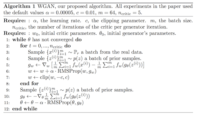
Algorithm for the Wasserstein Generative Adversarial Networks.
Taken from: Wasserstein GAN.
The differences in implementation for the WGAN are as follows:
- Use a linear activation function in the output layer of the critic model (instead of sigmoid).
- Use -1 labels for real images and 1 labels for fake images (instead of 1 and 0).
- Use Wasserstein loss to train the critic and generator models.
- Constrain critic model weights to a limited range after each mini batch update (e.g. [-0.01,0.01]).
- Update the critic model more times than the generator each iteration (e.g. 5).
- Use the RMSProp version of gradient descent with a small learning rate and no momentum (e.g. 0.00005).
Using the standard DCGAN model as a starting point, let’s take a look at each of these implementation details in turn.
Want to Develop GANs from Scratch?
Take my free 7-day email crash course now (with sample code).
Click to sign-up and also get a free PDF Ebook version of the course.
1. Linear Activation in Critic Output Layer
The DCGAN uses the sigmoid activation function in the output layer of the discriminator to predict the likelihood of a given image being real.
In the WGAN, the critic model requires a linear activation to predict the score of “realness” for a given image.
This can be achieved by setting the ‘activation‘ argument to ‘linear‘ in the output layer of the critic model.
|
1 2 3 |
# define output layer of the critic model ... model.add(Dense(1, activation='linear')) |
The linear activation is the default activation for a layer, so we can, in fact, leave the activation unspecified to achieve the same result.
|
1 2 3 |
# define output layer of the critic model ... model.add(Dense(1)) |
2. Class Labels for Real and Fake Images
The DCGAN uses the class 0 for fake images and class 1 for real images, and these class labels are used to train the GAN.
In the DCGAN, these are precise labels that the discriminator is expected to achieve. The WGAN does not have precise labels for the critic. Instead, it encourages the critic to output scores that are different for real and fake images.
This is achieved via the Wasserstein function that cleverly makes use of positive and negative class labels.
The WGAN can be implemented where -1 class labels are used for real images and +1 class labels are used for fake or generated images.
This can be achieved using the ones() NumPy function.
For example:
|
1 2 3 4 5 6 |
... # generate class labels, -1 for 'real' y = -ones((n_samples, 1)) ... # create class labels with 1.0 for 'fake' y = ones((n_samples, 1)) |
3. Wasserstein Loss Function
The DCGAN trains the discriminator as a binary classification model to predict the probability that a given image is real.
To train this model, the discriminator is optimized using the binary cross entropy loss function. The same loss function is used to update the generator model.
The primary contribution of the WGAN model is the use of a new loss function that encourages the discriminator to predict a score of how real or fake a given input looks. This transforms the role of the discriminator from a classifier into a critic for scoring the realness or fakeness of images, where the difference between the scores is as large as possible.
We can implement the Wasserstein loss as a custom function in Keras that calculates the average score for real or fake images.
The score is maximizing for real examples and minimizing for fake examples. Given that stochastic gradient descent is a minimization algorithm, we can multiply the class label by the mean score (e.g. -1 for real and 1 for fake which as no effect), which ensures that the loss for real and fake images is minimizing to the network.
An efficient implementation of this loss function for Keras is listed below.
|
1 2 3 4 5 |
from keras import backend # implementation of wasserstein loss def wasserstein_loss(y_true, y_pred): return backend.mean(y_true * y_pred) |
This loss function can be used to train a Keras model by specifying the function name when compiling the model.
For example:
|
1 2 3 |
... # compile the model model.compile(loss=wasserstein_loss, ...) |
4. Critic Weight Clipping
The DCGAN does not use any gradient clipping, although the WGAN requires gradient clipping for the critic model.
We can implement weight clipping as a Keras constraint.
This is a class that must extend the Constraint class and define an implementation of the __call__() function for applying the operation and the get_config() function for returning any configuration.
We can also define an __init__() function to set the configuration, in this case, the symmetrical size of the bounding box for the weight hypercube, e.g. 0.01.
The ClipConstraint class is defined below.
|
1 2 3 4 5 6 7 8 9 10 11 12 13 |
# clip model weights to a given hypercube class ClipConstraint(Constraint): # set clip value when initialized def __init__(self, clip_value): self.clip_value = clip_value # clip model weights to hypercube def __call__(self, weights): return backend.clip(weights, -self.clip_value, self.clip_value) # get the config def get_config(self): return {'clip_value': self.clip_value} |
To use the constraint, the class can be constructed, then used in a layer by setting the kernel_constraint argument; for example:
|
1 2 3 4 5 6 |
... # define the constraint const = ClipConstraint(0.01) ... # use the constraint in a layer model.add(Conv2D(..., kernel_constraint=const)) |
The constraint is only required when updating the critic model.
5. Update Critic More Than Generator
In the DCGAN, the generator and the discriminator model must be updated in equal amounts.
Specifically, the discriminator is updated with a half batch of real and a half batch of fake samples each iteration, whereas the generator is updated with a single batch of generated samples.
For example:
|
1 2 3 4 5 6 7 8 9 10 11 12 13 14 15 16 17 18 19 20 21 22 23 |
... # main gan training loop for i in range(n_steps): # update the discriminator # get randomly selected 'real' samples X_real, y_real = generate_real_samples(dataset, half_batch) # update critic model weights c_loss1 = c_model.train_on_batch(X_real, y_real) # generate 'fake' examples X_fake, y_fake = generate_fake_samples(g_model, latent_dim, half_batch) # update critic model weights c_loss2 = c_model.train_on_batch(X_fake, y_fake) # update generator # prepare points in latent space as input for the generator X_gan = generate_latent_points(latent_dim, n_batch) # create inverted labels for the fake samples y_gan = ones((n_batch, 1)) # update the generator via the critic's error g_loss = gan_model.train_on_batch(X_gan, y_gan) |
In the WGAN model, the critic model must be updated more than the generator model.
Specifically, a new hyperparameter is defined to control the number of times that the critic is updated for each update to the generator model, called n_critic, and is set to 5.
This can be implemented as a new loop within the main GAN update loop; for example:
|
1 2 3 4 5 6 7 8 9 10 11 12 13 14 15 16 17 18 19 20 21 22 23 |
... # main gan training loop for i in range(n_steps): # update the critic for _ in range(n_critic): # get randomly selected 'real' samples X_real, y_real = generate_real_samples(dataset, half_batch) # update critic model weights c_loss1 = c_model.train_on_batch(X_real, y_real) # generate 'fake' examples X_fake, y_fake = generate_fake_samples(g_model, latent_dim, half_batch) # update critic model weights c_loss2 = c_model.train_on_batch(X_fake, y_fake) # update generator # prepare points in latent space as input for the generator X_gan = generate_latent_points(latent_dim, n_batch) # create inverted labels for the fake samples y_gan = ones((n_batch, 1)) # update the generator via the critic's error g_loss = gan_model.train_on_batch(X_gan, y_gan) |
6. Use RMSProp Stochastic Gradient Descent
The DCGAN uses the Adam version of stochastic gradient descent with a small learning rate and modest momentum.
The WGAN recommends the use of RMSProp instead, with a small learning rate of 0.00005.
This can be implemented in Keras when the model is compiled. For example:
|
1 2 3 4 |
... # compile model opt = RMSprop(lr=0.00005) model.compile(loss=wasserstein_loss, optimizer=opt) |
How to Train a Wasserstein GAN Model
Now that we know the specific implementation details for the WGAN, we can implement the model for image generation.
In this section, we will develop a WGAN to generate a single handwritten digit (‘7’) from the MNIST dataset. This is a good test problem for the WGAN as it is a small dataset requiring a modest mode that is quick to train.
The first step is to define the models.
The critic model takes as input one 28×28 grayscale image and outputs a score for the realness or fakeness of the image. It is implemented as a modest convolutional neural network using best practices for DCGAN design such as using the LeakyReLU activation function with a slope of 0.2, batch normalization, and using a 2×2 stride to downsample.
The critic model makes use of the new ClipConstraint weight constraint to clip model weights after mini-batch updates and is optimized using the custom wasserstein_loss() function, the RMSProp version of stochastic gradient descent with a learning rate of 0.00005.
The define_critic() function below implements this, defining and compiling the critic model and returning it. The input shape of the image is parameterized as a default function argument to make it clear.
|
1 2 3 4 5 6 7 8 9 10 11 12 13 14 15 16 17 18 19 20 21 22 23 |
# define the standalone critic model def define_critic(in_shape=(28,28,1)): # weight initialization init = RandomNormal(stddev=0.02) # weight constraint const = ClipConstraint(0.01) # define model model = Sequential() # downsample to 14x14 model.add(Conv2D(64, (4,4), strides=(2,2), padding='same', kernel_initializer=init, kernel_constraint=const, input_shape=in_shape)) model.add(BatchNormalization()) model.add(LeakyReLU(alpha=0.2)) # downsample to 7x7 model.add(Conv2D(64, (4,4), strides=(2,2), padding='same', kernel_initializer=init, kernel_constraint=const)) model.add(BatchNormalization()) model.add(LeakyReLU(alpha=0.2)) # scoring, linear activation model.add(Flatten()) model.add(Dense(1)) # compile model opt = RMSprop(lr=0.00005) model.compile(loss=wasserstein_loss, optimizer=opt) return model |
The generator model takes as input a point in the latent space and outputs a single 28×28 grayscale image.
This is achieved by using a fully connected layer to interpret the point in the latent space and provide sufficient activations that can be reshaped into many copies (in this case, 128) of a low-resolution version of the output image (e.g. 7×7). This is then upsampled two times, doubling the size and quadrupling the area of the activations each time using transpose convolutional layers.
The model uses best practices such as the LeakyReLU activation, a kernel size that is a factor of the stride size, and a hyperbolic tangent (tanh) activation function in the output layer.
The define_generator() function below defines the generator model but intentionally does not compile it as it is not trained directly, then returns the model. The size of the latent space is parameterized as a function argument.
|
1 2 3 4 5 6 7 8 9 10 11 12 13 14 15 16 17 18 19 20 21 22 |
# define the standalone generator model def define_generator(latent_dim): # weight initialization init = RandomNormal(stddev=0.02) # define model model = Sequential() # foundation for 7x7 image n_nodes = 128 * 7 * 7 model.add(Dense(n_nodes, kernel_initializer=init, input_dim=latent_dim)) model.add(LeakyReLU(alpha=0.2)) model.add(Reshape((7, 7, 128))) # upsample to 14x14 model.add(Conv2DTranspose(128, (4,4), strides=(2,2), padding='same', kernel_initializer=init)) model.add(BatchNormalization()) model.add(LeakyReLU(alpha=0.2)) # upsample to 28x28 model.add(Conv2DTranspose(128, (4,4), strides=(2,2), padding='same', kernel_initializer=init)) model.add(BatchNormalization()) model.add(LeakyReLU(alpha=0.2)) # output 28x28x1 model.add(Conv2D(1, (7,7), activation='tanh', padding='same', kernel_initializer=init)) return model |
Next, a GAN model can be defined that combines both the generator model and the critic model into one larger model.
This larger model will be used to train the model weights in the generator, using the output and error calculated by the critic model. The critic model is trained separately, and as such, the model weights are marked as not trainable in this larger GAN model to ensure that only the weights of the generator model are updated. This change to the trainability of the critic weights only has an effect when training the combined GAN model, not when training the critic standalone.
This larger GAN model takes as input a point in the latent space, uses the generator model to generate an image, which is fed as input to the critic model, then output scored as real or fake. The model is fit using RMSProp with the custom wasserstein_loss() function.
The define_gan() function below implements this, taking the already defined generator and critic models as input.
|
1 2 3 4 5 6 7 8 9 10 11 12 13 14 15 16 |
# define the combined generator and critic model, for updating the generator def define_gan(generator, critic): # make weights in the critic not trainable for layer in critic.layers: if not isinstance(layer, BatchNormalization): layer.trainable = False # connect them model = Sequential() # add generator model.add(generator) # add the critic model.add(critic) # compile model opt = RMSprop(lr=0.00005) model.compile(loss=wasserstein_loss, optimizer=opt) return model |
Now that we have defined the GAN model, we need to train it. But, before we can train the model, we require input data.
The first step is to load and scale the MNIST dataset. The whole dataset is loaded via a call to the load_data() Keras function, then a subset of the images is selected (about 5,000) that belongs to class 7, e.g. are a handwritten depiction of the number seven. Then the pixel values must be scaled to the range [-1,1] to match the output of the generator model.
The load_real_samples() function below implements this, returning the loaded and scaled subset of the MNIST training dataset ready for modeling.
|
1 2 3 4 5 6 7 8 9 10 11 12 13 14 |
# load images def load_real_samples(): # load dataset (trainX, trainy), (_, _) = load_data() # select all of the examples for a given class selected_ix = trainy == 7 X = trainX[selected_ix] # expand to 3d, e.g. add channels X = expand_dims(X, axis=-1) # convert from ints to floats X = X.astype('float32') # scale from [0,255] to [-1,1] X = (X - 127.5) / 127.5 return X |
We will require one batch (or a half) batch of real images from the dataset each update to the GAN model. A simple way to achieve this is to select a random sample of images from the dataset each time.
The generate_real_samples() function below implements this, taking the prepared dataset as an argument, selecting and returning a random sample of images and their corresponding label for the critic, specifically target=-1 indicating that they are real images.
|
1 2 3 4 5 6 7 8 9 |
# select real samples def generate_real_samples(dataset, n_samples): # choose random instances ix = randint(0, dataset.shape[0], n_samples) # select images X = dataset[ix] # generate class labels, -1 for 'real' y = -ones((n_samples, 1)) return X, y |
Next, we need inputs for the generator model. These are random points from the latent space, specifically Gaussian distributed random variables.
The generate_latent_points() function implements this, taking the size of the latent space as an argument and the number of points required, and returning them as a batch of input samples for the generator model.
|
1 2 3 4 5 6 7 |
# generate points in latent space as input for the generator def generate_latent_points(latent_dim, n_samples): # generate points in the latent space x_input = randn(latent_dim * n_samples) # reshape into a batch of inputs for the network x_input = x_input.reshape(n_samples, latent_dim) return x_input |
Next, we need to use the points in the latent space as input to the generator in order to generate new images.
The generate_fake_samples() function below implements this, taking the generator model and size of the latent space as arguments, then generating points in the latent space and using them as input to the generator model.
The function returns the generated images and their corresponding label for the critic model, specifically target=1 to indicate they are fake or generated.
|
1 2 3 4 5 6 7 8 9 |
# use the generator to generate n fake examples, with class labels def generate_fake_samples(generator, latent_dim, n_samples): # generate points in latent space x_input = generate_latent_points(latent_dim, n_samples) # predict outputs X = generator.predict(x_input) # create class labels with 1.0 for 'fake' y = ones((n_samples, 1)) return X, y |
We need to record the performance of the model. Perhaps the most reliable way to evaluate the performance of a GAN is to use the generator to generate images, and then review and subjectively evaluate them.
The summarize_performance() function below takes the generator model at a given point during training and uses it to generate 100 images in a 10×10 grid, that are then plotted and saved to file. The model is also saved to file at this time, in case we would like to use it later to generate more images.
|
1 2 3 4 5 6 7 8 9 10 11 12 13 14 15 16 17 18 19 20 21 22 |
# generate samples and save as a plot and save the model def summarize_performance(step, g_model, latent_dim, n_samples=100): # prepare fake examples X, _ = generate_fake_samples(g_model, latent_dim, n_samples) # scale from [-1,1] to [0,1] X = (X + 1) / 2.0 # plot images for i in range(10 * 10): # define subplot pyplot.subplot(10, 10, 1 + i) # turn off axis pyplot.axis('off') # plot raw pixel data pyplot.imshow(X[i, :, :, 0], cmap='gray_r') # save plot to file filename1 = 'generated_plot_%04d.png' % (step+1) pyplot.savefig(filename1) pyplot.close() # save the generator model filename2 = 'model_%04d.h5' % (step+1) g_model.save(filename2) print('>Saved: %s and %s' % (filename1, filename2)) |
In addition to image quality, it is a good idea to keep track of the loss and accuracy of the model over time.
The loss for the critic for real and fake samples can be tracked for each model update, as can the loss for the generator for each update. These can then be used to create line plots of loss at the end of the training run. The plot_history() function below implements this and saves the results to file.
|
1 2 3 4 5 6 7 8 9 |
# create a line plot of loss for the gan and save to file def plot_history(d1_hist, d2_hist, g_hist): # plot history pyplot.plot(d1_hist, label='crit_real') pyplot.plot(d2_hist, label='crit_fake') pyplot.plot(g_hist, label='gen') pyplot.legend() pyplot.savefig('plot_line_plot_loss.png') pyplot.close() |
We are now ready to fit the GAN model.
The model is fit for 10 training epochs, which is arbitrary, as the model begins generating plausible number-7 digits after perhaps the first few epochs. A batch size of 64 samples is used, and each training epoch involves 6,265/64, or about 97, batches of real and fake samples and updates to the model. The model is therefore trained for 10 epochs of 97 batches, or 970 iterations.
First, the critic model is updated for a half batch of real samples, then a half batch of fake samples, together forming one batch of weight updates. This is then repeated n_critic (5) times as required by the WGAN algorithm.
The generator is then updated via the composite GAN model. Importantly, the target label is set to -1 or real for the generated samples. This has the effect of updating the generator toward getting better at generating real samples on the next batch.
The train() function below implements this, taking the defined models, dataset, and size of the latent dimension as arguments and parameterizing the number of epochs and batch size with default arguments. The generator model is saved at the end of training.
The performance of the critic and generator models is reported each iteration. Sample images are generated and saved every epoch, and line plots of model performance are created and saved at the end of the run.
|
1 2 3 4 5 6 7 8 9 10 11 12 13 14 15 16 17 18 19 20 21 22 23 24 25 26 27 28 29 30 31 32 33 34 35 36 37 38 39 40 41 42 |
# train the generator and critic def train(g_model, c_model, gan_model, dataset, latent_dim, n_epochs=10, n_batch=64, n_critic=5): # calculate the number of batches per training epoch bat_per_epo = int(dataset.shape[0] / n_batch) # calculate the number of training iterations n_steps = bat_per_epo * n_epochs # calculate the size of half a batch of samples half_batch = int(n_batch / 2) # lists for keeping track of loss c1_hist, c2_hist, g_hist = list(), list(), list() # manually enumerate epochs for i in range(n_steps): # update the critic more than the generator c1_tmp, c2_tmp = list(), list() for _ in range(n_critic): # get randomly selected 'real' samples X_real, y_real = generate_real_samples(dataset, half_batch) # update critic model weights c_loss1 = c_model.train_on_batch(X_real, y_real) c1_tmp.append(c_loss1) # generate 'fake' examples X_fake, y_fake = generate_fake_samples(g_model, latent_dim, half_batch) # update critic model weights c_loss2 = c_model.train_on_batch(X_fake, y_fake) c2_tmp.append(c_loss2) # store critic loss c1_hist.append(mean(c1_tmp)) c2_hist.append(mean(c2_tmp)) # prepare points in latent space as input for the generator X_gan = generate_latent_points(latent_dim, n_batch) # create inverted labels for the fake samples y_gan = -ones((n_batch, 1)) # update the generator via the critic's error g_loss = gan_model.train_on_batch(X_gan, y_gan) g_hist.append(g_loss) # summarize loss on this batch print('>%d, c1=%.3f, c2=%.3f g=%.3f' % (i+1, c1_hist[-1], c2_hist[-1], g_loss)) # evaluate the model performance every 'epoch' if (i+1) % bat_per_epo == 0: summarize_performance(i, g_model, latent_dim) # line plots of loss plot_history(c1_hist, c2_hist, g_hist) |
Now that all of the functions have been defined, we can create the models, load the dataset, and begin the training process.
|
1 2 3 4 5 6 7 8 9 10 11 12 13 |
# size of the latent space latent_dim = 50 # create the critic critic = define_critic() # create the generator generator = define_generator(latent_dim) # create the gan gan_model = define_gan(generator, critic) # load image data dataset = load_real_samples() print(dataset.shape) # train model train(generator, critic, gan_model, dataset, latent_dim) |
Tying all of this together, the complete example is listed below.
|
1 2 3 4 5 6 7 8 9 10 11 12 13 14 15 16 17 18 19 20 21 22 23 24 25 26 27 28 29 30 31 32 33 34 35 36 37 38 39 40 41 42 43 44 45 46 47 48 49 50 51 52 53 54 55 56 57 58 59 60 61 62 63 64 65 66 67 68 69 70 71 72 73 74 75 76 77 78 79 80 81 82 83 84 85 86 87 88 89 90 91 92 93 94 95 96 97 98 99 100 101 102 103 104 105 106 107 108 109 110 111 112 113 114 115 116 117 118 119 120 121 122 123 124 125 126 127 128 129 130 131 132 133 134 135 136 137 138 139 140 141 142 143 144 145 146 147 148 149 150 151 152 153 154 155 156 157 158 159 160 161 162 163 164 165 166 167 168 169 170 171 172 173 174 175 176 177 178 179 180 181 182 183 184 185 186 187 188 189 190 191 192 193 194 195 196 197 198 199 200 201 202 203 204 205 206 207 208 209 210 211 212 213 214 215 216 217 218 219 220 221 222 223 224 225 226 227 228 229 230 231 232 233 234 235 |
# example of a wgan for generating handwritten digits from numpy import expand_dims from numpy import mean from numpy import ones from numpy.random import randn from numpy.random import randint from keras.datasets.mnist import load_data from keras import backend from keras.optimizers import RMSprop from keras.models import Sequential from keras.layers import Dense from keras.layers import Reshape from keras.layers import Flatten from keras.layers import Conv2D from keras.layers import Conv2DTranspose from keras.layers import LeakyReLU from keras.layers import BatchNormalization from keras.initializers import RandomNormal from keras.constraints import Constraint from matplotlib import pyplot # clip model weights to a given hypercube class ClipConstraint(Constraint): # set clip value when initialized def __init__(self, clip_value): self.clip_value = clip_value # clip model weights to hypercube def __call__(self, weights): return backend.clip(weights, -self.clip_value, self.clip_value) # get the config def get_config(self): return {'clip_value': self.clip_value} # calculate wasserstein loss def wasserstein_loss(y_true, y_pred): return backend.mean(y_true * y_pred) # define the standalone critic model def define_critic(in_shape=(28,28,1)): # weight initialization init = RandomNormal(stddev=0.02) # weight constraint const = ClipConstraint(0.01) # define model model = Sequential() # downsample to 14x14 model.add(Conv2D(64, (4,4), strides=(2,2), padding='same', kernel_initializer=init, kernel_constraint=const, input_shape=in_shape)) model.add(BatchNormalization()) model.add(LeakyReLU(alpha=0.2)) # downsample to 7x7 model.add(Conv2D(64, (4,4), strides=(2,2), padding='same', kernel_initializer=init, kernel_constraint=const)) model.add(BatchNormalization()) model.add(LeakyReLU(alpha=0.2)) # scoring, linear activation model.add(Flatten()) model.add(Dense(1)) # compile model opt = RMSprop(lr=0.00005) model.compile(loss=wasserstein_loss, optimizer=opt) return model # define the standalone generator model def define_generator(latent_dim): # weight initialization init = RandomNormal(stddev=0.02) # define model model = Sequential() # foundation for 7x7 image n_nodes = 128 * 7 * 7 model.add(Dense(n_nodes, kernel_initializer=init, input_dim=latent_dim)) model.add(LeakyReLU(alpha=0.2)) model.add(Reshape((7, 7, 128))) # upsample to 14x14 model.add(Conv2DTranspose(128, (4,4), strides=(2,2), padding='same', kernel_initializer=init)) model.add(BatchNormalization()) model.add(LeakyReLU(alpha=0.2)) # upsample to 28x28 model.add(Conv2DTranspose(128, (4,4), strides=(2,2), padding='same', kernel_initializer=init)) model.add(BatchNormalization()) model.add(LeakyReLU(alpha=0.2)) # output 28x28x1 model.add(Conv2D(1, (7,7), activation='tanh', padding='same', kernel_initializer=init)) return model # define the combined generator and critic model, for updating the generator def define_gan(generator, critic): # make weights in the critic not trainable for layer in critic.layers: if not isinstance(layer, BatchNormalization): layer.trainable = False # connect them model = Sequential() # add generator model.add(generator) # add the critic model.add(critic) # compile model opt = RMSprop(lr=0.00005) model.compile(loss=wasserstein_loss, optimizer=opt) return model # load images def load_real_samples(): # load dataset (trainX, trainy), (_, _) = load_data() # select all of the examples for a given class selected_ix = trainy == 7 X = trainX[selected_ix] # expand to 3d, e.g. add channels X = expand_dims(X, axis=-1) # convert from ints to floats X = X.astype('float32') # scale from [0,255] to [-1,1] X = (X - 127.5) / 127.5 return X # select real samples def generate_real_samples(dataset, n_samples): # choose random instances ix = randint(0, dataset.shape[0], n_samples) # select images X = dataset[ix] # generate class labels, -1 for 'real' y = -ones((n_samples, 1)) return X, y # generate points in latent space as input for the generator def generate_latent_points(latent_dim, n_samples): # generate points in the latent space x_input = randn(latent_dim * n_samples) # reshape into a batch of inputs for the network x_input = x_input.reshape(n_samples, latent_dim) return x_input # use the generator to generate n fake examples, with class labels def generate_fake_samples(generator, latent_dim, n_samples): # generate points in latent space x_input = generate_latent_points(latent_dim, n_samples) # predict outputs X = generator.predict(x_input) # create class labels with 1.0 for 'fake' y = ones((n_samples, 1)) return X, y # generate samples and save as a plot and save the model def summarize_performance(step, g_model, latent_dim, n_samples=100): # prepare fake examples X, _ = generate_fake_samples(g_model, latent_dim, n_samples) # scale from [-1,1] to [0,1] X = (X + 1) / 2.0 # plot images for i in range(10 * 10): # define subplot pyplot.subplot(10, 10, 1 + i) # turn off axis pyplot.axis('off') # plot raw pixel data pyplot.imshow(X[i, :, :, 0], cmap='gray_r') # save plot to file filename1 = 'generated_plot_%04d.png' % (step+1) pyplot.savefig(filename1) pyplot.close() # save the generator model filename2 = 'model_%04d.h5' % (step+1) g_model.save(filename2) print('>Saved: %s and %s' % (filename1, filename2)) # create a line plot of loss for the gan and save to file def plot_history(d1_hist, d2_hist, g_hist): # plot history pyplot.plot(d1_hist, label='crit_real') pyplot.plot(d2_hist, label='crit_fake') pyplot.plot(g_hist, label='gen') pyplot.legend() pyplot.savefig('plot_line_plot_loss.png') pyplot.close() # train the generator and critic def train(g_model, c_model, gan_model, dataset, latent_dim, n_epochs=10, n_batch=64, n_critic=5): # calculate the number of batches per training epoch bat_per_epo = int(dataset.shape[0] / n_batch) # calculate the number of training iterations n_steps = bat_per_epo * n_epochs # calculate the size of half a batch of samples half_batch = int(n_batch / 2) # lists for keeping track of loss c1_hist, c2_hist, g_hist = list(), list(), list() # manually enumerate epochs for i in range(n_steps): # update the critic more than the generator c1_tmp, c2_tmp = list(), list() for _ in range(n_critic): # get randomly selected 'real' samples X_real, y_real = generate_real_samples(dataset, half_batch) # update critic model weights c_loss1 = c_model.train_on_batch(X_real, y_real) c1_tmp.append(c_loss1) # generate 'fake' examples X_fake, y_fake = generate_fake_samples(g_model, latent_dim, half_batch) # update critic model weights c_loss2 = c_model.train_on_batch(X_fake, y_fake) c2_tmp.append(c_loss2) # store critic loss c1_hist.append(mean(c1_tmp)) c2_hist.append(mean(c2_tmp)) # prepare points in latent space as input for the generator X_gan = generate_latent_points(latent_dim, n_batch) # create inverted labels for the fake samples y_gan = -ones((n_batch, 1)) # update the generator via the critic's error g_loss = gan_model.train_on_batch(X_gan, y_gan) g_hist.append(g_loss) # summarize loss on this batch print('>%d, c1=%.3f, c2=%.3f g=%.3f' % (i+1, c1_hist[-1], c2_hist[-1], g_loss)) # evaluate the model performance every 'epoch' if (i+1) % bat_per_epo == 0: summarize_performance(i, g_model, latent_dim) # line plots of loss plot_history(c1_hist, c2_hist, g_hist) # size of the latent space latent_dim = 50 # create the critic critic = define_critic() # create the generator generator = define_generator(latent_dim) # create the gan gan_model = define_gan(generator, critic) # load image data dataset = load_real_samples() print(dataset.shape) # train model train(generator, critic, gan_model, dataset, latent_dim) |
Running the example is quick, taking approximately 10 minutes on modern hardware without a GPU.
Note: Your results may vary given the stochastic nature of the algorithm or evaluation procedure, or differences in numerical precision. Consider running the example a few times and compare the average outcome.
First, the loss of the critic and generator models is reported to the console each iteration of the training loop. Specifically, c1 is the loss of the critic on real examples, c2 is the loss of the critic in generated samples, and g is the loss of the generator trained via the critic.
The c1 scores are inverted as part of the loss function; this means if they are reported as negative, then they are really positive, and if they are reported as positive, they are really negative. The sign of the c2 scores is unchanged.
Recall that the Wasserstein loss seeks scores for real and fake that are more different during training. We can see this towards the end of the run, such as the final epoch where the c1 loss for real examples is 5.338 (really -5.338) and the c2 loss for fake examples is -14.260, and this separation of about 10 units is consistent at least for the prior few iterations.
We can also see that in this case, the model is scoring the loss of the generator at around 20. Again, recall that we update the generator via the critic model and treat the generated examples as real with the target of -1, therefore the score can be interpreted as a value around -20, close to the loss for fake samples.
|
1 2 3 4 5 6 7 8 9 10 11 |
... >961, c1=5.110, c2=-15.388 g=19.579 >962, c1=6.116, c2=-15.222 g=20.054 >963, c1=4.982, c2=-15.192 g=21.048 >964, c1=4.238, c2=-14.689 g=23.911 >965, c1=5.585, c2=-14.126 g=19.578 >966, c1=4.807, c2=-14.755 g=20.034 >967, c1=6.307, c2=-16.538 g=19.572 >968, c1=4.298, c2=-14.178 g=17.956 >969, c1=4.283, c2=-13.398 g=17.326 >970, c1=5.338, c2=-14.260 g=19.927 |
Line plots for loss are created and saved at the end of the run.
The plot shows the loss for the critic on real samples (blue), the loss for the critic on fake samples (orange), and the loss for the critic when updating the generator with fake samples (green).
There is one important factor when reviewing learning curves for the WGAN and that is the trend.
The benefit of the WGAN is that the loss correlates with generated image quality. Lower loss means better quality images, for a stable training process.
In this case, lower loss specifically refers to lower Wasserstein loss for generated images as reported by the critic (orange line). This sign of this loss is not inverted by the target label (e.g. the target label is +1.0), therefore, a well-performing WGAN should show this line trending down as the image quality of the generated model is increased.

Line Plots of Loss and Accuracy for a Wasserstein Generative Adversarial Network
In this case, more training seems to result in better quality generated images, with a major hurdle occurring around epoch 200-300 after which quality remains pretty good for the model.
Before and around this hurdle, image quality is poor; for example:
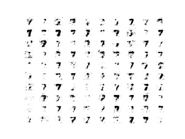
Sample of 100 Generated Images of a Handwritten Number 7 at Epoch 97 from a Wasserstein GAN.
After this epoch, the WGAN continues to generate plausible handwritten digits.
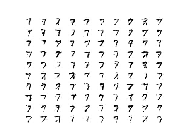
Sample of 100 Generated Images of a Handwritten Number 7 at Epoch 970 from a Wasserstein GAN.
Further Reading
This section provides more resources on the topic if you are looking to go deeper.
Papers
- Wasserstein GAN, 2017.
- Improved Training of Wasserstein GANs, 2017.
API
- Keras Datasets API.
- Keras Sequential Model API
- Keras Convolutional Layers API
- How can I “freeze” Keras layers?
- MatplotLib API
- NumPy Random sampling (numpy.random) API
- NumPy Array manipulation routines
Articles
- WassersteinGAN, GitHub.
- Wasserstein Generative Adversarial Networks (WGANS) Project, GitHub.
- Keras-GAN: Keras implementations of Generative Adversarial Networks, GitHub.
- Improved WGAN, keras-contrib Project, GitHub.
Summary
In this tutorial, you discovered how to implement the Wasserstein generative adversarial network from scratch.
Specifically, you learned:
- The differences between the standard deep convolutional GAN and the new Wasserstein GAN.
- How to implement the specific details of the Wasserstein GAN from scratch.
- How to develop a WGAN for image generation and interpret the dynamic behavior of the model.
Do you have any questions?
Ask your questions in the comments below and I will do my best to answer.
Develop Generative Adversarial Networks Today!
Develop Your GAN Models in Minutes
...with just a few lines of python codeDiscover how in my new Ebook:
Generative Adversarial Networks with Python
It provides self-study tutorials and end-to-end projects on:
DCGAN, conditional GANs, image translation, Pix2Pix, CycleGAN
and much more...


 in Keras")


Thank for your great tutorial
I am curious about 2 things:
1. What is exactly clipping weight does? (I read the source code of Keras for clip_by_value() function but I can’t figure out what exactly it does)
2. According to your previous article, I knew that Critic’s outcome is just a real number for optimizing the generator, as long as critic(fake) > critic(real). The critic is Wasserstein distance. Therefore, can Wasserstein loss use in common CNN replacing CNN loss function like MSE, PSNR? say, I am training a deblurring CNN using Wasserstein loss, if I minimize this loss value, then my CNN will converge? Am I correct?
Thank for reading my question
Good questions.
The weight clipping ensure weight values (model parameters) stay within a pre-defined bounds.
You can use MSE instead, but it is different. In fact, this is called a least-squares GAN and does not convergence, but does very well.
Thank for your response!
In my question 1, I still confuse about “stay within pre-defined bounds”. In my question 2, There is a misunderstanding.
Question 1: Assume I have weights like this W = [0.3 -2.5, 4.5, 0.05, -0.02] then what is the result of clip(W, (-0.1, 0.1)) ?
Question 2: I know least-squares GAN, my question is: “how to adopt Wasserstein loss metric as loss function in NORMAL architecture CNN (not GAN architecture)?”. I did search on the internet to find the answer but there is no study adopting this Wasserstein Distance as their loss function in normal CNN. I didn’t figure out the reason why they didn’t use it.
I am so sorry for my bad English
Hope you get what I mean.
Thank you
Good questions.
The clipping is defined as:
– If a weight is less than -0.01, it is set to -0.01.
– If a weight is more than 0.01, it is set to 0.01.
I’m not sure it is an appropriate loss function for a normal image classification task. i.e. you cannot.
Thank you very much, Sir
You’re welcome.
Great article!
I trained the GAN on all 9 digits and the results are wild. Lots of digits that look halfway between one digit and another… my model loves generating 0&8 hybrids. Have a few ideas for limiting this effect such as : using a bigger latent space, feeding the class as input into the network, using a bigger conv model, maybe adding a fc layer that appends to the output of the discriminator that my model can use as a class predictor(??) and obviously training longer.
Well done James!
So i implemented your model just as you provided it, but my loss functions look entirely different. Crit_real and crit_fake drop all the way down to -150 after 400 epochs while gen goes to 150 after 400 epochs.
Up to that point the resulting images look good, but afterwards they just turn all black.
Can you give an explanation why this would happen?
You changed the loss function and got bad results. Sorry, I don’t know why other than you changed the loss function.
Perhaps try the code as listed first?
I am implementing the same model in my own framework, and I am having similar issues : like black images. I narrowed the problem down to the fact that the way we initializing things arbitrarily like the weights of the convolution/Conv2dTranspose filters. It is done differently in different frameworks, so the same hyperparameters will not work for someone running different frameworks.
Hi Hidden Machine…Weight initialization is a critical aspect of training neural networks, especially in Generative Adversarial Networks (GANs) like WGANs. Different frameworks might have different default initialization methods, leading to variations in training performance. Here’s a step-by-step guide to initializing weights properly for a WGAN implementation in your custom framework.
### Weight Initialization for WGAN
To achieve consistent results across different frameworks, you can use specific weight initialization methods like Xavier (Glorot) initialization or He initialization. Here’s how you can implement Xavier initialization in a WGAN from scratch.
#### Step-by-Step Implementation
1. **Define Xavier Initialization Function:**
pythonimport numpy as np
def xavier_init(size):
in_dim = size[0]
xavier_stddev = 1. / np.sqrt(in_dim / 2.)
return np.random.normal(0, xavier_stddev, size=size)
2. **Apply Xavier Initialization to Model Weights:**
When defining your model layers (e.g., convolutional layers), you can apply the Xavier initialization function to initialize the weights.
pythonimport torch
import torch.nn as nn
def weights_init_xavier(m):
classname = m.__class__.__name__
if classname.find('Conv') != -1 or classname.find('Linear') != -1:
fan_in, fan_out = nn.init._calculate_fan_in_and_fan_out(m.weight.data)
std = np.sqrt(2.0 / (fan_in + fan_out))
nn.init.normal_(m.weight.data, 0.0, std)
if m.bias is not None:
m.bias.data.fill_(0)
class Generator(nn.Module):
def __init__(self, z_dim):
super(Generator, self).__init__()
self.main = nn.Sequential(
# Define your layers here
)
def forward(self, x):
return self.main(x)
class Discriminator(nn.Module):
def __init__(self):
super(Discriminator, self).__init__()
self.main = nn.Sequential(
# Define your layers here
)
def forward(self, x):
return self.main(x)
z_dim = 100
G = Generator(z_dim)
D = Discriminator()
# Apply Xavier initialization
G.apply(weights_init_xavier)
D.apply(weights_init_xavier)
3. **Implement the WGAN Training Loop:**
Make sure you follow the WGAN training procedure, including the use of the Wasserstein loss and gradient penalty.
pythonimport torch.optim as optim
def gradient_penalty(D, real_data, fake_data):
alpha = torch.rand(real_data.size(0), 1, 1, 1).to(real_data.device)
interpolates = alpha * real_data + ((1 - alpha) * fake_data)
interpolates = interpolates.requires_grad_(True)
d_interpolates = D(interpolates)
fake = torch.ones(d_interpolates.size()).to(real_data.device)
gradients = torch.autograd.grad(outputs=d_interpolates, inputs=interpolates,
grad_outputs=fake, create_graph=True, retain_graph=True, only_inputs=True)[0]
gradients = gradients.view(gradients.size(0), -1)
gradient_penalty = ((gradients.norm(2, dim=1) - 1) ** 2).mean()
return gradient_penalty
lr = 0.0002
betas = (0.5, 0.999)
n_critic = 5
lambda_gp = 10
optimizer_D = optim.Adam(D.parameters(), lr=lr, betas=betas)
optimizer_G = optim.Adam(G.parameters(), lr=lr, betas=betas)
for epoch in range(num_epochs):
for i, (real_images, _) in enumerate(dataloader):
real_images = real_images.to(device)
# Train Discriminator
for _ in range(n_critic):
noise = torch.randn(batch_size, z_dim, 1, 1).to(device)
fake_images = G(noise)
real_validity = D(real_images)
fake_validity = D(fake_images)
gp = gradient_penalty(D, real_images.data, fake_images.data)
d_loss = -torch.mean(real_validity) + torch.mean(fake_validity) + lambda_gp * gp
optimizer_D.zero_grad()
d_loss.backward()
optimizer_D.step()
# Train Generator
noise = torch.randn(batch_size, z_dim, 1, 1).to(device)
fake_images = G(noise)
fake_validity = D(fake_images)
g_loss = -torch.mean(fake_validity)
optimizer_G.zero_grad()
g_loss.backward()
optimizer_G.step()
### Summary
By properly initializing your model weights using methods like Xavier initialization, you can mitigate issues related to arbitrary initialization. This approach helps ensure your WGAN generates meaningful images rather than black images. Additionally, following the proper WGAN training procedure with the Wasserstein loss and gradient penalty is crucial for stable training.
I used your model, once local on a MS Surface Pro 3 (very slow of course) and once with Colab from Google, got very different results for the coefficiants and also for the final plot of loss and accuracy. I changed nothing in the proposed loss function.
Can this be an expected result
Yes, sometimes the models can be quite unstable, they can be tricky.
I changed the machine in Colab from CPU to GNU and the results are similar to the script
Nice!
I am trying to use Wasserstein loss for pix2pix and yet haven’t got any good results. one strange thing that happens is that the last hundred steps, it doesn’t matter if I have 1000 steps or 5000 steps, the last hundred steps suddenly the g_loss starts spiking, for example
>935, c1=-8.903, c2=-5.745 g=9.406
>936, c1=-12.613, c2=-9.001 g=-5.578
>937, c1=-9.143, c2=-8.499 g=-8.585
>938, c1=-12.172, c2=-5.203 g=1.296
>939, c1=-11.419, c2=-7.457 g=2.835
>940, c1=-11.785, c2=-7.998 g=-6.124
>941, c1=-12.427, c2=-8.275 g=-2.679
>942, c1=-12.758, c2=-8.763 g=4.127
>943, c1=-9.551, c2=-6.013 g=6.745
>944, c1=-9.443, c2=-8.791 g=-3.048
>945, c1=-10.753, c2=-7.275 g=-2.918
>946, c1=-12.762, c2=-8.732 g=10.906
>947, c1=-10.392, c2=-5.713 g=-7.287
>948, c1=-12.502, c2=-8.810 g=0.580
>949, c1=-12.936, c2=-9.329 g=-2.742
>950, c1=-7.656, c2=-7.766 g=-1.436
>951, c1=-10.732, c2=-4.744 g=-7.908
>952, c1=-12.870, c2=-9.123 g=5.914
>953, c1=-9.666, c2=-7.812 g=6.430
>954, c1=-12.867, c2=-7.669 g=11.883
>955, c1=-10.069, c2=-9.066 g=-4.029
>956, c1=-13.045, c2=-9.065 g=11.350
>957, c1=-11.683, c2=-0.542 g=11.850
>958, c1=-10.341, c2=-7.843 g=-0.476
>959, c1=-13.147, c2=-9.353 g=-3.374
>960, c1=-6.914, c2=-6.306 g=-3.759
even if I reduce the steps to 500, still at the last steps I get this.
another problem is my g-loss starts at like 80 and then comes down and it doesn’t start as 0.
I don’t get good results at all. Do you have any suggestions?
Good question.
Hmmm, I don’t have any good off the cuff suggestions other than ensure the implementation is correct and try making small changes to see if you can uncover the cause of the fault. Debug!
Let me know how you go.
Hi,
Thanks for the post. It was really helpful. I am planning to do a project about generating fake sentences/text/reviews based Text data. I did some research on online where I found out softmax encoder/decoder is the best way generate fake text for GAN. Another way is Reinforcement Learning though. Can you give me some ideas about how I can use Text data instead of image data?
I would recommend a language model for text instead of a GAN:
https://machinelearningmastery.com/start-here/#nlp
Thanks for the all the links for NLP. Can we break the words as vectors and feed them to discriminators and then generate some random text to figure out whether the reviews/sentences are actually from data or just generated from Generator?
I don’t see why not.
Hi Jason,
I am trying load dataset from the directory which has some .jpg images. I am trying to follow your load datatset tutorial but it seems there is some issues. When I ran the code the program goes like forever. Could you please guide something for loading custom dataset image like cat, cars instead of built in mnist dataset? Here is my code and output.
trainX = datagen.flow_from_directory(‘/celeb/train’, class_mode=’binary’, batch_size=64)
X = np.array(trainX, dtype=’float32′)
X = expand_dims(X, axis=-1)
X = X.astype(‘float32’)
X = (X – 127.5) / 127.5
print(trainX.shape)
Found 93 images belonging to 5 classes.
Program got stuck. No result for printing X or trainX value.
Perhaps this will help:
https://machinelearningmastery.com/how-to-load-large-datasets-from-directories-for-deep-learning-with-keras/
For some reason, when I try to run this example using Keras from Tensorflow 2, it doesn’t converge.
I’ve tried it both in Colab and Kaggle and it only worked when I downgraded my TF version to 1.14.
Did anyone else had this issue?
GANs do not converge, they find equilibrium.
Perhaps start with some of the simpler tutorials here to understand GAN basics:
https://machinelearningmastery.com/start-here/#gans
I have tried on Google cloud with TF 2.7.0 and Keras 2.7.0. The GAN fails to generate any image. I’m not sure I can change to TF 1.14.
In the complete example, on line 209 of the train() method why do we have “y_gan = -ones((n_batch, 1))”? Wouldn’t this give the fake samples a label of -1? I thought that real samples have a label of -1 while the fake samples have a label of 1.
Ouch, I should have been consistent, sorry.
Both approaches work the same.
In the complete example on line 58, why is the kernel_constraint parameter not provided for the Dense layer? Is weight clipping not required in this layer of the critic, and if so, why?
Thank you for this awesome tutorial, by the way!
That is the output layer, I typically don’t add constraints to output layers.
Why? Habit/experience I guess. Perhaps try it and see.
Any tips on adapting this for using a gradient penalty instead of weight clipping?
Your series on GANs is currently the most helpful on the internet IMO, thanks!
Thanks.
No. From memory, the gradient penalty was a challenge to implement in Keras. I’m sure some bright mind figured it out though.
Hi Jason
Read one of you books… mailed a few times… 🙂
I think this is what Lennert S’s problem was. Because mine is similar. On Tensor flow 1.15 this stabalises happily and i get good 7’s for both CPU and GPU. Copy paste of your code.
On Tensorflow 2.0+ I get 100 little black squares and It does not stabilise. There is definately a difference here. I previously narrowed it down to the batchnorm when i was playing with GANs and removing BN improved things a bit. It doesn’t for WGAN so i’m not sure.
Wondering if you iunderstand whats going on here? Have you tried this with TF 2.0?
I can mail you my (your) plots if you like?
Greg
Fascinating. I have not seen this myself. I will investigate (adding to trello now).
UPDATE: I do not see any problem with Keras 2.3 and Tensoflow 2.1.
Try running the example a few times and try inspecting the results from different epochs.
Some suggestions here:
https://machinelearningmastery.com/faq/single-faq/why-does-the-code-in-the-tutorial-not-work-for-me
I met the same problem, Keras 2.3 and Tensoflow 2.2 get different result.
Why the new versions are having problems in training these GANS, since I saw the failure both in LSGAN and WGAN.
Try running the code a few times and compare the results.
Same here. Both WGAN and LSGAN are having the same problem with tensorflow.
All examples have been re-tested on Keras 2.4 and TensorFlow 2.3 without any problem.
Perhaps confirm your library versions and perhaps try running on AWS EC2 instance with GPUs to speed things up.
Ran on Google Cloud VM:
tensorflow: 2.7.0
keras: 2.7.0
Other libraries:
scipy: 1.7.3
numpy: 1.19.5
matplotlib: 3.5.1
pandas: 1.3.5
statsmodels: 0.13.1
sklearn: 1.0.1
I see dark boxes. I’m using Tesla T4 GPU on Google Cloud VM. Can you suggest how to make the GAN generate the digits?
Tried tensorflow 1.15 and 2.3 without any result. However, by removing the batch normalization layers in the discriminator/define critic the network seemed again able to produce satisfying results. Would be very interesting if someone have any idea as to why batch normalization is so problematic.
Also: Thank you so much for sharing your insight and providing such a good explanation of wasserstein gans!
Best regards
Well done!
Not just batch norm, GANs themselves are problematic to train.
Removing batch normalization really helped. Thanks!
Hi Jason,
I guess, you do mean “iterations” (steps) not epochs, in your loss graphs along x-axis? There are 10 epochs, each having 97 steps. Otherwise, I obtain the results for “7”, similar to yours. I observe quite a sharp “transition” at about step 194 when all generated images turn extremely dark, but after one epoch this darkness fades away, primarily from the background, thus leaving a beautiful “7” image alone. Thanks for the tutorial!
You’re welcome!
I believe, I get it now: in the first step (inner loop) you are trying to find a maximal difference between both fixed statistical distributions of the real and generated sets, by adjusting w-parameters of the critic and their subsequent clipping. This is needed to ensure, that the difference stays closer to the true Wasserstein distance, i.e. that we are in a Lipshitz space . In the second step (oughter loop) you are trying to minimize this best-defined difference, by adjusting the generator (via theta-parameters) to bring its distribution closer to the real one.
What I don’t understand – is why do c2 and g losses have different signs? In both cases it is the same generator loss estimated by the critic. In both cases it is evaluated on the fake samples and printed out as it is.
We are trying to improve the generator (g), which is the inverse of the capability/expectation of the critic (c).
Hi, I am confused of the loss function, where two losses of generator and discriminator presented in the paper are different, so how do you transform the two losses into the same loss function in this course. Thank you, Jason.
Perhaps this tutorial will help:
https://machinelearningmastery.com/how-to-implement-wasserstein-loss-for-generative-adversarial-networks/
Hi Jason,
Do you have any implementations regarding the Improved WGAN method?
Not at this stage.
By the way sir, this is a brilliant explanation like the rest of your blog posts. It is helping me massively in my projects.
However, when I initially trained the above implementations for my dataset as well as for MNIST, the loss was only going upwards( in my dataset it went up to 25000 before I killed the process!). Then I figured out that in line 58 of the code, there is an activation function missing in the Dense layer! So I just added a ‘sigmoid’ activation function and things have been smooth ever since!
Thanks.
That is incorrect. The activation function is linear, loss can go up or down – it is not MSE!
Perhaps re-read the tutorial.
Oops! My bad! Thanks for your guidance sir!
No problem.
Hi Jason,
Do you have the implementation of WGAN for the MNIST dataset.
Yes, the above tutorial is exactly this!
Hi
Thanks for the post. It was really helpful. How to add checkpoints? Is that any way to add checkpoints?
Thanks
You can manually save the model each time it is evaluated. Or manually save any time during the manual updates.
Thanks for your prompt answer, Can you write a code for that or update the checkpoints code? Thanks in advance
See the summarize_performance() function in the above tutorial – it saves the model. Change it to save whenever you want.
summarize_performance() function saved every epoch weights. But I want to little bit confused when my training stopped then how I can start my training again from last epoch weights saved.
Thanks
You can load the model and continue the training procedure:
https://machinelearningmastery.com/save-load-keras-deep-learning-models/
Hi, thank you for your tutorial.
I want to ask why the value of my result is so large.
>962, c1=-412.128, c2=390.963 g=-370.047
>963, c1=-411.156, c2=391.335 g=-367.996
>964, c1=-414.337, c2=387.317 g=-372.890
>965, c1=-412.908, c2=388.804 g=-371.697
>966, c1=-408.901, c2=387.349 g=-375.952
>967, c1=-412.134, c2=392.314 g=-372.287
>968, c1=-416.299, c2=388.089 g=-372.689
>969, c1=-411.435, c2=390.020 g=-373.012
>970, c1=-413.991, c2=391.278 g=-376.979
WGAN can do this. Monitor the generated images instead.
I am trying to train WGAN on CIFAR-10 following exactly the same approach with possible changes in architecture. But I am not able to get good results. look at the results. Also generated images are of not good quality.
>1, c1=-1.686, c2=-4.668 g=13.810
>2, c1=-9.374, c2=-9.605 g=16.668
>14, c1=-36.906, c2=-38.834 g=-33.304
>17, c1=-38.848, c2=-40.553 g=-37.991
>18, c1=-39.186, c2=-41.070 g=-38.564
>26, c1=-43.379, c2=-45.001 g=-43.369
>27, c1=-43.877, c2=-45.480 g=-43.876
>1505, c1=-1617.052, c2=-1619.644 g=959.692
>1506, c1=-1618.585, c2=-1620.744 g=1155.889
Nice work.
Focus on the generated images, not the loss.
Consider changing the model architecture.
Hiee Jason , I’m facing same problem as others . I took the architecture from your DCGAN implementation for cifar 10 .Changed the last activation to Linear ,and also used gradient clipping in Critic .Used wasserstein loss with RMS Prop ,rest everthing like this tutorial. Currently i have a Dgx-2 with me so i tried so many hyper parameters like batch size ,learning rate ,numer of filters and layers but loss just keeps on increasing and output images saved periodically are totally black and i’m just not getting the clue that wgan are said to be stable are why not able to provide any output in our case .
You may need to tune the architecture for the new dataset. E.g. large models.
Hi Dr. Brownlee,
Thank you for sharing those excellent tutorials with really good explanation. I learnt a lot following your tutorial.
For this one, I implemented and noticed that ‘trainable’ might cause some issue for some users. For example, in my main() function, I use your code to create critic_model, generator_model and GAN_model. If I print all three’s summary, I noticed that nearly all the parameters in critic_model is Non-trainable. However, same code, if I just comment out the GAN_model, and print the other two models’ summary, then all the parameters from critic_model becomes trainable.
Therefore, my guessing is that when we compile the GAN_model, the trainable attribute got changed, even though we already compiles critic_model beforehand. The critic_model’s trainable could still be affected if we change ‘trainable’ after it’s compiled.
In training phase, probably we just need to specifically state ‘critic_model.trainable=True’ and ‘critic_model.trainable=False’ under its appropriate loop.
You’re welcome.
No need, training is fixed for all layers in a model once compile is called and this state is preserved for separate models – e.g. reuse of layers in different models with different trainable state does not cause a problem.
Learn more here:
How can I freeze layers and do fine-tuning?
https://keras.io/getting_started/faq/#how-can-i-freeze-layers-and-do-finetuning
Does the same concept apply on tensorflow.js? When I try to run training for the first time I get an error from the critic saying this:
Error: variableGrads() expects at least one of the input variables to be trainable, but none of the 16 variables is trainable.
Hi Alejandro…This error is discussed here:
https://github.com/tensorflow/tfjs/issues/153
Thanks Jason for this great article!
If I am using pix2pix where the discriminator training has x_realB as its input too like
d_loss1 = d_model.train_on_batch([X_realA, X_realB], y_real), do I need to change the wasserstein_loss function input to address the extra x_realB input (def wasserstein_loss(y_true, y_pred))?
Another question, do c1 and c2 loss necessarily need to have different signs at the end of training like your results? Is is incorrect if both have minus signs during the training and can this be fixed by changing hyper parameters?
You’re welcome.
I have not used wloss with pix2pix, you may have to experiment.
I see that at the end of your training the c1 and c2 loss have different signs, Is having different signs important or they may have the same signs (both negatives) and still have a valid training?
The reason that your gen_loss is increasing (green plot) is that you are trining the generator with label -1? if we change the label to +1 as you used for the critic fake samples, the gen_loss decrease?
Thanks!
Not required, I believe this is discussed in the tutorial.
Perhaps.
I am confused about how the critic losses and gen_loss can be interpreted. In my case all the losses are decreasing and I am not sure how the values and their range can be interpreted. Any reading suggestion on interpretation of losses in WGAN?
Thanks.
Great question – generally the loss cannot be interpreted directly.
Hello,
I have tried to implement a Conditional WGAN, I just added the labels to the inputs of both the generator and critic, and did the embedding and concatenation as usual, but the GAN is not learning anything, any idea if WGAN can be conditioned normally as in vanilla DCGAN?
Well done!
No idea, experimentation is required.
Hello,
Thanks for the great article! your article always impressive.
I have tried to implement an Auxiliary Classifier GAN with the Wasserstein loss (WACGAN) by following your tutorials (WGAN, ACGAN, and CGAN). However, I got confused when calculating the loss value.
# WGAN loss (critic model)
c_loss1 = c_model.train_on_batch(X_real, y_real)
# CGAN loss (discriminator)
d_loss1, _ = d_model.train_on_batch([X_real, labels_real], y_real)
# ACGAN loss (discriminator model)
_, dr_1, dr_2 = d_model.train_on_batch(X_real, [y_real, labels_real])
and this is my code for calculating the loss:
# the WACGAN loss (my trial)
_, dr_1, dr_2 = d_model.train_on_batch(X_real, [y_real, labels_real])
I got confused about which value represents the critic model loss. Since in the ACGAN we can have two loss values (loss on real/fake and loss for the classification).
I want to ask:
Is it right that d_r1 is the loss for critic on samples and d_r2 is the loss for critic on classification?
Because when I tried to check the value, d_r1 always gives a value of -1.0 while d_r2 gives a different value for each iteration.
Sorry for this kind of question.
Could you give me any information on this case?
Thank you very much~
Sorry, I have not adapted acgan to use wgan loss, I cannot give you good off the cuff advice.
hi i’m trying to use this example but with time-series data instead of images so i use a bidirectional LSTM instead of convolutional nets. I tried to use the same kernel_constraint as you used here but I’m receiving an error:
ValueError: Unknown constraint: ClipConstraint
I used the ClipConstraint as is.
This is my critic:
def define_critic():
# weight initialization
init = RandomNormal(stddev=0.02)
# weight constraint
const = ClipConstraint(0.01)
# define model
model = Sequential()
model.add(
Bidirectional(LSTM(128, activation=’tanh’, return_sequences=True, kernel_initializer=init, kernel_constraint=const), input_shape=(TIME_STEPS, NUM_OF_FEATURES)))
model.add(LeakyReLU(alpha=0.2))
model.add(Bidirectional(LSTM(128, activation=’tanh’, kernel_initializer=init, kernel_constraint=const)))
model.add(LeakyReLU(alpha=0.2))
model.add(Dropout(0.4))
model.add(Flatten())
model.add(Dense(1, activation=’linear’))
# compile model
opt = RMSprop(lr=0.00005)
model.compile(loss=wasserstein_loss, optimizer=opt)
model.summary()
return model
do you have an idea what went wrong?
Thank you!
I’m eager to help, but I don’t have the capacity to debug your example sorry. Perhaps these tips will help:
https://machinelearningmastery.com/faq/single-faq/can-you-read-review-or-debug-my-code
Hi, I’m sorry, I didn’t mean for you to debug my code.
I’ll rephrase the question:
Should the ClipConstraint from this tutorial also work with LSTM layers? And if so, am I using it right by only adding ‘kernel_initializer=init, kernel_constraint=const’ to each LSTM layer in my model?
Thanks a lot!
Maybe – you might have to experiment/adapt it. Off the cuff, I don’t think it would be appropriate for LSTMs as-is.
Dear Jason,
Thanks for your articles they are very inspiring!
I found one thing about the implementation of wgan that slightly differs IMO from the original paper, I think that might cause some trouble to your readers.
In principle when training the wassertein loss is defined as:
# implementation of wasserstein loss
def wasserstein_loss(y_true, y_pred):
return backend.mean(y_true * y_pred)
However, I had to customise the model for my application and it seem to me that was fine to use the following cost from your example:
disc_cost = tf.reduce_mean(crit_fake – crit_real)
However, it is clear in the wgan original paper arXiv:1701.07875v3 that the actual critic’s loss is:
disc_cost = tf.reduce_mean(crit_fake) – tf.reduce_mean(crit_real)
Therefore, it should be clear for at least reader’s like me that when customising the critic’s loss that
tf.reduce_mean(crit_fake – crit_real) is not equal to tf.reduce_mean(crit_fake) – tf.reduce_mean(crit_real)
Thanks for sharing.
Dear Jason,
thank you very much for this thorough explanation. I am confused regarding the following statement of yours:
“The benefit of the WGAN is that the loss correlates with generated image quality. Lower loss means better quality images, for a stable training process.
In this case, lower loss specifically refers to lower Wasserstein loss for generated images as reported by the critic (orange line). This sign of this loss is not inverted by the target label (e.g. the target label is +1.0), therefore, a well-performing WGAN should show this line trending down as the image quality of the generated model is increased.”
Let’s assume that the generator is perfectly trained and the critic cannot tell anymore reals and fakes apart. I would say that roughly the 50% of generated images and the 50% of real images will be assigned a very positive/negative score. I would then expect that the loss_critic over the real and the loss_critic over the fake both goes to 0, as I am averaging out positive and negative scores more or less equally present in my batch (besides the sign in front of the mean).
Besides my previous point, I still do not understand why a well trained WGAN should have a critic_loss over generated images going down: this would mean that the critic keeps on assigning very negative values to the generated images, then flagging them as extremely unrealistic. Therefore, the generator is doing a really poor job.
Thank you very much in advance for your attention.
You’re welcome.
Yes, the loss never sits still, the models remain adversarial pushing the loss around/apart forever.
Thanks a lot. It was hard to understand the loss function, but with the second article maid it clear.
Now – it worked on CPU only (under Win 10) – but the losses made a crazy turmoil around 6-8 epochs but then crit_fake went very high (image quality was decent though). Nothing like yours.
I uploaded PNG to flickr if you interested: https://flic.kr/p/2kAPvoT
I recommend focusing on image quality and save many different versions of the model during training – choose the one with the best images.
Also, try a few runs to see if it makes a difference – given the stochastic nature of the learning algorithm.
Thanks for your tutorial. I have one small question:
In the line plots of Loss and Accuracy, you mentioned that the line of gen (the green one) is about -20, close to the loss for fake samples.
Did that show the generator has bad performance, even though the line of crit_fake (the orange one) trends down?
Maybe a perfect generator in WGAN should make the loss of gen (green) be closed to the loss of crit_real(blue), not the crit_fake (orange)?
Hope your answer.
I’m not convinced the learning curves can be interpreted for wgan.
Why sometimes WGAN loss is represented as -critic(true_dist)+critic(fake_dist) for critic/discriminator step and -critic(fake_dist) for generator/actor step ?
Why indeed!
Thanks for the very in-depth article and example code. I’m running a WGAN and have maybe a simple question. I read the 2017 paper which introduces the Wasserstein loss in GANs, and in that paper there is a theorem which says the following are equivalent:
1. W_loss(P_real, P_t) –> 0 (as t –> infinity)
2. P_t converges in distribution to P_real
Where P_t is the probability distribution our model generates, parametrized by t and P_real is the distribution we want to model.
According to this, shouldn’t we see the best results as loss goes to 0, and shouldn’t loss tend there as the epochs go on? Why does more negative fake loss correspond with better images? I would think this is only the case if real loss is growing equally, so that their sum (total loss) is tending to 0. If fake loss is plummeting but real loss is nearly constant, we shouldn’t be converging. Similarly for the generator, loss just grows (or decreases, factoring out the -1 sign), shouldn’t we want a loss which tends to 0?
You’re welcome.
No, we don’t see this in practice.
For the people who are asking for the gradient penalty, you can find in keras documentation: https://keras.io/examples/generative/wgan_gp/
Thanks for sharing.
Jason, I’m trying to generate tabular data but sequential. Example a consumer session data of clicks, like:
SessionID | ItemClickedId | CategoryItemClickedId |HourClicked | DayClicked | MonthClicked
01 | 20 | 100 | 02 | 12 | 03
01 | 20 | 100 | 02 | 12 | 03
01 | 21 | 100 | 03 | 12 | 03
01 | 21 | 100 | 03 | 12 | 03
01 | 21 | 100 | 03 | 12 | 03
This example show the customer clicked on session 01, in two items, with number 20 and 21 with the same category at 2 and 3 o’clock.
Can you help me? Which gan and techiniques should I use for this?
Thanks
I would recommend using a method like SMOTE for tabular data:
https://machinelearningmastery.com/smote-oversampling-for-imbalanced-classification/
Hey Jason great stuff again. I am trying to modify my AC Gan with a Wasserstein loss I have 2 Questions. First this “kernel_constraint=const” can I use it also for the generator is is it only for the discriminator Model. My second questions ist should I use this only for ConV layer because I only want use Dense layers is it also possible to avoid Overfitting?
Thanks.
In both cases – perhaps try it and see.
So does it mean that i can use this is not only for discfiminator it can also put it for the generator this loss?
Try it and see what happens.
Hello, Thanks for sharing. I have a question. “1. Linear Activation in Critic Output Layer
The DCGAN uses the sigmoid activation function in the output layer of the discriminator…”
I was reading the guidelines of DCGAN for that paper. It says “Use LeakyReLU activation in the discriminator for all layers.”
Could you please clarify it? Thank you.
Perhaps try both and discover what works best for your specific dataset.
Hi Brownlee,
Thanks for your useful posts and information! Logically speaking and based on your knowledge, is it possible to create an Auxilliary Classifier Wasserstein GAN? I am trying to create one! However, the loss values go to NaN after epoch one …
Not sure, try it and see.
Thanks for your asnwer!
Hi Dr. Brownlee,
I hope that you are doing well during the COVID-19 pandemic. Thanks for your fascinating and valuable articles.
I have a general question about ordinary and Wasserstein GANs. According to your online articles, when a regular GAN is being trained, finally, It should achieve an equilibrium (I think it is called Nash Equiblirium) between the Generator and Discriminator. Moreover, After attaining this state, if the training process is continued, the discriminator may produce false losses for the generator and break this equilibrium (Therefore, the quality of generated images gets worse). My question is whether it is the case in Wasserstein GANs? To explain more, I want to know if it is assumed that a WGAN is completely achieved its equilibrium between the Generator and Critic, is this state of equilibrium as breakable as ordinary GANs?
Another question is regarding WGAN, how could one check whether it has achieved its final equilibrium or not? Does this type of network get better indefinitely as the training process goes on?
Finally, as the last question, is FID score an appropriate parameter to check the quality of fake images generated by WGAN?
It is the common belief that WGAN can remain stable at equilibrium. But I am yet to find any paper to prove or disprove it (if you know one, I am happy to learn about that). Whether you are at the equilibrium or not, you may try to plot the loss function against the training epoch to see if you have plateaued.
Jason, it seems you have no complied your generator! Is that right?
Correct. As mentioned, “intentionally does not compile it as it is not trained directly”
Based on a conda install, these import statements work….
# example of a wgan for generating handwritten digits
from numpy import expand_dims
from numpy import mean
from numpy import ones
from numpy.random import randn
from numpy.random import randint
import tensorflow as tf
from tensorflow import keras
from tensorflow.python.keras.layers import Input, Dense
from tensorflow.keras import layers
from tensorflow.python.keras import Sequential
from tensorflow.keras.layers import Reshape,Flatten,Conv2D, Conv2DTranspose,LeakyReLU,BatchNormalization
from tensorflow.python.keras.datasets.mnist import load_data
from tensorflow.python.keras import backend
from tensorflow.keras.optimizers import RMSprop
from tensorflow.python.keras.initializers import RandomNormal
from tensorflow.python.keras.constraints import Constraint
from matplotlib import pyplot
I have purchased and enjoyed some of your courses. Thought I would give back to help keep the great and useful examples working. Sept 20, 2021
Thank you. Hope you enjoy the other posts here as well!
Thanks for your tutorial. I don’t understand this code:
# make weights in the critic not trainable
for layer in critic.layers:
if not isinstance(layer, BatchNormalization):
layer.trainable = False
Why we don’t freeze Batch Norm layer of critic? I think that we need to freeze all layers of the critic.?
Hello guys. Why it is generating only the number 7? Is it because of mode collapse? Is it possible to generate other numbers with the above code?
Thanks.
See line 109 of the complete code. That’s intentional as an example here.
could you add python example about how to evaluate the generated data quantitatively?
*could you add python example about how to evaluate the similarity between the generated data and original data quantitatively?
Its painless for every machine learning expert to work on MNIST data set as majority of blogs are written on neural networks using this dataset.it was better if writers used other high resolution datasets to really make their articles worth trying on practical problems.Moreover, most of codes of machinelearningmastery cannot be run.Please make your blogs to be more followable and functional
Thank you for the feedback Asifa!
Hi there!
Just one question: when we define GAN model that combines both generator and critic models into one larger one, why do we freeze weights from all layers but BacthNormalization?
Thanks!
Hi Laura…I am not following your question. Could you rephrase so that I may better assist you?
Thank you so much for your tutorial.
I have a question from the below lines of code:
# make weights in the critic not trainable
for layer in critic.layers:
if not isinstance(layer, BatchNormalization):
layer.trainable = False
Why we don’t freeze Batch Norm layer of critic? I think that we need to freeze all layers of the critic.?
Hi Rave…did you implement your idea?
can we train text data to wgan ? if so, how? if anyone knows the then share the code
only use text data set not image
Hi Basma…Please clarify what you are attempting to accomplish with your model so that we may better assist you.
Thanks a lot for your tutorial!
I attempt to combine the code from this tutorial and your tutorial on cGAN to derive a conditional WGAN. While it seems a straight forward thing to do I was wondering if you would expect any major difficulties to arise?
Thanks a lot!
Hi Henk…You are very welcome! I do not expect any major difficulties. Please proceed with your idea and we can discuss the results.
Why is the fake data label 1 for the generator loss? It should be -1 right? That’s how it appears in the algorithm. If the critic is trying to maximize the negative of the critic’s ouput from the fake data, then the generator should be trying to minimize it. The Keras implementation of the generator loss is “-tf.reduce_mean(fake_img)”. In your code the generator loss is “backend.mean(y_true * y_pred)” where “y_true” is +1 not -1.
Thank you for your feedback Nate! Your understanding is correct!