Generative Adversarial Networks, or GANs, are an architecture for training generative models, such as deep convolutional neural networks for generating images.
The conditional generative adversarial network, or cGAN for short, is a type of GAN that involves the conditional generation of images by a generator model. Image generation can be conditional on a class label, if available, allowing the targeted generated of images of a given type.
The Auxiliary Classifier GAN, or AC-GAN for short, is an extension of the conditional GAN that changes the discriminator to predict the class label of a given image rather than receive it as input. It has the effect of stabilizing the training process and allowing the generation of large high-quality images whilst learning a representation in the latent space that is independent of the class label.
In this tutorial, you will discover how to develop an auxiliary classifier generative adversarial network for generating photographs of clothing.
After completing this tutorial, you will know:
The auxiliary classifier GAN is a type of conditional GAN that requires that the discriminator predict the class label of a given image.
How to develop generator, discriminator, and composite models for the AC-GAN.
How to train, evaluate, and use an AC-GAN to generate photographs of clothing from the Fashion-MNIST dataset.
The generative adversarial network is an architecture for training a generative model, typically deep convolutional neural networks for generating image.
The architecture is comprised of both a generator model that takes random points from a latent space as input and generates images, and a discriminator for classifying images as either real (from the dataset) or fake (generate). Both models are then trained simultaneously in a zero-sum game.
A conditional GAN, cGAN or CGAN for short, is an extension of the GAN architecture that adds structure to the latent space. The training of the GAN model is changed so that the generator is provided both with a point in the latent space and a class label as input, and attempts to generate an image for that class. The discriminator is provided with both an image and the class label and must classify whether the image is real or fake as before.
The addition of the class as input makes the image generation process, and image classification process, conditional on the class label, hence the name. The effect is both a more stable training process and a resulting generator model that can be used to generate images of a given specific type, e.g. for a class label.
As with the conditional GAN, the generator model in the AC-GAN is provided both with a point in the latent space and the class label as input, e.g. the image generation process is conditional.
The main difference is in the discriminator model, which is only provided with the image as input, unlike the conditional GAN that is provided with the image and class label as input. The discriminator model must then predict whether the given image is real or fake as before, and must also predict the class label of the image.
… the model […] is class conditional, but with an auxiliary decoder that is tasked with reconstructing class labels.
The architecture is described in such a way that the discriminator and auxiliary classifier may be considered separate models that share model weights. In practice, the discriminator and auxiliary classifier can be implemented as a single neural network model with two outputs.
The first output is a single probability via the sigmoid activation function that indicates the “realness” of the input image and is optimized using binary cross entropy like a normal GAN discriminator model.
The second output is a probability of the image belonging to each class via the softmax activation function, like any given multi-class classification neural network model, and is optimized using categorical cross entropy.
To summarize:
Generator Model:
Input: Random point from the latent space, and the class label.
Output: Generated image.
Discriminator Model:
Input: Image.
Output: Probability that the provided image is real, probability of the image belonging to each known class.
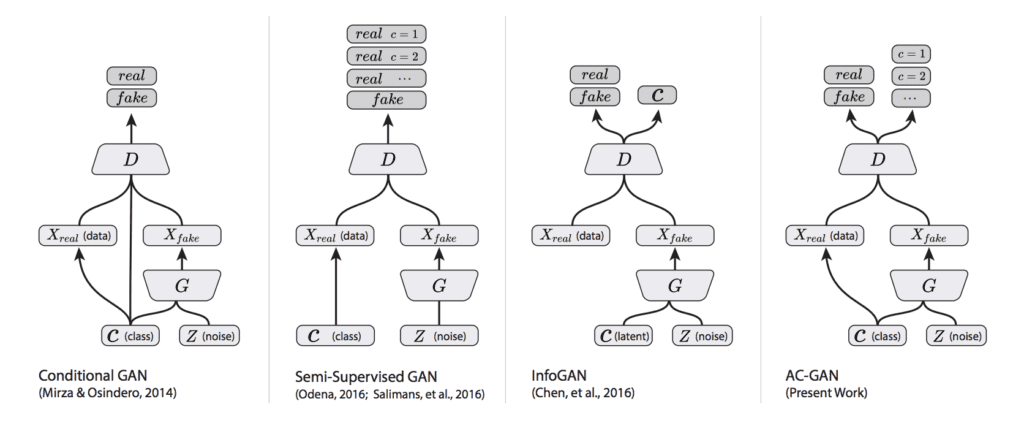
The plot below summarizes the inputs and outputs of a range of conditional GANs, including the AC-GAN, providing some context for the differences.
Summary of the Differences Between the Conditional GAN, Semi-Supervised GAN, InfoGAN, and AC-GAN. Taken from: Version of Conditional Image Synthesis With Auxiliary Classifier GANs.
The discriminator seeks to maximize the probability of correctly classifying real and fake images (LS) and correctly predicting the class label (LC) of a real or fake image (e.g. LS + LC). The generator seeks to minimize the ability of the discriminator to discriminate real and fake images whilst also maximizing the ability of the discriminator predicting the class label of real and fake images (e.g. LC – LS).
The objective function has two parts: the log-likelihood of the correct source, LS, and the log-likelihood of the correct class, LC. […] D is trained to maximize LS + LC while G is trained to maximize LC − LS.
The effect of changing the conditional GAN in this way is both a more stable training process and the ability of the model to generate higher quality images with a larger size than had been previously possible, e.g. 128×128 pixels.
… we demonstrate that adding more structure to the GAN latent space along with a specialized cost function results in higher quality samples. […] Importantly, we demonstrate quantitatively that our high resolution samples are not just naive resizings of low resolution samples.
Take my free 7-day email crash course now (with sample code).
Click to sign-up and also get a free PDF Ebook version of the course.
Fashion-MNIST Clothing Photograph Dataset
The Fashion-MNIST dataset is proposed as a more challenging replacement dataset for the MNIST handwritten digit dataset.
It is a dataset comprised of 60,000 small square 28×28 pixel grayscale images of items of 10 types of clothing, such as shoes, t-shirts, dresses, and more.
Keras provides access to the Fashion-MNIST dataset via the fashion_mnist.load_dataset() function. It returns two tuples, one with the input and output elements for the standard training dataset, and another with the input and output elements for the standard test dataset.
The example below loads the dataset and summarizes the shape of the loaded dataset.
Note: the first time you load the dataset, Keras will automatically download a compressed version of the images and save them under your home directory in ~/.keras/datasets/. The download is fast as the dataset is only about 25 megabytes in its compressed form.
1
2
3
4
5
6
7
# example of loading the fashion_mnist dataset
from keras.datasets.fashion_mnist import load_data
# load the images into memory
(trainX,trainy),(testX,testy)=load_data()
# summarize the shape of the dataset
print('Train',trainX.shape,trainy.shape)
print('Test',testX.shape,testy.shape)
Running the example loads the dataset and prints the shape of the input and output components of the train and test splits of images.
We can see that there are 60K examples in the training set and 10K in the test set and that each image is a square of 28 by 28 pixels.
1
2
Train (60000, 28, 28) (60000,)
Test (10000, 28, 28) (10000,)
The images are grayscale with a black background (0 pixel value) and the items of clothing in white ( pixel values near 255). This means if the images were plotted, they would be mostly black with a white item of clothing in the middle.
We can plot some of the images from the training dataset using the matplotlib library with the imshow() function and specify the color map via the ‘cmap‘ argument as ‘gray‘ to show the pixel values correctly.
1
2
# plot raw pixel data
pyplot.imshow(trainX[i],cmap='gray')
Alternately, the images are easier to review when we reverse the colors and plot the background as white and the clothing in black.
They are easier to view as most of the image is now white with the area of interest in black. This can be achieved using a reverse grayscale color map, as follows:
1
2
# plot raw pixel data
pyplot.imshow(trainX[i],cmap='gray_r')
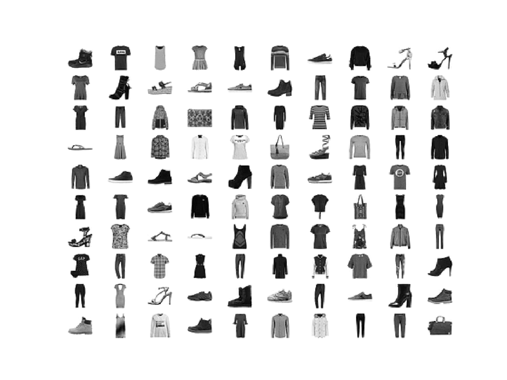
The example below plots the first 100 images from the training dataset in a 10 by 10 square.
1
2
3
4
5
6
7
8
9
10
11
12
13
14
# example of loading the fashion_mnist dataset
from keras.datasets.fashion_mnist import load_data
from matplotlib import pyplot
# load the images into memory
(trainX,trainy),(testX,testy)=load_data()
# plot images from the training dataset
foriinrange(100):
# define subplot
pyplot.subplot(10,10,1+i)
# turn off axis
pyplot.axis('off')
# plot raw pixel data
pyplot.imshow(trainX[i],cmap='gray_r')
pyplot.show()
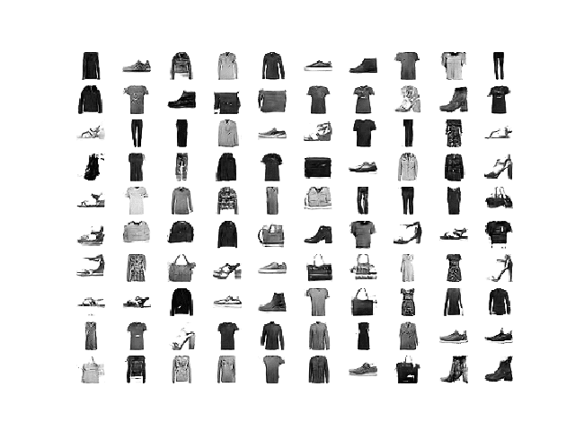
Running the example creates a figure with a plot of 100 images from the MNIST training dataset, arranged in a 10×10 square.
Plot of the First 100 Items of Clothing From the Fashion MNIST Dataset.
We will use the images in the training dataset as the basis for training a Generative Adversarial Network.
Specifically, the generator model will learn how to generate new plausible items of clothing, using a discriminator that will try to distinguish between real images from the Fashion MNIST training dataset and new images output by the generator model, and predict the class label for each.
This is a relatively simple problem that does not require a sophisticated generator or discriminator model, although it does require the generation of a grayscale output image.
How to Define AC-GAN Models
In this section, we will develop the generator, discriminator, and composite models for the AC-GAN.
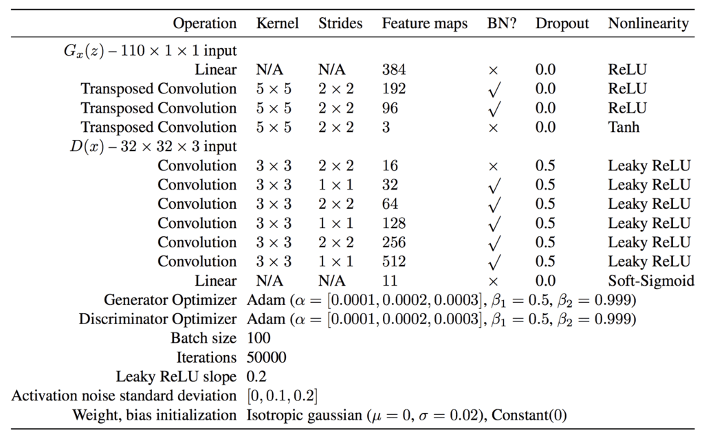
The appendix of the AC-GAN paper provides suggestions for generator and discriminator configurations that we will use as inspiration. The table below summarizes these suggestions for the CIFAR-10 dataset, taken from the paper.
AC-GAN Generator and Discriminator Model Configuration Suggestions. Take from: Conditional Image Synthesis With Auxiliary Classifier GANs.
AC-GAN Discriminator Model
Let’s start with the discriminator model.
The discriminator model must take as input an image and predict both the probability of the ‘realness‘ of the image and the probability of the image belonging to each of the given classes.
The input images will have the shape 28x28x1 and there are 10 classes for the items of clothing in the Fashion MNIST dataset.
The model can be defined as per the DCGAN architecture. That is, using Gaussian weight initialization, batch normalization, LeakyReLU, Dropout, and a 2×2 stride for downsampling instead of pooling layers.
For example, below is the bulk of the discriminator model defined using the Keras functional API.
The main difference is that the model has two output layers.
The first is a single node with the sigmoid activation for predicting the real-ness of the image.
1
2
3
...
# real/fake output
out1=Dense(1,activation='sigmoid')(fe)
The second is multiple nodes, one for each class, using the softmax activation function to predict the class label of the given image.
1
2
3
...
# class label output
out2=Dense(n_classes,activation='softmax')(fe)
We can then construct the image with a single input and two outputs.
1
2
3
...
# define model
model=Model(in_image,[out1,out2])
The model must be trained with two loss functions, binary cross entropy for the first output layer, and categorical cross-entropy loss for the second output layer.
Rather than comparing a one hot encoding of the class labels to the second output layer, as we might do normally, we can compare the integer class labels directly. We can achieve this automatically using the sparse categorical cross-entropy loss function. This will have the identical effect of the categorical cross-entropy but avoids the step of having to manually one hot encode the target labels.
When compiling the model, we can inform Keras to use the two different loss functions for the two output layers by specifying a list of function names as strings; for example:
Tying this together, the define_discriminator() function will define and compile the discriminator model for the AC-GAN.
The shape of the input images and the number of classes are parameterized and set with defaults, allowing them to be easily changed for your own project in the future.
Running the example first prints a summary of the model.
This confirms the expected shape of the input images and the two output layers, although the linear organization does make the two separate output layers clear.
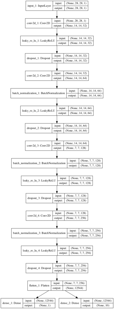
A plot of the model is also created, showing the linear processing of the input image and the two clear output layers.
Plot of the Discriminator Model for the Auxiliary Classifier GAN
Now that we have defined our AC-GAN discriminator model, we can develop the generator model.
AC-GAN Generator Model
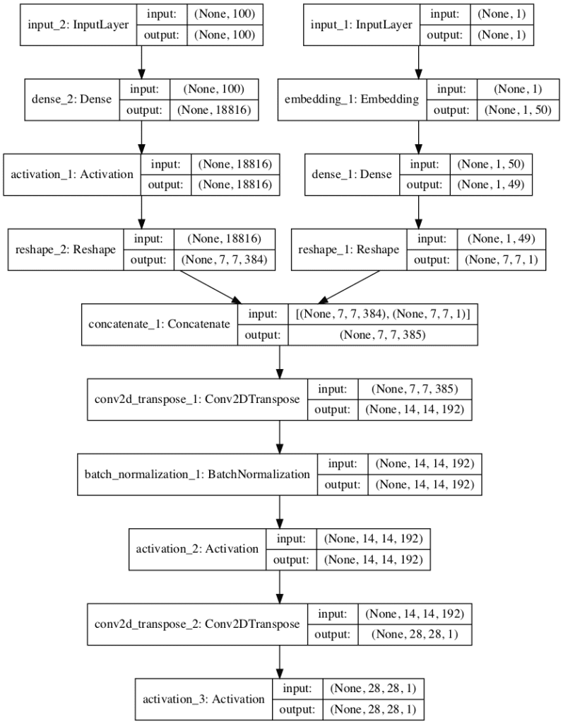
The generator model must take a random point from the latent space as input, and the class label, then output a generated grayscale image with the shape 28x28x1.
The AC-GAN paper describes the AC-GAN generator model taking a vector input that is a concatenation of the point in latent space (100 dimensions) and the one hot encoded class label (10 dimensions) that is 110 dimensions.
An alternative approach that has proven effective and is now generally recommended is to interpret the class label as an additional channel or feature map early in the generator model.
This can be achieved by using a learned embedding with an arbitrary number of dimensions (e.g. 50), the output of which can be interpreted by a fully connected layer with a linear activation resulting in one additional 7×7 feature map.
1
2
3
4
5
6
7
8
9
10
...
# label input
in_label=Input(shape=(1,))
# embedding for categorical input
li=Embedding(n_classes,50)(in_label)
# linear multiplication
n_nodes=7*7
li=Dense(n_nodes,kernel_initializer=init)(li)
# reshape to additional channel
li=Reshape((7,7,1))(li)
The point in latent space can be interpreted by a fully connected layer with sufficient activations to create multiple 7×7 feature maps, in this case, 384, and provide the basis for a low-resolution version of our output image.
The 7×7 single feature map interpretation of the class label can then be channel-wise concatenated, resulting in 385 feature maps.
These feature maps can then go through the process of two transpose convolutional layers to upsample the 7×7 feature maps first to 14×14 pixels, and then finally to 28×28 features, quadrupling the area of the feature maps with each upscaling step.
The output of the generator is a single feature map or grayscale image with the shape 28×28 and pixel values in the range [-1, 1] given the choice of a tanh activation function. We use ReLU activation for the upscaling layers instead of LeakyReLU given the suggestion the AC-GAN paper.
Running the example first prints a summary of the layers and their output shape in the model.
We can confirm that the latent dimension input is 100 dimensions and that the class label input is a single integer. We can also confirm that the output of the embedding class label is correctly concatenated as an additional channel resulting in 385 7×7 feature maps prior to the transpose convolutional layers.
The summary also confirms the expected output shape of a single grayscale 28×28 image.
A plot of the network is also created summarizing the input and output shapes for each layer.
The plot confirms the two inputs to the network and the correct concatenation of the inputs.
Plot of the Generator Model for the Auxiliary Classifier GAN
Now that we have defined the generator model, we can show how it might be fit.
AC-GAN Composite Model
The generator model is not updated directly; instead, it is updated via the discriminator model.
This can be achieved by creating a composite model that stacks the generator model on top of the discriminator model.
The input to this composite model is the input to the generator model, namely a random point from the latent space and a class label. The generator model is connected directly to the discriminator model, which takes the generated image directly as input. Finally, the discriminator model predicts both the realness of the generated image and the class label. As such, the composite model is optimized using two loss functions, one for each output of the discriminator model.
The discriminator model is updated in a standalone manner using real and fake examples, and we will review how to do this in the next section. Therefore, we do not want to update the discriminator model when updating (training) the composite model; we only want to use this composite model to update the weights of the generator model.
This can be achieved by setting the layers of the discriminator as not trainable prior to compiling the composite model. This only has an effect on the layer weights when viewed or used by the composite model and prevents them from being updated when the composite model is updated.
The define_gan() function below implements this, taking the already defined generator and discriminator models as input and defining a new composite model that can be used to update the generator model only.
1
2
3
4
5
6
7
8
9
10
11
12
13
14
# define the combined generator and discriminator model, for updating the generator
def define_gan(g_model,d_model):
# make weights in the discriminator not trainable
forlayer ind_model.layers:
ifnotisinstance(layer,BatchNormalization):
layer.trainable=False
# connect the outputs of the generator to the inputs of the discriminator
gan_output=d_model(g_model.output)
# define gan model as taking noise and label and outputting real/fake and label outputs
Now that we have defined the models used in the AC-GAN, we can fit them on the Fashion-MNIST dataset.
How to Develop an AC-GAN for Fashion-MNIST
The first step is to load and prepare the Fashion MNIST dataset.
We only require the images in the training dataset. The images are black and white, therefore we must add an additional channel dimension to transform them to be three dimensional, as expected by the convolutional layers of our models. Finally, the pixel values must be scaled to the range [-1,1] to match the output of the generator model.
The load_real_samples() function below implements this, returning the loaded and scaled Fashion MNIST training dataset ready for modeling.
1
2
3
4
5
6
7
8
9
10
11
12
# load images
def load_real_samples():
# load dataset
(trainX,trainy),(_,_)=load_data()
# expand to 3d, e.g. add channels
X=expand_dims(trainX,axis=-1)
# convert from ints to floats
X=X.astype('float32')
# scale from [0,255] to [-1,1]
X=(X-127.5)/127.5
print(X.shape,trainy.shape)
return[X,trainy]
We will require one batch (or a half batch) of real images from the dataset each update to the GAN model. A simple way to achieve this is to select a random sample of images from the dataset each time.
The generate_real_samples() function below implements this, taking the prepared dataset as an argument, selecting and returning a random sample of Fashion MNIST images and clothing class labels.
The “dataset” argument provided to the function is a list comprised of the images and class labels as returned from the load_real_samples() function. The function also returns their corresponding class label for the discriminator, specifically class=1 indicating that they are real images.
The generate_latent_points() function implements this, taking the size of the latent space as an argument and the number of points required, and returning them as a batch of input samples for the generator model. The function also returns randomly selected integers in [0,9] inclusively for the 10 class labels in the Fashion-MNIST dataset.
1
2
3
4
5
6
7
8
9
# generate points in latent space as input for the generator
Next, we need to use the points in the latent space and clothing class labels as input to the generator in order to generate new images.
The generate_fake_samples() function below implements this, taking the generator model and size of the latent space as arguments, then generating points in the latent space and using them as input to the generator model.
The function returns the generated images, their corresponding clothing class label, and their discriminator class label, specifically class=0 to indicate they are fake or generated.
1
2
3
4
5
6
7
8
9
# use the generator to generate n fake examples, with class labels
There are no reliable ways to determine when to stop training a GAN; instead, images can be subjectively inspected in order to choose a final model.
Therefore, we can periodically generate a sample of images using the generator model and save the generator model to file for later use. The summarize_performance() function below implements this, generating 100 images, plotting them, and saving the plot and the generator to file with a filename that includes the training “step” number.
1
2
3
4
5
6
7
8
9
10
11
12
13
14
15
16
17
18
19
20
21
22
# generate samples and save as a plot and save the model
The model is fit for 100 training epochs, which is arbitrary, as the model begins generating plausible items of clothing after perhaps 20 epochs. A batch size of 64 samples is used, and each training epoch involves 60,000/64, or about 937, batches of real and fake samples and updates to the model. The summarize_performance() function is called every 10 epochs, or every (937 * 10) 9,370 training steps.
For a given training step, first the discriminator model is updated for a half batch of real samples, then a half batch of fake samples, together forming one batch of weight updates. The generator is then updated via the combined GAN model. Importantly, the class label is set to 1, or real, for the fake samples. This has the effect of updating the generator toward getting better at generating real samples on the next batch.
Note, the discriminator and composite model return three loss values from the call to the train_on_batch() function. The first value is the sum of the loss values and can be ignored, whereas the second value is the loss for the real/fake output layer and the third value is the loss for the clothing label classification.
The train() function below implements this, taking the defined models, dataset, and size of the latent dimension as arguments and parameterizing the number of epochs and batch size with default arguments. The generator model is saved at the end of training.
Running the example may take some time, and GPU hardware is recommended, but not required.
Note: Your results may vary given the stochastic nature of the algorithm or evaluation procedure, or differences in numerical precision. Consider running the example a few times and compare the average outcome.
The loss is reported each training iteration, including the real/fake and class loss for the discriminator on real examples (dr), the discriminator on fake examples (df), and the generator updated via the composite model when generating images (g).
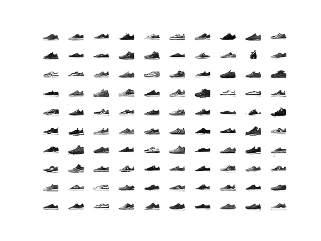
Running the example, in this case, generates 100 very plausible photos of sneakers.
Example of 100 Photos of Sneakers Generated by an AC-GAN
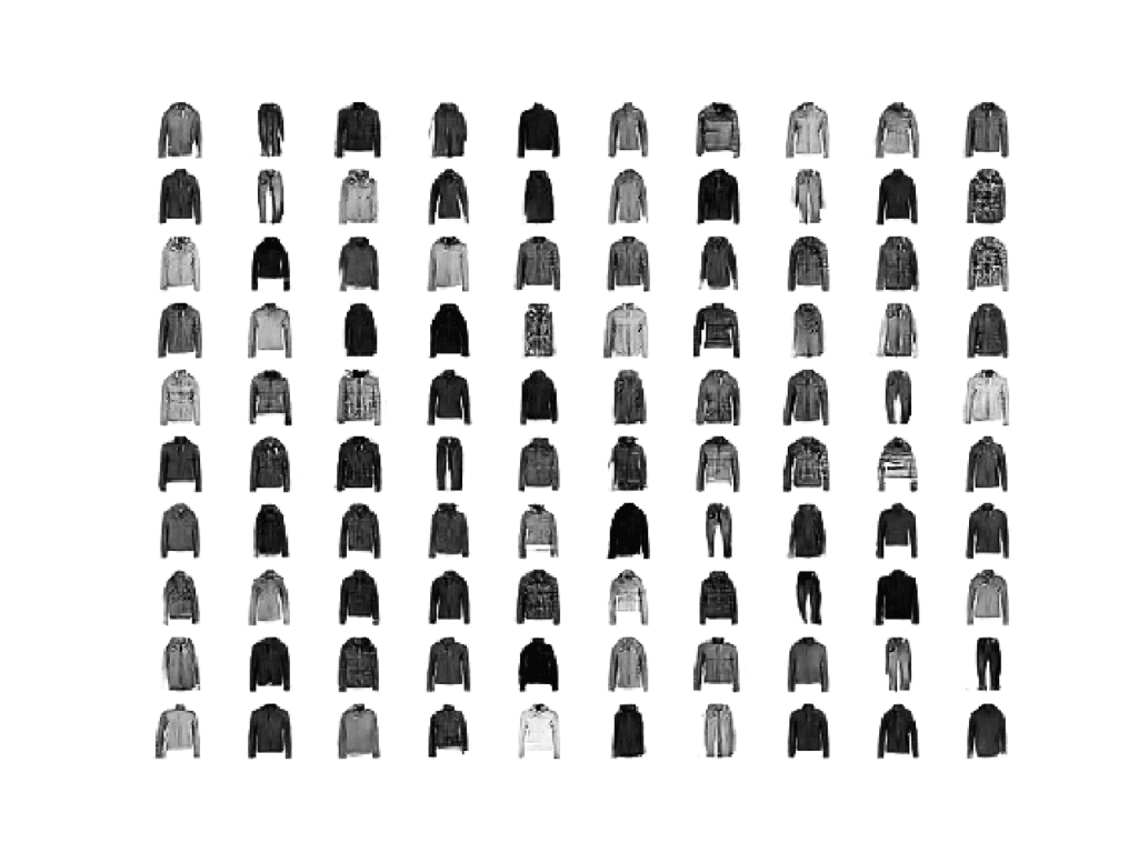
It may be fun to experiment with other class values.
For example, below are 100 generated coats (n_class = 4). Most of the images are coats, although there are a few pants in there, showing that the latent space is partially, but not completely, class-conditional.
Example of 100 Photos of Coats Generated by an AC-GAN
Extensions
This section lists some ideas for extending the tutorial that you may wish to explore.
Generate Images. Generate images for each clothing class and compare results across different saved models (e.g. epoch 10, 20, etc.).
Alternate Configuration. Update the configuration of the generator, discriminator, or both models to have more or less capacity and compare results.
CIFAR-10 Dataset. Update the example to train on the CIFAR-10 dataset and use model configuration described in the appendix of the paper.
If you explore any of these extensions, I’d love to know.
Post your findings in the comments below.
Further Reading
This section provides more resources on the topic if you are looking to go deeper.
Thank you for your excellent blogs.
One question I want to ask,Tensorflow or keras,which one do you command for realize rnn/deep-lstm/encoder-decoder/..?
I think both are good, but I don’t know how to choose.
I’m trying to get a better grasp of the latent space when “AC-GANs learn a representation for z that is independent of class label”. Does this mean that if I had a latent space in 2D, for simplicity, that the latent space does NOT have regions which are a specific class like I would in a variational autoencoder?
Thanks for your blogging Jason, you really articulate the concepts very well and your posts have helped me understand a variety of topics in machine learning.
FYI tensorflow 2.0 includes keras so I would use keras within tf2
As always, I’m very impressed with your work. I tried out your programming for the 2D graph, similar work done on LS-GAN/CGANS, and finally the AC-GAN. I confess to having to use the tensorflow version of Keras (Keras by itself doesn’t work for me for some reason). I tried out the following statement in the define_gan routine and found it did a much better job of generating correct clothing icons when tested at the end:
I like mse for exactly the reasons given with LS-GAN… In my mind, mse gives a measure of distance from the “correct” generation rather than just a measure of “correctness”.
However, I’m not sure why it would work in this problem when labels are also used. Does mse only apply to the icons and not to the labels (0 thru 9)? Hopefully I’m making sense.
I’m sure you explain it somewhere but it escapes me.
The power for deep learning show clearly in image data, but it also could serve time-series, and raw data, does not it?
Unfortunately, I can not find enough resources and examples for applying deep learning on the non-image dataset.
My question,
Does it worth to apply non-image data, raw- data set, for example, on this method?
If yes, could you kindly point me to a useful resource and guidance?
I’m actually trying to recreate it for Cifar10 using the hyperparameters given in the research paper, I see that after after a few thousand steps, the loss for discriminator for the classes of fake images goes down and fluctuates around zero, while real/fake loss stays around 0.7. I’m not sure if this means that the generator is learning something, as based on what I read discriminator loss reaching zero means it’s failure. Also, the generator loss is fluctuation around zero. Does this mean I have to restart and change the hyperparameters?
What does ‘C’ indicates in the diagram of AC-GAN?
and what is output of discriminator? It is mentioned like Probability that the provided image is real, probability of the image belonging to each known class. – What this means?
How can I check this?
I have understood the generator training part clearly,
My doubt is that, whatever losses we mention ,the model triesto mimize both.
We are writing the 2 losses i.e 1.binary cross entropy loss ( for fake or real) 2. Categorical cross entropy loss(for labels) in a similar way at 2 different places in the code(line no. 60 and 106 in the ac gan code)
at one place(line no. 60) binary cross entropy loss is supposed to be minimized (by discriminator)
and at other place (line no. 106) binary cross entropy loss is supposed to be maximized (by generator)
In tensorflow we mention a loss which to be minimized directly nad a loss which is to be maximized by negaive quantity i.e( – loss)
As you said about the order of losses from model.train_on_batch()
“Note, the discriminator and composite model return three-loss values from the call to the train_on_batch() function. The first value is the sum of the loss values and can be ignored, whereas the second value is the loss for the real/fake output layer and the third value is the loss for the clothing label classification.”
Can we apply the same order for accuracy metric also,(if we give it as a metric in discriminator)???
as I got 2 new values from model.train_on_batch(), if i give additional metric ‘accuracy’
Thank you for all of your amazing work, i am new to deep learning probably why but when i run this code, the number of steps keep going on and on, there is no sign which indicates epoch number , if these steps are iterations then they should bbe 9370 as you mentioned but in my case they are going for an infinite number can you please explain this sir that will be great..
Thank you for the response but in my case the first number represent the total number of steps which are 93750…because the number of epochs in your model are 100, with 60000 images and batch of 64 which makes 93750 steps…anyway after training i figure it out…so thank you for all of your amazing work, this site and your work is a tremendous help in my journey of deep learning especially GANs, there are not so many sources which provide both intuition and implementation, so please keep this work going you are a great help to students and researcher.
Hy! Thank you for this amazing post, i want to apply this implementation to image dataset there are only two classes male and female, i want to classify the generated images into male or female, what changes do i have to make to this code to accomplish my desired goal and.
Thank you for the response, you are a great help to many people, i will try to make some changes to this model to solve my issue, i guess i have to buy your books collection.
Dear Adrian,
Thank you for sharing your experience with us
Could you kindly tell me how to use spherical linear interpolation (slerp) to generate faces using AC gan
How will labels be treated?
Thanks in advance
When you set the d_model.trainable = False in define_gan method, I don’t see you setting it back to True anywhere. Yet it seems that when d_model is trained in isolation the weights are updated but not when the gan_model is trained. And since python argument passing is by reference, I assume d_model.trainable should be False everywhere else as well. Am I missing something?
As a student i should thank you for all your tutorials specifically for the GANs. I have a problem that I searched a lot about it but couldn’t find any helpful answer… my problem is when I use BatchNormalization layer in models, I have no improvement in training phase… and in each epoch the produced images from generator are all like the one I have in the first epoch !!! could you help me to find the solution …
Yours tutorials are just wonderfull. Thanks for them. But I have a problem with ACGAN. Every time (and believe me I tried a lot of times) I launch your code I’m getting a Convergence Failure afer about 1k iterations. What’s may be the reason of that and, what is more important, how to fix this problem?
Sorry, I wasn’t precise enough. I ran this example for 100 epochs just like you, by iterations I meant number of steps (for each epoch there are 937 steps, so Convergence Failure appears after about 1 epoch). I believe that is not too much.
Perhaps confirm that your libraries are up to date?
Perhaps try running the example many times?
Perhaps try adjusting the learning hyperparameters, e.g. learning rate?
Perhaps try adjusting the model complexity, e.g. more or fewer layers?
Perhaps try GAN hacks?
I don’t understand why, but after many tries I found the reason of Convergence Failure. After erasing all the BatchNormalization layers, model seems to work just fine. Thank you for your help. Best wishes.
Thanks for suggesting the fix to remove BatchNorm layers Radoslaw! I was facing an issue where the output was quite bad even after 100 epochs but your suggestion fixed that.
Hi Jason, thanks for the great article. I’m working on an ACGAN with a dataset of around 9000 images of 4 classes with a 256×192 resolution. I have implemented all the tips you mention here and in your other article “Tips for Training Stable Generative Adversarial Networks”. I’ve added more convolutional layers to my networks though because the images have higher resolution and the loss quickly went to zero when using your exact code. My issue is that the discriminator loss for fake images (df) is often very close to 0.. it doesn’t stay there, goes up and down quite a bit, but always comes back to around 0.00something. I’ve found that adding a smaller momentum number like 0.8 in the BatchNorm layers helps with this a little, but the problem still occurs. These are some typical values that I get:
And is there any guideline about roughly how many parameters your generator and discriminator networks should have based on the image size? Should the generator always have more parameters like in your example here?
Hi Jason, for generate_real_samples, you take a random sample of images from the data set each time. So if I understand correctly, this means that – since you take random samples – not all images from the training set may be used within one epoch, whereas some images might be used several times? I thought that in an epoch, all images in the training set needed to be used exactly once. Is it better to take random ones rather than making sure all images are used exactly once per epoch / does it not matter?
Hello,
I have tried CGAN and ACGAN on the same dataset (imbalanced) and the generated images were much realistic and diverse with CGAN. In ACGAN, for generating images with specific class, it gave me alot of realistic images from another class. Any clue on what’s happening and how do I solve it?
Hello,
Thank you for providing a great tutorial about ACGAN.
I have tried ACGAN on the human activity dataset (i.e., accelerometer) and generated synthetic data from it. However, after several times, my ACGAN still have ‘poor performance’. If I further check on the training process, the discriminator class loss on fake data is closer to zero while real/fake loss is stable.
Hi Jason, thank you for this tutorial of ACGAN. My problem / question is that can we use this network for audio generation, speech command to be exact ? I tried to do this with mel-spectrograms of command set but could obtain any acceptable result. I am wondering if it’s possible to obtain any good results with this kind of network or if it’s a dead end.
What is your opinion on this ?
Thanks.
Thanks for this post, it was really interesting.
I followed along and tried to run the code for the Fashion-MNiST dataset but my results are much worse than the ones you managed to produce.
The images generated after training a model for 100 epochs look like this – https://ibb.co/Tv90c25
Could please help me out on how I can improve this to match yours? Any help is greatly appreciated.
And his solution of removing the BatchNormalization layers from both Generator and Discriminator worked and fixed the problem. Now my results look pretty good after just 10 epochs as noted by you.
Thanks again and if you want you may add a small edit to the post or disclaimer to remove BatchNorm layers.
One thing I’m not sure of is why removing BatchNorm layers helped and improved the output in this case? Do you have any ideas or thoughts on this?
Ok i have plotted datapoints looks fine after 15k epoch don’t see mode collapse. I have one interesting result, the overall discriminator model accuracy is decreasing which is expected, however i also discriminator classifier is also poorly performing over the iterations. As per our understanding classifier should be good enough to classify as we progress ?
After 100 epochs, I manage to obtain a classification accuracy on the training set (413 images) of around 80%, but the testing accuracy is very low. Here is an example of the generated image by the generator model: https://ibb.co/FDZ6ZxQ. Would you like to guide me to improve the testing accuracy?
Perhaps try tuning the model architecture or learning parametres to see if it makes a difference?
Perhaps try preparing the image data in alternate ways, e.g. standardising vs normalizing?
Currently, I haven’t tried to tune the parameters and still use the default learning parameter values as yours. I suppose you are correct and I will try to tune them later.
But my current concern is: do I need to improve the generator model than that of yours since I work with RGB images that also have larger sizes than the images you used in this tutorial?
Perhaps I need to improve the discriminator capacity as well?
Hi,
Thank you for your post, it is really helpful! I am trying to create an AC-GAN for a project and I would like to ask if my concatenation of the label and the latent space is ok for the generator to learn different labels, as currently it is outputting the same image for all labels.
When I am trying to use the final Model “How to Generate Items of Clothing With the AC-GAN”
I get this error message
USEMODELAC.py:23: MatplotlibDeprecationWarning: Passing non-integers as three-element position specification is deprecated since 3.3 and will be removed two minor releases later.
pyplot.subplot(sqrt(n_examples), sqrt(n_examples), 1 + i)
Can anyone or mr Brownlee can you help em what to do?
Hello,
When I am running the code I get losses equal to zero for real/fake discriminator for all three of them while the class classifier is around 1.0 for all three. Is that failure mode even though I am on the 3 epoch? Which parameters should I try changing?
Perhaps continue training and review the results.
Perhaps try adjusting the model configuration.
Perhaps try adjusting the learning hyperparameters.
Perhaps ensure your libraries are up to date.
Hallo Jason,
thank you for everything!
I just have a question. Is this a supervised or a semi-supervised learning?
if it’s semi where is the unlabeled data in this case.
Thanks a lot.
This is a super helpful tutorial. I wanted to ask how much memory this network generally takes to effectively run?
I have a low parameter count for my generator and discriminator, yet it still seems to run out of memory. I do have a custom implementation where my images are about 4 times the size, however I still run out of memory even with a batch size of 1.
I’m using two GPUs simultaneously: Nvidia GTX 2060 and 2070.
Any thoughts on why I would be running out of memory with this GAN network, but have no problem on a standard CNN or Autoencoder?
Very explanatory example.
I got a question like what ill be the y_true and y_pred in case of generator loss computation.
I have been trying to modify the loss function. It is giving me different dimension for y_true and y_pred.
Your response will be much appreciated.
The loss function would not change the dimension (only the value can change as you’re now optimizing for a different thing), but changing the model output would. Can you check?
I did not add a new ouput; but using binarycrossentropy and sparse categorical cross entropy as in ACGAN.
While adding the custom sparse categorical cross entropy, the y_true and y_pred is like (batch_size, 1) and (batchsize, no.of classes)respectively; I applied reduction to sparse CE, still the dimension remains like this.
Whereas when I use the loss = [‘binary_crossentropy’, ‘sparse_categorical_crossentropy’], the dimension the y_true and y_pred is like (batch_size, 1) and (batchsize, 1) respectively.
That means your y_true is not in one-hot encoding while your y_pred is. So simply, convert your y_true before you feed into the loss function would solve it.
Hey! As stated above, I’ve been working on turning this GAN into something that can be used on the CIFAR-10 database. I think I have changed all the relevant parts but my model is consistently suffering from Mode Collapse when I run it. How can I avoid this?
Hi James, I’ve had a similar issue as AM (mode collapse on CIFAR-10 ac-gan based off this tutorial) and I read through the article you suggested. It seems to focus more on the identification of Mode Collapse (which I have accomplished) and I couldn’t find any tips to remedy it. What would be some ways to fix the mode collapse (I’m not sure if this is relevant but I used the configurations suggested by Conditional Image Synthesis With Auxiliary Classifier GANs from the table in the “How to Define AC-GAN Models” section of this tutorial)?
I’m eager to help, but I just don’t have the capacity to debug code for you.
I am happy to make some suggestions:
Consider aggressively cutting the code back to the minimum required. This will help you isolate the problem and focus on it.
Consider cutting the problem back to just one or a few simple examples.
Consider finding other similar code examples that do work and slowly modify them to meet your needs. This might expose your misstep.
Consider posting your question and code to StackOverflow.
amazing work , i just have one question when i am training AC GAN on my dataset having 11 classes , then when i am saving generator model and outputing images , then when i give class_label as 2 or 2000 , it still gives ouput ,how is that so when i have only 11 classes
Hi Avinash…I appreciate the feedback and support! Could you possibly rephrase or elaborate on your question so that we may better assist you. Perhaps you could share a code sample listing.
hello james , thanks or the reply . It means a lot .My ques was :- suppose i train my acgan and save my generator model .Now i will use my generator to produce images , but i want that when i give class label as class 2 , my generator shd produce images of class 2 but in my case , even if i am giving input as class label 2000 (which is wrong as it have only 11 classes) , it is still producing images .How is it behaving this way
Hi. Thanks for your blogging Jason, is “kernel_initializer = init” necessary in the discriminator? And what is the reason for its existence in the ACGAN?
In the figure of “Summary of the Differences Between the CGAN & ACGAN”, I see a directional arrow going from ‘C’ to ‘X Real (data)’ in both, CGAN and ACGAN.
What does this mean?
That is, the original data enters to the discriminator with their own original label?
hello james , thanks or the reply . It means a lot .My ques was :- suppose i train my acgan and save my generator model .Now i will use my generator to produce images , but i want that when i give class label as class 2 , my generator shd produce images of class 2 but in my case , even if i am giving input as class label 2000 (which is wrong as it have only 11 classes) , it is still producing images .How is it behaving this way
i dont understand in the train() where you use gan_model to train but use g_model to pass in summarize_performance() when it’s just passed in the function not training anything but the gan_model is trained but not use anywhere?
Hi can you explain the train function for me? Why the gan_model is trained but the g_model is used for summarize_performance? when the g_model is just a created model in the begining it’s not trained in the train function so im confused.


 in Keras")
 From Scratch")

 From Scratch in Keras")


Thank you for your excellent blogs.
One question I want to ask,Tensorflow or keras,which one do you command for realize rnn/deep-lstm/encoder-decoder/..?
I think both are good, but I don’t know how to choose.
Thanks again
Keras.
Thanks for the great article! 🙂
I’m trying to get a better grasp of the latent space when “AC-GANs learn a representation for z that is independent of class label”. Does this mean that if I had a latent space in 2D, for simplicity, that the latent space does NOT have regions which are a specific class like I would in a variational autoencoder?
It does not force or guarantee the mapping or association, but it will capture something that makes sense to the model for image synthesis.
For real control, use a conditional GAN or an InfoGAN.
Thanks for your blogging Jason, you really articulate the concepts very well and your posts have helped me understand a variety of topics in machine learning.
FYI tensorflow 2.0 includes keras so I would use keras within tf2
Thanks for your support.
TF2 is not released, it is in beta. I recommend standalone keras at this stage.
As always, I’m very impressed with your work. I tried out your programming for the 2D graph, similar work done on LS-GAN/CGANS, and finally the AC-GAN. I confess to having to use the tensorflow version of Keras (Keras by itself doesn’t work for me for some reason). I tried out the following statement in the define_gan routine and found it did a much better job of generating correct clothing icons when tested at the end:
model.compile(loss=[‘mse’, ‘sparse_categorical_crossentropy’], optimizer=opt)
I like mse for exactly the reasons given with LS-GAN… In my mind, mse gives a measure of distance from the “correct” generation rather than just a measure of “correctness”.
However, I’m not sure why it would work in this problem when labels are also used. Does mse only apply to the icons and not to the labels (0 thru 9)? Hopefully I’m making sense.
I’m sure you explain it somewhere but it escapes me.
Thanks for your great work.
Thanks.
Nice one! Yes, I’m a big fan of MSE loss, it’s also used heavily on fancy GANs like pix2pix and cyclegan.
Thanks for your excellent blogging Jason,
The power for deep learning show clearly in image data, but it also could serve time-series, and raw data, does not it?
Unfortunately, I can not find enough resources and examples for applying deep learning on the non-image dataset.
My question,
Does it worth to apply non-image data, raw- data set, for example, on this method?
If yes, could you kindly point me to a useful resource and guidance?
Thank you in advance,
Yes, see here:
https://machinelearningmastery.com/start-here/#deep_learning_time_series
And it does great on text data:
https://machinelearningmastery.com/start-here/#nlp
Thank you for the neatly explained article Jason,
I’m actually trying to recreate it for Cifar10 using the hyperparameters given in the research paper, I see that after after a few thousand steps, the loss for discriminator for the classes of fake images goes down and fluctuates around zero, while real/fake loss stays around 0.7. I’m not sure if this means that the generator is learning something, as based on what I read discriminator loss reaching zero means it’s failure. Also, the generator loss is fluctuation around zero. Does this mean I have to restart and change the hyperparameters?
Thanks again in advance
It likely suggests a gan failure mode:
https://machinelearningmastery.com/practical-guide-to-gan-failure-modes/
Yes, restart.
How to predict the class label of a given image?
GANs are not used for image classification, instead you can use different models described here:
https://machinelearningmastery.com/start-here/#dlfcv
What does ‘C’ indicates in the diagram of AC-GAN?
and what is output of discriminator? It is mentioned like Probability that the provided image is real, probability of the image belonging to each known class. – What this means?
How can I check this?
C is the class.
The output of the discriminator is whether the image is real or fake. If this is a new idea, perhaps start with the simpler tutorials here:
https://machinelearningmastery.com/start-here/#gans
Hi sir, but you said that AC gan can predict the class of a given image, what does this mean?
It means that the model is trained on data where images are labeled.
Thanks for you wonderful blogs and your GAN book Jason,
kindly help me in understanding this much better.
y doubt is how the loss of AC GAN i.e “LC-LS” can be interpreted from the loss functions in “define GAN()” funtion
if the below code determines LC +LS in discriminator :
model.compile(loss=[‘binary_crossentropy’, ‘sparse_categorical_crossentropy’], optimizer=opt)
(real images y=1, fake images y=0)
How the below code determines LC- LS in generator training :???
model.compile(loss=[‘binary_crossentropy’, ‘sparse_categorical_crossentropy’], optimizer=opt)
(fake images y=1)
Recall that the generator is updated via the discriminator.
I have understood the generator training part clearly,
My doubt is that, whatever losses we mention ,the model triesto mimize both.
We are writing the 2 losses i.e 1.binary cross entropy loss ( for fake or real) 2. Categorical cross entropy loss(for labels) in a similar way at 2 different places in the code(line no. 60 and 106 in the ac gan code)
at one place(line no. 60) binary cross entropy loss is supposed to be minimized (by discriminator)
and at other place (line no. 106) binary cross entropy loss is supposed to be maximized (by generator)
In tensorflow we mention a loss which to be minimized directly nad a loss which is to be maximized by negaive quantity i.e( – loss)
can you please clear this doubt?
Yes, we fit the generator via the discriminator here. The input passes through the discriminator to the generator.
Perhaps start with this tutorial to better understand the chosen architecture for model updates:
https://machinelearningmastery.com/how-to-develop-a-generative-adversarial-network-for-a-1-dimensional-function-from-scratch-in-keras/
Hi jason,
if try to print accuracy also for final gan model , there are total 5 parametrs in output of model.compile()
loss1+loss2, loss1, loss2, accuracy1, accuracy2
you have explained about the out when compiled using only loss, saying
loss1 –for real/fake
loss2– for labels
so can i derive that
accuracy– for real/fake (ofcourse it has no meaning)
accuracy2– for labels ?????????????
Accuracy of the classifier is most relevant, the discriminator less so.
As you said about the order of losses from model.train_on_batch()
“Note, the discriminator and composite model return three-loss values from the call to the train_on_batch() function. The first value is the sum of the loss values and can be ignored, whereas the second value is the loss for the real/fake output layer and the third value is the loss for the clothing label classification.”
Can we apply the same order for accuracy metric also,(if we give it as a metric in discriminator)???
as I got 2 new values from model.train_on_batch(), if i give additional metric ‘accuracy’
Thank you so much for your replies Jason!
Yes, I believe so.
How to get the accuracy of the classifier? I want to know how well the model has predicted the class labels.
We don’t measure the accuracy of GANs, instead we score their generated images:
https://machinelearningmastery.com/how-to-evaluate-generative-adversarial-networks/
Hi Jason,
Have you implemented keras acgan code with Wasserstein metric? Would be of great help.
This (above) is the only implementation of the AC-GAN I have.
Thank you for all of your amazing work, i am new to deep learning probably why but when i run this code, the number of steps keep going on and on, there is no sign which indicates epoch number , if these steps are iterations then they should bbe 9370 as you mentioned but in my case they are going for an infinite number can you please explain this sir that will be great..
>18290, dr[0.317,0.741], df[0.474,0.061], g[1.949,0.154]
>18291, dr[0.236,1.152], df[0.341,0.093], g[2.630,0.043]
>1829, dr[0.477,0.674], df[0.441,0.143], g[2.447,0.097]
>18293, dr[0.622,0.789], df[0.402,0.134], g[2.926,0.076]
The first number will be the epoch number.
Thank you for the response but in my case the first number represent the total number of steps which are 93750…because the number of epochs in your model are 100, with 60000 images and batch of 64 which makes 93750 steps…anyway after training i figure it out…so thank you for all of your amazing work, this site and your work is a tremendous help in my journey of deep learning especially GANs, there are not so many sources which provide both intuition and implementation, so please keep this work going you are a great help to students and researcher.
Happy to hear that you figured out your issue!
Hy! Thank you for this amazing post, i want to apply this implementation to image dataset there are only two classes male and female, i want to classify the generated images into male or female, what changes do i have to make to this code to accomplish my desired goal and.
Kind Regards
Not a lot. Use your dataset instead of my dataset, perhaps tune the models a little. Change to binary cross entropy – for your 2 classes.
Thank you for the response, you are a great help to many people, i will try to make some changes to this model to solve my issue, i guess i have to buy your books collection.
You’re welcome.
Can the GANs predict the label of the image rather than generating images
Some can, but they are designed to generate images. This is their purpose.
Tnq Jason. Can you suggest some GANs that can be used in Predictive Analytics
GANs are generally not used for prediction, they are generative models.
Dear Adrian,
Thank you for sharing your experience with us
Could you kindly tell me how to use spherical linear interpolation (slerp) to generate faces using AC gan
How will labels be treated?
Thanks in advance
Adrian?
Thanks for the suggestion, perhaps I will cover the topic in the future.
Dear Jason,
I am really sorry for this conflict
No problem.
When you set the d_model.trainable = False in define_gan method, I don’t see you setting it back to True anywhere. Yet it seems that when d_model is trained in isolation the weights are updated but not when the gan_model is trained. And since python argument passing is by reference, I assume d_model.trainable should be False everywhere else as well. Am I missing something?
No need as it only impact the composite model.
To learn more about how freezing layers works, see this:
“How can I freeze layers and do fine-tuning?”
https://keras.io/getting_started/faq/#how-can-i-freeze-layers-and-do-fine-tuning
As a student i should thank you for all your tutorials specifically for the GANs. I have a problem that I searched a lot about it but couldn’t find any helpful answer… my problem is when I use BatchNormalization layer in models, I have no improvement in training phase… and in each epoch the produced images from generator are all like the one I have in the first epoch !!! could you help me to find the solution …
You’re welcome.
Perhaps you can try an alternate model configuration or learning configuration and find an approach that best suits your dataset.
Hi Jason,
Yours tutorials are just wonderfull. Thanks for them. But I have a problem with ACGAN. Every time (and believe me I tried a lot of times) I launch your code I’m getting a Convergence Failure afer about 1k iterations. What’s may be the reason of that and, what is more important, how to fix this problem?
Thanks in advance for your response.
Why train so long?
Train for far fewer epochs and keep on the generated images.
Also, these tips may help avoid mode failure / convergence:
https://machinelearningmastery.com/how-to-code-generative-adversarial-network-hacks/
Sorry, I wasn’t precise enough. I ran this example for 100 epochs just like you, by iterations I meant number of steps (for each epoch there are 937 steps, so Convergence Failure appears after about 1 epoch). I believe that is not too much.
Thanks.
Perhaps confirm that your libraries are up to date?
Perhaps try running the example many times?
Perhaps try adjusting the learning hyperparameters, e.g. learning rate?
Perhaps try adjusting the model complexity, e.g. more or fewer layers?
Perhaps try GAN hacks?
I don’t understand why, but after many tries I found the reason of Convergence Failure. After erasing all the BatchNormalization layers, model seems to work just fine. Thank you for your help. Best wishes.
Well done, I’m happy to hear that.
Also, no one has a good idea of the “why” questions for GANs 🙂
Thanks for suggesting the fix to remove BatchNorm layers Radoslaw! I was facing an issue where the output was quite bad even after 100 epochs but your suggestion fixed that.
Thank you!
Hi Jason, thanks for the great article. I’m working on an ACGAN with a dataset of around 9000 images of 4 classes with a 256×192 resolution. I have implemented all the tips you mention here and in your other article “Tips for Training Stable Generative Adversarial Networks”. I’ve added more convolutional layers to my networks though because the images have higher resolution and the loss quickly went to zero when using your exact code. My issue is that the discriminator loss for fake images (df) is often very close to 0.. it doesn’t stay there, goes up and down quite a bit, but always comes back to around 0.00something. I’ve found that adding a smaller momentum number like 0.8 in the BatchNorm layers helps with this a little, but the problem still occurs. These are some typical values that I get:
>526, dr[0.863,4.146], df[0.016,0.797], g[1.441,1.510]
>527, dr[0.485,5.122], df[0.001,0.432], g[1.107,1.458]
>528, dr[0.714,6.939], df[0.000,0.134], g[2.428,2.347]
>529, dr[1.288,6.916], df[0.440,1.296], g[1.442,1.757]
>530, dr[1.151,6.066], df[0.568,2.175], g[0.973,1.084]
>531, dr[0.714,3.896], df[0.001,1.817], g[2.965,0.757]
Any idea what parameter I should tweak to make this more stable? Or could the training set be too small?
Thanks so much, your articles have been extremely helpful!
And is there any guideline about roughly how many parameters your generator and discriminator networks should have based on the image size? Should the generator always have more parameters like in your example here?
Not really, lots of trial and error in configuring GANs.
Well done!
Perhaps model stability does not matter? (e.g. focus on the generated images)
Perhaps a larger model?
Perhaps a smaller learning rate?
Hi Jason, for generate_real_samples, you take a random sample of images from the data set each time. So if I understand correctly, this means that – since you take random samples – not all images from the training set may be used within one epoch, whereas some images might be used several times? I thought that in an epoch, all images in the training set needed to be used exactly once. Is it better to take random ones rather than making sure all images are used exactly once per epoch / does it not matter?
Correct. I chose this approach for simplicity and consistency with all my other GAN tutorials.
Yes, you can change it to shuffle the dataset prior to each epoch and enumerate all images.
I don’t think it will matter much, but happy to be proven wrong.
Hello,
I have tried CGAN and ACGAN on the same dataset (imbalanced) and the generated images were much realistic and diverse with CGAN. In ACGAN, for generating images with specific class, it gave me alot of realistic images from another class. Any clue on what’s happening and how do I solve it?
Nice work!
Perhaps you need to tune the model for your dataset.
Hello,
Thank you for providing a great tutorial about ACGAN.
I have tried ACGAN on the human activity dataset (i.e., accelerometer) and generated synthetic data from it. However, after several times, my ACGAN still have ‘poor performance’. If I further check on the training process, the discriminator class loss on fake data is closer to zero while real/fake loss is stable.
2020-11-23 21:54:07.524759
————— AC-GAN TRAINING —————
>10, >10, dr[0.684,1.590], df[0.793,1.600], g[0.415,1.576]
>20, >10, dr[0.633,1.581], df[0.725,1.595], g[0.619,1.630]
>30, >10, dr[0.701,1.475], df[0.473,0.388], g[0.959,0.417]
>40, >10, dr[0.725,0.920], df[0.591,0.112], g[0.376,0.111]
>50, >10, dr[0.686,0.915], df[0.642,0.023], g[0.444,0.050]
>60, >10, dr[0.846,0.470], df[0.711,0.025], g[0.566,0.085]
>70, >10, dr[0.805,0.761], df[0.744,0.022], g[0.593,0.031]
>80, >10, dr[0.670,0.623], df[0.695,0.018], g[0.678,0.021]
>90, >10, dr[0.683,0.552], df[0.687,0.005], g[0.698,0.005]
>100, >10, dr[0.646,0.595], df[0.779,0.050], g[0.646,0.018]
>110, >10, dr[0.648,0.530], df[0.674,0.000], g[0.804,0.002]
Do you have any clues on what’s happening and how do I solve it?
Thanks.
Perhaps try varying the model configurations to see if it has an impact on the quality of generated data.
Hi Jason, thank you for this tutorial of ACGAN. My problem / question is that can we use this network for audio generation, speech command to be exact ? I tried to do this with mel-spectrograms of command set but could obtain any acceptable result. I am wondering if it’s possible to obtain any good results with this kind of network or if it’s a dead end.
What is your opinion on this ?
Thanks.
I don’t think so, it is designed for image data.
Perhaps check the literature for GANs that are appropriate for audio data.
Hello Jason,
Thanks for this post, it was really interesting.
I followed along and tried to run the code for the Fashion-MNiST dataset but my results are much worse than the ones you managed to produce.
The images generated after training a model for 100 epochs look like this – https://ibb.co/Tv90c25
Could please help me out on how I can improve this to match yours? Any help is greatly appreciated.
Thanks.
You might need to run the example a few times to get good results.
Hi Jason,
Thanks for the quick response. I did run the model a few times and the result was the same.
But, I went through each of the comments on this post to see if anyone was facing the same issue and tried the fix that Radoslaw has mentioned above (link to the comment here for future ref – https://machinelearningmastery.com/how-to-develop-an-auxiliary-classifier-gan-ac-gan-from-scratch-with-keras/#comment-559908)
And his solution of removing the BatchNormalization layers from both Generator and Discriminator worked and fixed the problem. Now my results look pretty good after just 10 epochs as noted by you.
Thanks again and if you want you may add a small edit to the post or disclaimer to remove BatchNorm layers.
One thing I’m not sure of is why removing BatchNorm layers helped and improved the output in this case? Do you have any ideas or thoughts on this?
Thanks, I’ll investigate.
If the result looks better or evaluates better by modifying the architecture (depending on your goals), then the modification is good.
Does AC GAN too suffer mode collapse which we see in GAN.
It can, but it seems less common. The additional model/prediction appears to add some stability (or I’m biased in my experiments – which is possible).
Ok i have plotted datapoints looks fine after 15k epoch don’t see mode collapse. I have one interesting result, the overall discriminator model accuracy is decreasing which is expected, however i also discriminator classifier is also poorly performing over the iterations. As per our understanding classifier should be good enough to classify as we progress ?
If the performance of your model is not sufficient, perhaps your model requires further tuning?
Hi Jason,
an excellent tutorial from you, as usual.
Now, I am trying to adapt your code to classify RGB images into 5 classes. I set the input shape to (224,224,3) as the original RGB image has a large resolution (around 4000×2000 pixels). Here is an example of the original RGB image: https://grand-challenge-public.s3.amazonaws.com/f/challenge/183/f7be082d-501d-4ac2-a072-b8afc82e551a/sample.jpg.
After 100 epochs, I manage to obtain a classification accuracy on the training set (413 images) of around 80%, but the testing accuracy is very low. Here is an example of the generated image by the generator model: https://ibb.co/FDZ6ZxQ. Would you like to guide me to improve the testing accuracy?
Well done.
Perhaps try tuning the model architecture or learning parametres to see if it makes a difference?
Perhaps try preparing the image data in alternate ways, e.g. standardising vs normalizing?
Thanks for your prompt reply, Jason.
Currently, I haven’t tried to tune the parameters and still use the default learning parameter values as yours. I suppose you are correct and I will try to tune them later.
But my current concern is: do I need to improve the generator model than that of yours since I work with RGB images that also have larger sizes than the images you used in this tutorial?
Perhaps I need to improve the discriminator capacity as well?
Thanks in advance.
Perhaps. We cannot know off the cuff. I recommend experimenting and discover the answer.
Hi,
Thank you for your post, it is really helpful! I am trying to create an AC-GAN for a project and I would like to ask if my concatenation of the label and the latent space is ok for the generator to learn different labels, as currently it is outputting the same image for all labels.
input_latent = Input(shape=(z_size,))
input_label = Input(shape=(1,))
in_label = Dense(z_size)(input_label)
merged = Concatenate()([input_latent, in_label])
merged = Dense(z_size)(merged)
model_gen = layers.Reshape(target_shape=(1,z_size,))(merged)
Sorry, I don’t have the capacity to review/debug your code, I hope you can understand.
Perhaps you can use the above tutorial example as a starting point and adapt it for your dataset.
Hey,
When I am trying to use the final Model “How to Generate Items of Clothing With the AC-GAN”
I get this error message
USEMODELAC.py:23: MatplotlibDeprecationWarning: Passing non-integers as three-element position specification is deprecated since 3.3 and will be removed two minor releases later.
pyplot.subplot(sqrt(n_examples), sqrt(n_examples), 1 + i)
Can anyone or mr Brownlee can you help em what to do?
You can safely ignore this warning for now.
Hello,
When I am running the code I get losses equal to zero for real/fake discriminator for all three of them while the class classifier is around 1.0 for all three. Is that failure mode even though I am on the 3 epoch? Which parameters should I try changing?
It might be.
Perhaps continue training and review the results.
Perhaps try adjusting the model configuration.
Perhaps try adjusting the learning hyperparameters.
Perhaps ensure your libraries are up to date.
Hallo Jason,
thank you for everything!
I just have a question. Is this a supervised or a semi-supervised learning?
if it’s semi where is the unlabeled data in this case.
Thanks a lot.
best regards
Amal
It’s a mix.
What is the difference between the semi supervised learning and this model. I am trying to do a comparison.
Thanks
Perhaps this will help:
https://machinelearningmastery.com/what-is-semi-supervised-learning/
Hi Jason,
This is a super helpful tutorial. I wanted to ask how much memory this network generally takes to effectively run?
I have a low parameter count for my generator and discriminator, yet it still seems to run out of memory. I do have a custom implementation where my images are about 4 times the size, however I still run out of memory even with a batch size of 1.
I’m using two GPUs simultaneously: Nvidia GTX 2060 and 2070.
Any thoughts on why I would be running out of memory with this GAN network, but have no problem on a standard CNN or Autoencoder?
Thank you for all that you do!
Lucas
I don’t know off hand, sorry.
The problem was resolved!
Please disregard.
Happy to hear that.
Hi Jason,
Very explanatory example.
I got a question like what ill be the y_true and y_pred in case of generator loss computation.
I have been trying to modify the loss function. It is giving me different dimension for y_true and y_pred.
Your response will be much appreciated.
Thanks in advance
The loss function would not change the dimension (only the value can change as you’re now optimizing for a different thing), but changing the model output would. Can you check?
Hi Adrian Tam,
I did not add a new ouput; but using binarycrossentropy and sparse categorical cross entropy as in ACGAN.
While adding the custom sparse categorical cross entropy, the y_true and y_pred is like (batch_size, 1) and (batchsize, no.of classes)respectively; I applied reduction to sparse CE, still the dimension remains like this.
Whereas when I use the loss = [‘binary_crossentropy’, ‘sparse_categorical_crossentropy’], the dimension the y_true and y_pred is like (batch_size, 1) and (batchsize, 1) respectively.
I couldnt figure out if this is correct or not?
That means your y_true is not in one-hot encoding while your y_pred is. So simply, convert your y_true before you feed into the loss function would solve it.
Ok, Got it now.
Thanks you for the help.
The way the network is trained and the loss function is totally wrong.
read Acgan article then you will realize that this code is wrong
Hi
Thank you for the tutorial.
I’ve been trying to implement your code to work on a 1D dataset but i keep getting this error:
ValueError: Layer “model_30” expects 1 input(s), but it received 2 input tensors. Inputs received: [, ]
Any ideas?
Hammam
ValueError: Layer “model_30” expects 1 input(s), but it received 2 input tensors. Inputs received: [, ]
Surely you need to check your input size to the model.
Hey! As stated above, I’ve been working on turning this GAN into something that can be used on the CIFAR-10 database. I think I have changed all the relevant parts but my model is consistently suffering from Mode Collapse when I run it. How can I avoid this?
Hi AM…Please refer to the following:
https://machinelearningmastery.com/practical-guide-to-gan-failure-modes/
Hi James, I’ve had a similar issue as AM (mode collapse on CIFAR-10 ac-gan based off this tutorial) and I read through the article you suggested. It seems to focus more on the identification of Mode Collapse (which I have accomplished) and I couldn’t find any tips to remedy it. What would be some ways to fix the mode collapse (I’m not sure if this is relevant but I used the configurations suggested by Conditional Image Synthesis With Auxiliary Classifier GANs from the table in the “How to Define AC-GAN Models” section of this tutorial)?
Hi Jerry…Thanks for asking.
I’m eager to help, but I just don’t have the capacity to debug code for you.
I am happy to make some suggestions:
Consider aggressively cutting the code back to the minimum required. This will help you isolate the problem and focus on it.
Consider cutting the problem back to just one or a few simple examples.
Consider finding other similar code examples that do work and slowly modify them to meet your needs. This might expose your misstep.
Consider posting your question and code to StackOverflow.
hello james ,
amazing work , i just have one question when i am training AC GAN on my dataset having 11 classes , then when i am saving generator model and outputing images , then when i give class_label as 2 or 2000 , it still gives ouput ,how is that so when i have only 11 classes
Hi Avinash…I appreciate the feedback and support! Could you possibly rephrase or elaborate on your question so that we may better assist you. Perhaps you could share a code sample listing.
hello james , thanks or the reply . It means a lot .My ques was :- suppose i train my acgan and save my generator model .Now i will use my generator to produce images , but i want that when i give class label as class 2 , my generator shd produce images of class 2 but in my case , even if i am giving input as class label 2000 (which is wrong as it have only 11 classes) , it is still producing images .How is it behaving this way
Hi. Thanks for your blogging Jason, is “kernel_initializer = init” necessary in the discriminator? And what is the reason for its existence in the ACGAN?
In the figure of “Summary of the Differences Between the CGAN & ACGAN”, I see a directional arrow going from ‘C’ to ‘X Real (data)’ in both, CGAN and ACGAN.
What does this mean?
That is, the original data enters to the discriminator with their own original label?
hello james , thanks or the reply . It means a lot .My ques was :- suppose i train my acgan and save my generator model .Now i will use my generator to produce images , but i want that when i give class label as class 2 , my generator shd produce images of class 2 but in my case , even if i am giving input as class label 2000 (which is wrong as it have only 11 classes) , it is still producing images .How is it behaving this way
how can I know the accuracy of gan?
how do draw G-loss and D-loss, I can’t add a model.fit() to draw the figure appears the converge of training
HI how can i detect in AC-GAN if you have any other links plzz share
Hi Naveed…Please clarify what is meant by “detect in AC-GAN” so that we may better assist you.
i dont understand in the train() where you use gan_model to train but use g_model to pass in summarize_performance() when it’s just passed in the function not training anything but the gan_model is trained but not use anywhere?
Hi Alex…The following location is a great starting point for GANs
https://machinelearningmastery.com/start-here/#gans
Hi can you explain the train function for me? Why the gan_model is trained but the g_model is used for summarize_performance? when the g_model is just a created model in the begining it’s not trained in the train function so im confused.