The Least Squares Generative Adversarial Network, or LSGAN for short, is an extension to the GAN architecture that addresses the problem of vanishing gradients and loss saturation.
It is motivated by the desire to provide a signal to the generator about fake samples that are far from the discriminator model’s decision boundary for classifying them as real or fake. The further the generated images are from the decision boundary, the larger the error signal provided to the generator, encouraging the generation of more realistic images.
The LSGAN can be implemented with a minor change to the output layer of the discriminator layer and the adoption of the least squares, or L2, loss function.
In this tutorial, you will discover how to develop a least squares generative adversarial network.
After completing this tutorial, you will know:
- The LSGAN addresses vanishing gradients and loss saturation of the deep convolutional GAN.
- The LSGAN can be implemented by a mean squared error or L2 loss function for the discriminator model.
- How to implement the LSGAN model for generating handwritten digits for the MNIST dataset.
Kick-start your project with my new book Generative Adversarial Networks with Python, including step-by-step tutorials and the Python source code files for all examples.
Let’s get started.
- Updated Jan/2021: Updated so layer freezing works with batch norm.

How to Develop a Least Squares Generative Adversarial Network (LSGAN) for Image Generation
Photo by alyssa BLACK., some rights reserved.
Tutorial Overview
This tutorial is divided into three parts; they are:
- What Is Least Squares GAN
- How to Develop an LSGAN for MNIST Handwritten Digits
- How to Generate Images With LSGAN
What Is Least Squares GAN
The standard Generative Adversarial Network, or GAN for short, is an effective architecture for training an unsupervised generative model.
The architecture involves training a discriminator model to tell the difference between real (from the dataset) and fake (generated) images, and using the discriminator, in turn, to train the generator model. The generator is updated in such a way that it is encouraged to generate images that are more likely to fool the discriminator.
The discriminator is a binary classifier and is trained using binary cross-entropy loss function. A limitation of this loss function is that it is primarily concerned with whether the predictions are correct or not, and less so with how correct or incorrect they might be.
… when we use the fake samples to update the generator by making the discriminator believe they are from real data, it will cause almost no error because they are on the correct side, i.e., the real data side, of the decision boundary
— Least Squares Generative Adversarial Networks, 2016.
This can be conceptualized in two dimensions as a line or decision boundary separating dots that represent real and fake images. The discriminator is responsible for devising the decision boundary to best separate real and fake images and the generator is responsible for creating new points that look like real points, confusing the discriminator.
The choice of cross-entropy loss means that points generated far from the boundary are right or wrong, but provide very little gradient information to the generator on how to generate better images.
This small gradient for generated images far from the decision boundary is referred to as a vanishing gradient problem or a loss saturation. The loss function is unable to give a strong signal as to how to best update the model.
The Least Squares Generative Adversarial Network, or LSGAN for short, is an extension to the GAN architecture proposed by Xudong Mao, et al. in their 2016 paper titled “Least Squares Generative Adversarial Networks.” The LSGAN is a modification to the GAN architecture that changes the loss function for the discriminator from binary cross entropy to a least squares loss.
The motivation for this change is that the least squares loss will penalize generated images based on their distance from the decision boundary. This will provide a strong gradient signal for generated images that are very different or far from the existing data and address the problem of saturated loss.
… minimizing the objective function of regular GAN suffers from vanishing gradients, which makes it hard to update the generator. LSGANs can relieve this problem because LSGANs penalize samples based on their distances to the decision boundary, which generates more gradients to update the generator.
— Least Squares Generative Adversarial Networks, 2016.
This can be conceptualized with a plot, below, taken from the paper, that shows on the left the sigmoid decision boundary (blue) and generated fake points far from the decision boundary (pink), and on the right the least squares decision boundary (red) and the points far from the boundary (pink) given a gradient that moves them closer to the boundary.
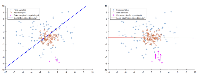
Plot of the Sigmoid Decision Boundary vs. the Least Squared Decision Boundary for Updating the Generator.
Taken from: Least Squares Generative Adversarial Networks.
In addition to avoiding loss saturation, the LSGAN also results in a more stable training process and the generation of higher quality and larger images than the traditional deep convolutional GAN.
First, LSGANs are able to generate higher quality images than regular GANs. Second, LSGANs perform more stable during the learning process.
— Least Squares Generative Adversarial Networks, 2016.
The LSGAN can be implemented by using the target values of 1.0 for real and 0.0 for fake images and optimizing the model using the mean squared error (MSE) loss function, e.g. L2 loss. The output layer of the discriminator model must be a linear activation function.
The authors propose a generator and discriminator model architecture, inspired by the VGG model architecture, and use interleaving upsampling and normal convolutional layers in the generator model, seen on the left in the image below.
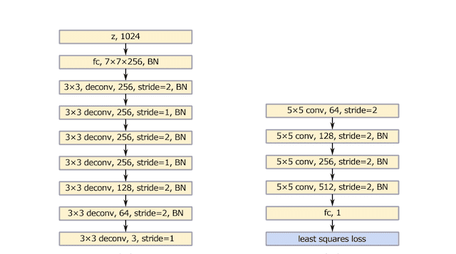
Summary of the Generator (left) and Discriminator (right) Model Architectures used in LSGAN Experiments.
Taken from: Least Squares Generative Adversarial Networks.
Want to Develop GANs from Scratch?
Take my free 7-day email crash course now (with sample code).
Click to sign-up and also get a free PDF Ebook version of the course.
How to Develop an LSGAN for MNIST Handwritten Digits
In this section, we will develop an LSGAN for the MNIST handwritten digit dataset.
The first step is to define the models.
Both the discriminator and the generator will be based on the Deep Convolutional GAN, or DCGAN, architecture. This involves the use of Convolution-BatchNorm-Activation layer blocks with the use of 2×2 stride for downsampling and transpose convolutional layers for upsampling. LeakyReLU activation layers are used in the discriminator and ReLU activation layers are used in the generator.
The discriminator expects grayscale input images with the shape 28×28, the shape of images in the MNIST dataset, and the output layer is a single node with a linear activation function. The model is optimized using the mean squared error (MSE) loss function as per the LSGAN. The define_discriminator() function below defines the discriminator model.
|
1 2 3 4 5 6 7 8 9 10 11 12 13 14 15 16 17 18 19 20 |
# define the standalone discriminator model def define_discriminator(in_shape=(28,28,1)): # weight initialization init = RandomNormal(stddev=0.02) # define model model = Sequential() # downsample to 14x14 model.add(Conv2D(64, (4,4), strides=(2,2), padding='same', kernel_initializer=init, input_shape=in_shape)) model.add(BatchNormalization()) model.add(LeakyReLU(alpha=0.2)) # downsample to 7x7 model.add(Conv2D(128, (4,4), strides=(2,2), padding='same', kernel_initializer=init)) model.add(BatchNormalization()) model.add(LeakyReLU(alpha=0.2)) # classifier model.add(Flatten()) model.add(Dense(1, activation='linear', kernel_initializer=init)) # compile model with L2 loss model.compile(loss='mse', optimizer=Adam(lr=0.0002, beta_1=0.5)) return model |
The generator model takes a point in latent space as input and outputs a grayscale image with the shape 28×28 pixels, where pixel values are in the range [-1,1] via the tanh activation function on the output layer.
The define_generator() function below defines the generator model. This model is not compiled as it is not trained in a standalone manner.
|
1 2 3 4 5 6 7 8 9 10 11 12 13 14 15 16 17 18 19 20 21 22 23 24 |
# define the standalone generator model def define_generator(latent_dim): # weight initialization init = RandomNormal(stddev=0.02) # define model model = Sequential() # foundation for 7x7 image n_nodes = 256 * 7 * 7 model.add(Dense(n_nodes, kernel_initializer=init, input_dim=latent_dim)) model.add(BatchNormalization()) model.add(Activation('relu')) model.add(Reshape((7, 7, 256))) # upsample to 14x14 model.add(Conv2DTranspose(128, (4,4), strides=(2,2), padding='same', kernel_initializer=init)) model.add(BatchNormalization()) model.add(Activation('relu')) # upsample to 28x28 model.add(Conv2DTranspose(64, (4,4), strides=(2,2), padding='same', kernel_initializer=init)) model.add(BatchNormalization()) model.add(Activation('relu')) # output 28x28x1 model.add(Conv2D(1, (7,7), padding='same', kernel_initializer=init)) model.add(Activation('tanh')) return model |
The generator model is updated via the discriminator model. This is achieved by creating a composite model that stacks the generator on top of the discriminator so that error signals can flow back through the discriminator to the generator.
The weights of the discriminator are marked as not trainable when used in this composite model. Updates via the composite model involve using the generator to create new images by providing random points in the latent space as input. The generated images are passed to the discriminator, which will classify them as real or fake. The weights are updated as though the generated images are real (e.g. target of 1.0), allowing the generator to be updated toward generating more realistic images.
The define_gan() function defines and compiles the composite model for updating the generator model via the discriminator, again optimized via mean squared error as per the LSGAN.
|
1 2 3 4 5 6 7 8 9 10 11 12 13 14 15 |
# define the combined generator and discriminator model, for updating the generator def define_gan(generator, discriminator): # make weights in the discriminator not trainable for layer in discriminator.layers: if not isinstance(layer, BatchNormalization): layer.trainable = False # connect them model = Sequential() # add generator model.add(generator) # add the discriminator model.add(discriminator) # compile model with L2 loss model.compile(loss='mse', optimizer=Adam(lr=0.0002, beta_1=0.5)) return model |
Next, we can define a function to load the MNIST handwritten digit dataset and scale the pixel values to the range [-1,1] to match the images output by the generator model.
Only the training part of the MNIST dataset is used, which contains 60,000 centered grayscale images of digits zero through nine.
|
1 2 3 4 5 6 7 8 9 10 11 |
# load mnist images def load_real_samples(): # load dataset (trainX, _), (_, _) = load_data() # expand to 3d, e.g. add channels X = expand_dims(trainX, axis=-1) # convert from ints to floats X = X.astype('float32') # scale from [0,255] to [-1,1] X = (X - 127.5) / 127.5 return X |
We can then define a function to retrieve a batch of randomly selected images from the training dataset.
The real images are returned with corresponding target values for the discriminator model, e.g. y=1.0, to indicate they are real.
|
1 2 3 4 5 6 7 8 9 |
# select real samples def generate_real_samples(dataset, n_samples): # choose random instances ix = randint(0, dataset.shape[0], n_samples) # select images X = dataset[ix] # generate class labels y = ones((n_samples, 1)) return X, y |
Next, we can develop the corresponding functions for the generator.
First, a function for generating random points in the latent space to use as input for generating images via the generator model.
|
1 2 3 4 5 6 7 |
# generate points in latent space as input for the generator def generate_latent_points(latent_dim, n_samples): # generate points in the latent space x_input = randn(latent_dim * n_samples) # reshape into a batch of inputs for the network x_input = x_input.reshape(n_samples, latent_dim) return x_input |
Next, a function that will use the generator model to generate a batch of fake images for updating the discriminator model, along with the target value (y=0) to indicate the images are fake.
|
1 2 3 4 5 6 7 8 9 |
# use the generator to generate n fake examples, with class labels def generate_fake_samples(generator, latent_dim, n_samples): # generate points in latent space x_input = generate_latent_points(latent_dim, n_samples) # predict outputs X = generator.predict(x_input) # create class labels y = zeros((n_samples, 1)) return X, y |
We need to use the generator periodically during training to generate images that we can subjectively inspect and use as the basis for choosing a final generator model.
The summarize_performance() function below can be called during training to generate and save a plot of images and save the generator model. Images are plotted using a reverse grayscale color map to make the digits black on a white background.
|
1 2 3 4 5 6 7 8 9 10 11 12 13 14 15 16 17 18 19 20 21 22 |
# generate samples and save as a plot and save the model def summarize_performance(step, g_model, latent_dim, n_samples=100): # prepare fake examples X, _ = generate_fake_samples(g_model, latent_dim, n_samples) # scale from [-1,1] to [0,1] X = (X + 1) / 2.0 # plot images for i in range(10 * 10): # define subplot pyplot.subplot(10, 10, 1 + i) # turn off axis pyplot.axis('off') # plot raw pixel data pyplot.imshow(X[i, :, :, 0], cmap='gray_r') # save plot to file filename1 = 'generated_plot_%06d.png' % (step+1) pyplot.savefig(filename1) pyplot.close() # save the generator model filename2 = 'model_%06d.h5' % (step+1) g_model.save(filename2) print('Saved %s and %s' % (filename1, filename2)) |
We are also interested in the behavior of loss during training.
As such, we can record loss in lists across each training iteration, then create and save a line plot of the learning dynamics of the models. Creating and saving the plot of learning curves is implemented in the plot_history() function.
|
1 2 3 4 5 6 7 8 9 10 |
# create a line plot of loss for the gan and save to file def plot_history(d1_hist, d2_hist, g_hist): pyplot.plot(d1_hist, label='dloss1') pyplot.plot(d2_hist, label='dloss2') pyplot.plot(g_hist, label='gloss') pyplot.legend() filename = 'plot_line_plot_loss.png' pyplot.savefig(filename) pyplot.close() print('Saved %s' % (filename)) |
Finally, we can define the main training loop via the train() function.
The function takes the defined models and dataset as arguments and parameterizes the number of training epochs and batch size as default function arguments.
Each training loop involves first generating a half-batch of real and fake samples and using them to create one batch worth of weight updates to the discriminator. Next, the generator is updated via the composite model, providing the real (y=1) target as the expected output for the model.
The loss is reported each training iteration, and the model performance is summarized in terms of a plot of generated images at the end of every epoch. The plot of learning curves is created and saved at the end of the run.
|
1 2 3 4 5 6 7 8 9 10 11 12 13 14 15 16 17 18 19 20 21 22 23 24 25 26 27 28 29 30 31 32 33 |
# train the generator and discriminator def train(g_model, d_model, gan_model, dataset, latent_dim, n_epochs=20, n_batch=64): # calculate the number of batches per training epoch bat_per_epo = int(dataset.shape[0] / n_batch) # calculate the number of training iterations n_steps = bat_per_epo * n_epochs # calculate the size of half a batch of samples half_batch = int(n_batch / 2) # lists for storing loss, for plotting later d1_hist, d2_hist, g_hist = list(), list(), list() # manually enumerate epochs for i in range(n_steps): # prepare real and fake samples X_real, y_real = generate_real_samples(dataset, half_batch) X_fake, y_fake = generate_fake_samples(g_model, latent_dim, half_batch) # update discriminator model d_loss1 = d_model.train_on_batch(X_real, y_real) d_loss2 = d_model.train_on_batch(X_fake, y_fake) # update the generator via the discriminator's error z_input = generate_latent_points(latent_dim, n_batch) y_real2 = ones((n_batch, 1)) g_loss = gan_model.train_on_batch(z_input, y_real2) # summarize loss on this batch print('>%d, d1=%.3f, d2=%.3f g=%.3f' % (i+1, d_loss1, d_loss2, g_loss)) # record history d1_hist.append(d_loss1) d2_hist.append(d_loss2) g_hist.append(g_loss) # evaluate the model performance every 'epoch' if (i+1) % (bat_per_epo * 1) == 0: summarize_performance(i, g_model, latent_dim) # create line plot of training history plot_history(d1_hist, d2_hist, g_hist) |
Tying all of this together, the complete code example of training an LSGAN on the MNIST handwritten digit dataset is listed below.
|
1 2 3 4 5 6 7 8 9 10 11 12 13 14 15 16 17 18 19 20 21 22 23 24 25 26 27 28 29 30 31 32 33 34 35 36 37 38 39 40 41 42 43 44 45 46 47 48 49 50 51 52 53 54 55 56 57 58 59 60 61 62 63 64 65 66 67 68 69 70 71 72 73 74 75 76 77 78 79 80 81 82 83 84 85 86 87 88 89 90 91 92 93 94 95 96 97 98 99 100 101 102 103 104 105 106 107 108 109 110 111 112 113 114 115 116 117 118 119 120 121 122 123 124 125 126 127 128 129 130 131 132 133 134 135 136 137 138 139 140 141 142 143 144 145 146 147 148 149 150 151 152 153 154 155 156 157 158 159 160 161 162 163 164 165 166 167 168 169 170 171 172 173 174 175 176 177 178 179 180 181 182 183 184 185 186 187 188 189 190 191 192 193 194 195 196 197 198 199 200 201 202 203 |
# example of lsgan for mnist from numpy import expand_dims from numpy import zeros from numpy import ones from numpy.random import randn from numpy.random import randint from keras.datasets.mnist import load_data from keras.optimizers import Adam from keras.models import Sequential from keras.layers import Dense from keras.layers import Reshape from keras.layers import Flatten from keras.layers import Conv2D from keras.layers import Conv2DTranspose from keras.layers import Activation from keras.layers import LeakyReLU from keras.layers import BatchNormalization from keras.initializers import RandomNormal from matplotlib import pyplot # define the standalone discriminator model def define_discriminator(in_shape=(28,28,1)): # weight initialization init = RandomNormal(stddev=0.02) # define model model = Sequential() # downsample to 14x14 model.add(Conv2D(64, (4,4), strides=(2,2), padding='same', kernel_initializer=init, input_shape=in_shape)) model.add(BatchNormalization()) model.add(LeakyReLU(alpha=0.2)) # downsample to 7x7 model.add(Conv2D(128, (4,4), strides=(2,2), padding='same', kernel_initializer=init)) model.add(BatchNormalization()) model.add(LeakyReLU(alpha=0.2)) # classifier model.add(Flatten()) model.add(Dense(1, activation='linear', kernel_initializer=init)) # compile model with L2 loss model.compile(loss='mse', optimizer=Adam(lr=0.0002, beta_1=0.5)) return model # define the standalone generator model def define_generator(latent_dim): # weight initialization init = RandomNormal(stddev=0.02) # define model model = Sequential() # foundation for 7x7 image n_nodes = 256 * 7 * 7 model.add(Dense(n_nodes, kernel_initializer=init, input_dim=latent_dim)) model.add(BatchNormalization()) model.add(Activation('relu')) model.add(Reshape((7, 7, 256))) # upsample to 14x14 model.add(Conv2DTranspose(128, (4,4), strides=(2,2), padding='same', kernel_initializer=init)) model.add(BatchNormalization()) model.add(Activation('relu')) # upsample to 28x28 model.add(Conv2DTranspose(64, (4,4), strides=(2,2), padding='same', kernel_initializer=init)) model.add(BatchNormalization()) model.add(Activation('relu')) # output 28x28x1 model.add(Conv2D(1, (7,7), padding='same', kernel_initializer=init)) model.add(Activation('tanh')) return model # define the combined generator and discriminator model, for updating the generator def define_gan(generator, discriminator): # make weights in the discriminator not trainable for layer in discriminator.layers: if not isinstance(layer, BatchNormalization): layer.trainable = False # connect them model = Sequential() # add generator model.add(generator) # add the discriminator model.add(discriminator) # compile model with L2 loss model.compile(loss='mse', optimizer=Adam(lr=0.0002, beta_1=0.5)) return model # load mnist images def load_real_samples(): # load dataset (trainX, _), (_, _) = load_data() # expand to 3d, e.g. add channels X = expand_dims(trainX, axis=-1) # convert from ints to floats X = X.astype('float32') # scale from [0,255] to [-1,1] X = (X - 127.5) / 127.5 return X # # select real samples def generate_real_samples(dataset, n_samples): # choose random instances ix = randint(0, dataset.shape[0], n_samples) # select images X = dataset[ix] # generate class labels y = ones((n_samples, 1)) return X, y # generate points in latent space as input for the generator def generate_latent_points(latent_dim, n_samples): # generate points in the latent space x_input = randn(latent_dim * n_samples) # reshape into a batch of inputs for the network x_input = x_input.reshape(n_samples, latent_dim) return x_input # use the generator to generate n fake examples, with class labels def generate_fake_samples(generator, latent_dim, n_samples): # generate points in latent space x_input = generate_latent_points(latent_dim, n_samples) # predict outputs X = generator.predict(x_input) # create class labels y = zeros((n_samples, 1)) return X, y # generate samples and save as a plot and save the model def summarize_performance(step, g_model, latent_dim, n_samples=100): # prepare fake examples X, _ = generate_fake_samples(g_model, latent_dim, n_samples) # scale from [-1,1] to [0,1] X = (X + 1) / 2.0 # plot images for i in range(10 * 10): # define subplot pyplot.subplot(10, 10, 1 + i) # turn off axis pyplot.axis('off') # plot raw pixel data pyplot.imshow(X[i, :, :, 0], cmap='gray_r') # save plot to file filename1 = 'generated_plot_%06d.png' % (step+1) pyplot.savefig(filename1) pyplot.close() # save the generator model filename2 = 'model_%06d.h5' % (step+1) g_model.save(filename2) print('Saved %s and %s' % (filename1, filename2)) # create a line plot of loss for the gan and save to file def plot_history(d1_hist, d2_hist, g_hist): pyplot.plot(d1_hist, label='dloss1') pyplot.plot(d2_hist, label='dloss2') pyplot.plot(g_hist, label='gloss') pyplot.legend() filename = 'plot_line_plot_loss.png' pyplot.savefig(filename) pyplot.close() print('Saved %s' % (filename)) # train the generator and discriminator def train(g_model, d_model, gan_model, dataset, latent_dim, n_epochs=20, n_batch=64): # calculate the number of batches per training epoch bat_per_epo = int(dataset.shape[0] / n_batch) # calculate the number of training iterations n_steps = bat_per_epo * n_epochs # calculate the size of half a batch of samples half_batch = int(n_batch / 2) # lists for storing loss, for plotting later d1_hist, d2_hist, g_hist = list(), list(), list() # manually enumerate epochs for i in range(n_steps): # prepare real and fake samples X_real, y_real = generate_real_samples(dataset, half_batch) X_fake, y_fake = generate_fake_samples(g_model, latent_dim, half_batch) # update discriminator model d_loss1 = d_model.train_on_batch(X_real, y_real) d_loss2 = d_model.train_on_batch(X_fake, y_fake) # update the generator via the discriminator's error z_input = generate_latent_points(latent_dim, n_batch) y_real2 = ones((n_batch, 1)) g_loss = gan_model.train_on_batch(z_input, y_real2) # summarize loss on this batch print('>%d, d1=%.3f, d2=%.3f g=%.3f' % (i+1, d_loss1, d_loss2, g_loss)) # record history d1_hist.append(d_loss1) d2_hist.append(d_loss2) g_hist.append(g_loss) # evaluate the model performance every 'epoch' if (i+1) % (bat_per_epo * 1) == 0: summarize_performance(i, g_model, latent_dim) # create line plot of training history plot_history(d1_hist, d2_hist, g_hist) # size of the latent space latent_dim = 100 # create the discriminator discriminator = define_discriminator() # create the generator generator = define_generator(latent_dim) # create the gan gan_model = define_gan(generator, discriminator) # load image data dataset = load_real_samples() print(dataset.shape) # train model train(generator, discriminator, gan_model, dataset, latent_dim) |
Note: the example can be run on the CPU, although it may take a while and running on GPU hardware is recommended.
Note: Your results may vary given the stochastic nature of the algorithm or evaluation procedure, or differences in numerical precision. Consider running the example a few times and compare the average outcome.
Running the example will report the loss of the discriminator on real (d1) and fake (d2) examples and the loss of the generator via the discriminator on generated examples presented as real (g).
These scores are printed at the end of each training run and are expected to remain small values throughout the training process. Values of zero for an extended period may indicate a failure mode and the training process should be restarted.
|
1 2 3 4 5 6 |
>1, d1=9.292, d2=0.153 g=2.530 >2, d1=1.173, d2=2.057 g=0.903 >3, d1=1.347, d2=1.922 g=2.215 >4, d1=0.604, d2=0.545 g=1.846 >5, d1=0.643, d2=0.734 g=1.619 ... |
Plots of generated images are created at the end of every epoch.
The generated images at the beginning of the run are rough.
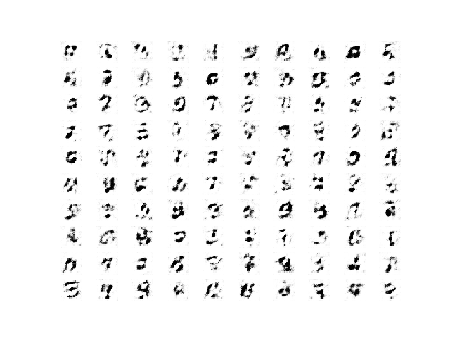
Example of 100 LSGAN Generated Handwritten Digits after 1 Training Epoch
After a handful of training epochs, the generated images begin to look crisp and realistic.
Remember: more training epochs may or may not correspond to a generator that outputs higher quality images. Review the generated plots and choose a final model with the best quality images.
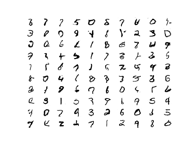
Example of 100 LSGAN Generated Handwritten Digits After 20 Training Epochs
At the end of the training run, a plot of learning curves is created for the discriminator and generator.
In this case, we can see that training remains somewhat stable throughout the run, with some very large peaks observed, which wash out the scale of the plot.
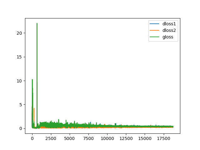
Plot of Learning Curves for the Generator and Discriminator in the LSGAN During Training.
How to Generate Images With LSGAN
We can use the saved generator model to create new images on demand.
This can be achieved by first selecting a final model based on image quality, then loading it and providing new points from the latent space as input in order to generate new plausible images from the domain.
In this case, we will use the model saved after 20 epochs, or 18,740 (60K/64 or 937 batches per epoch * 20 epochs) training iterations.
|
1 2 3 4 5 6 7 8 9 10 11 12 13 14 15 16 17 18 19 20 21 22 23 24 25 26 27 28 29 30 31 32 33 |
# example of loading the generator model and generating images from keras.models import load_model from numpy.random import randn from matplotlib import pyplot # generate points in latent space as input for the generator def generate_latent_points(latent_dim, n_samples): # generate points in the latent space x_input = randn(latent_dim * n_samples) # reshape into a batch of inputs for the network x_input = x_input.reshape(n_samples, latent_dim) return x_input # create a plot of generated images (reversed grayscale) def plot_generated(examples, n): # plot images for i in range(n * n): # define subplot pyplot.subplot(n, n, 1 + i) # turn off axis pyplot.axis('off') # plot raw pixel data pyplot.imshow(examples[i, :, :, 0], cmap='gray_r') pyplot.show() # load model model = load_model('model_018740.h5') # generate images latent_points = generate_latent_points(100, 100) # generate images X = model.predict(latent_points) # plot the result plot_generated(X, 10) |
Running the example generates a plot of 10×10, or 100, new and plausible handwritten digits.
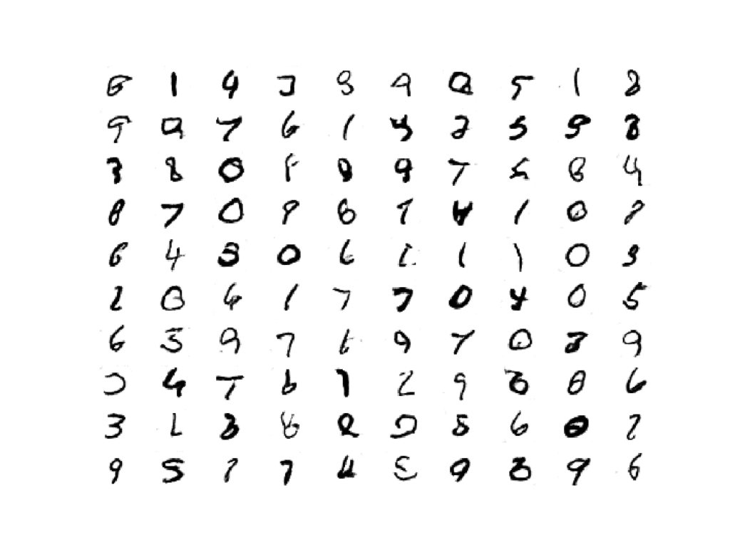
Plot of 100 LSGAN Generated Plausible Handwritten Digits
Further Reading
This section provides more resources on the topic if you are looking to go deeper.
Papers
API
- Keras Datasets API.
- Keras Sequential Model API
- Keras Convolutional Layers API
- How can I “freeze” Keras layers?
- MatplotLib API
- NumPy Random sampling (numpy.random) API
- NumPy Array manipulation routines
Articles
Summary
In this tutorial, you discovered how to develop a least squares generative adversarial network.
Specifically, you learned:
- The LSGAN addresses vanishing gradients and loss saturation of the deep convolutional GAN.
- The LSGAN can be implemented by a mean squared error or L2 loss function for the discriminator model.
- How to implement the LSGAN model for generating handwritten digits for the MNIST dataset.
Do you have any questions?
Ask your questions in the comments below and I will do my best to answer.
Develop Generative Adversarial Networks Today!
Develop Your GAN Models in Minutes
...with just a few lines of python codeDiscover how in my new Ebook:
Generative Adversarial Networks with Python
It provides self-study tutorials and end-to-end projects on:
DCGAN, conditional GANs, image translation, Pix2Pix, CycleGAN
and much more...

 From Scratch")


First of allow me to say you thanks for doing such effort new learner in the field of DL and CV. I have learned a lot of things in the field of Deep learning(DL) and computer vision(CV) form this website. Please, Sir, post a topic related to video super-resolution or automatic video enhancement that how we can do automatic video enhancement. or if you know any website which covers these things with code using GEN or other deep learning methods Then please share with us.
Thanks!
Sorry, I don’t have an example of super resolution at this stage. Perhaps in the future.
Hi Jason,
currently, I am trying to design a “Generative adversarial network” to map a simulation model of a system as a neural network to test if a better execution time can be achieved with similar accuracy.
The simulation model receives real-valued measurement data of its environment and generates a real-valued output from it.
The real-valued measurement data of the environment are limited, so I considered using a Generative Adversarial Network for training the Predictor.
The goal would be for the Generator to generate realistic inputs. These would then be fed into the simulation model to generate the output. Input and output would then be used to train the Predictor.
The overall goal is to get a Predictor with a high quality and a good generalization ability.
The goal of the Generator would be on the one hand to generate inputs as realistic as possible, but on the other hand also to generate inputs for which the Predictor is not yet so well-trained.
What would be the best way to do that?
Perhaps test alternate generative models, e.g. a gaussian process to model the density of the data:
https://machinelearningmastery.com/probability-density-estimation/
For tensorflow 2.0+, please replace keras with tensorflow.keras in the import
Thanks for the suggestion.
The example uses standalone Keras.
Hi,
Is there a particular reason why the last layer in the discriminator has a linear activation? Since we are calculating MSE for values between 0 and 1, doesn’t it make more sense to use a sigmoid instead?
Joshua
Yes, we use a linear output by design to match the MSE loss. Perhaps check the linked paper for more depth.
Thank you for the nice explanation.
I tried the same code in google colab without single modification. I am getting garbage images from the generator and also the loss of both discriminator and generator has gone to 0.
I do not know where the model is going wrong. Can you help?
Perhaps try running it on your workstation or on an AWS EC2 instance instead.
Hello Jason.
Thank you very much for the post, really appreciated it.
I used the code you provided without doing any modifications. I run in Spyder (Python 3.8.3).
However, my results are nowhere close to what you show us. After 20 epochs my results are worse than your 1 epoch results. Do you have any suggestions to why my results are so bad, when using the same code as you?
BR, Aria
Perhaps these tips will help:
https://machinelearningmastery.com/faq/single-faq/why-does-the-code-in-the-tutorial-not-work-for-me
Hello Jason,
First, many thanks for the extensive tutorials, they are very useful!
I have a question regarding the difference in DCGAN and LSGAN training in your tutorials:
DCGAN: real and fake are stacked then train_on_batch() is called on stack
LSGAN: real and fake train_on_batch() is called separately
What is the reason behind this difference?
Given the nature of the training algorithm and loss functions of the models, I would not expect this difference.
Any advice is greatly appreciated.
Many thanks & best regards
Stefano
Sometimes is is good to stack the examples in a batch and sometimes it is good to keep them separate.
It can depend on the dataset and model type. I recommend trying both approaches and discovering what works well or best in your case.
is it similaire to noise loss or not?
sorry, I don’t understand your question. Perhaps you could elaborate or rephrase it?
Hi Jason,
I tried the above approach but it gave really bad results at the end of the training. The discriminator loss quickly saturates to zero and so it seemed like it was the case of convergence failure.
When I added metrics = [“accuracy”] while compiling the discriminator, it worked. But I am unsure as to how adding this resolved the issue.
Hi Saksham…ou may be working on a regression problem and achieve zero prediction errors.
Alternately, you may be working on a classification problem and achieve 100% accuracy.
This is unusual and there are many possible reasons for this, including:
You are evaluating model performance on the training set by accident.
Your hold out dataset (train or validation) is too small or unrepresentative.
You have introduced a bug into your code and it is doing something different from what you expect.
Your prediction problem is easy or trivial and may not require machine learning.
The most common reason is that your hold out dataset is too small or not representative of the broader problem.
This can be addressed by:
Using k-fold cross-validation to estimate model performance instead of a train/test split.
Gather more data.
Use a different split of data for train and test, such as 50/50.
Hi Jason,
Thank you so much for showing many DL implementation codes on this site.
Is it possible for you to show how to implement energy-based GAN (EBGAN) and boundary equilibrium GAN (BEGAN) with Keras? I am confused with the loss functions of these GANs, should these GANs use Lambda layers for customized loss function definitions?
Hi Hsiao…The following is a great starting point for working with GANs:
https://machinelearningmastery.com/resources-for-getting-started-with-generative-adversarial-networks/