Probability density is the relationship between observations and their probability.
Some outcomes of a random variable will have low probability density and other outcomes will have a high probability density.
The overall shape of the probability density is referred to as a probability distribution, and the calculation of probabilities for specific outcomes of a random variable is performed by a probability density function, or PDF for short.
It is useful to know the probability density function for a sample of data in order to know whether a given observation is unlikely, or so unlikely as to be considered an outlier or anomaly and whether it should be removed. It is also helpful in order to choose appropriate learning methods that require input data to have a specific probability distribution.
It is unlikely that the probability density function for a random sample of data is known. As such, the probability density must be approximated using a process known as probability density estimation.
In this tutorial, you will discover a gentle introduction to probability density estimation.
After completing this tutorial, you will know:
- Histogram plots provide a fast and reliable way to visualize the probability density of a data sample.
- Parametric probability density estimation involves selecting a common distribution and estimating the parameters for the density function from a data sample.
- Nonparametric probability density estimation involves using a technique to fit a model to the arbitrary distribution of the data, like kernel density estimation.
Kick-start your project with my new book Probability for Machine Learning, including step-by-step tutorials and the Python source code files for all examples.
Let’s get started.

A Gentle Introduction to Probability Density Estimation
Photo by Alistair Paterson, some rights reserved.
Tutorial Overview
This tutorial is divided into four parts; they are:
- Probability Density
- Summarize Density With a Histogram
- Parametric Density Estimation
- Nonparametric Density Estimation
Probability Density
A random variable x has a probability distribution p(x).
The relationship between the outcomes of a random variable and its probability is referred to as the probability density, or simply the “density.”
If a random variable is continuous, then the probability can be calculated via probability density function, or PDF for short. The shape of the probability density function across the domain for a random variable is referred to as the probability distribution and common probability distributions have names, such as uniform, normal, exponential, and so on.
Given a random variable, we are interested in the density of its probabilities.
For example, given a random sample of a variable, we might want to know things like the shape of the probability distribution, the most likely value, the spread of values, and other properties.
Knowing the probability distribution for a random variable can help to calculate moments of the distribution, like the mean and variance, but can also be useful for other more general considerations, like determining whether an observation is unlikely or very unlikely and might be an outlier or anomaly.
The problem is, we may not know the probability distribution for a random variable. We rarely do know the distribution because we don’t have access to all possible outcomes for a random variable. In fact, all we have access to is a sample of observations. As such, we must select a probability distribution.
This problem is referred to as probability density estimation, or simply “density estimation,” as we are using the observations in a random sample to estimate the general density of probabilities beyond just the sample of data we have available.
There are a few steps in the process of density estimation for a random variable.
The first step is to review the density of observations in the random sample with a simple histogram. From the histogram, we might be able to identify a common and well-understood probability distribution that can be used, such as a normal distribution. If not, we may have to fit a model to estimate the distribution.
In the following sections, we will take a closer look at each one of these steps in turn.
We will focus on univariate data, e.g. one random variable, in this post for simplicity. Although the steps are applicable for multivariate data, they can become more challenging as the number of variables increases.
Want to Learn Probability for Machine Learning
Take my free 7-day email crash course now (with sample code).
Click to sign-up and also get a free PDF Ebook version of the course.
Summarize Density With a Histogram
The first step in density estimation is to create a histogram of the observations in the random sample.
A histogram is a plot that involves first grouping the observations into bins and counting the number of events that fall into each bin. The counts, or frequencies of observations, in each bin are then plotted as a bar graph with the bins on the x-axis and the frequency on the y-axis.
The choice of the number of bins is important as it controls the coarseness of the distribution (number of bars) and, in turn, how well the density of the observations is plotted. It is a good idea to experiment with different bin sizes for a given data sample to get multiple perspectives or views on the same data.
For example, observations between 1 and 100 could be split into 3 bins (1-33, 34-66, 67-100), which might be too coarse, or 10 bins (1-10, 11-20, … 91-100), which might better capture the density.
A histogram can be created using the Matplotlib library and the hist() function. The data is provided as the first argument, and the number of bins is specified via the “bins” argument either as an integer (e.g. 10) or as a sequence of the boundaries of each bin (e.g. [1, 34, 67, 100]).
The snippet below creates a histogram with 10 bins for a data sample.
|
1 2 3 4 |
... # plot a histogram of the sample pyplot.hist(sample, bins=10) pyplot.show() |
We can create a random sample drawn from a normal distribution and pretend we don’t know the distribution, then create a histogram of the data. The normal() NumPy function will achieve this and we will generate 1,000 samples with a mean of 0 and a standard deviation of 1, e.g. a standard Gaussian.
The complete example is listed below.
|
1 2 3 4 5 6 7 8 |
# example of plotting a histogram of a random sample from matplotlib import pyplot from numpy.random import normal # generate a sample sample = normal(size=1000) # plot a histogram of the sample pyplot.hist(sample, bins=10) pyplot.show() |
Running the example draws a sample of random observations and creates the histogram with 10 bins. We can clearly see the shape of the normal distribution.
Note that your results will differ given the random nature of the data sample. Try running the example a few times.
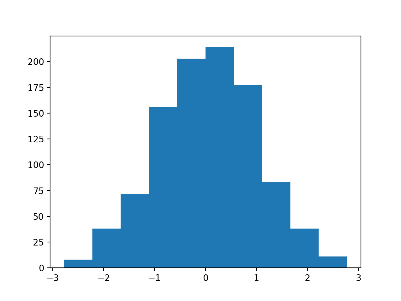
Histogram Plot With 10 Bins of a Random Data Sample
Running the example with bins set to 3 makes the normal distribution less obvious.
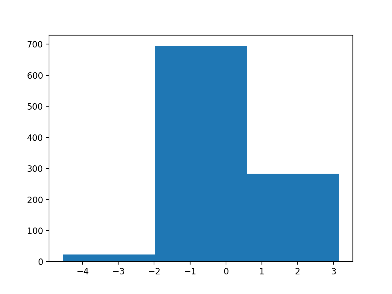
Histogram Plot With 3 Bins of a Random Data Sample
Reviewing a histogram of a data sample with a range of different numbers of bins will help to identify whether the density looks like a common probability distribution or not.
In most cases, you will see a unimodal distribution, such as the familiar bell shape of the normal, the flat shape of the uniform, or the descending or ascending shape of an exponential or Pareto distribution.
You might also see complex distributions, such as multiple peaks that don’t disappear with different numbers of bins, referred to as a bimodal distribution, or multiple peaks, referred to as a multimodal distribution. You might also see a large spike in density for a given value or small range of values indicating outliers, often occurring on the tail of a distribution far away from the rest of the density.
Parametric Density Estimation
The shape of a histogram of most random samples will match a well-known probability distribution.
The common distributions are common because they occur again and again in different and sometimes unexpected domains.
Get familiar with the common probability distributions as it will help you to identify a given distribution from a histogram.
Once identified, you can attempt to estimate the density of the random variable with a chosen probability distribution. This can be achieved by estimating the parameters of the distribution from a random sample of data.
For example, the normal distribution has two parameters: the mean and the standard deviation. Given these two parameters, we now know the probability distribution function. These parameters can be estimated from data by calculating the sample mean and sample standard deviation.
We refer to this process as parametric density estimation.
The reason is that we are using predefined functions to summarize the relationship between observations and their probability that can be controlled or configured with parameters, hence “parametric“.
Once we have estimated the density, we can check if it is a good fit. This can be done in many ways, such as:
- Plotting the density function and comparing the shape to the histogram.
- Sampling the density function and comparing the generated sample to the real sample.
- Using a statistical test to confirm the data fits the distribution.
We can demonstrate this with an example.
We can generate a random sample of 1,000 observations from a normal distribution with a mean of 50 and a standard deviation of 5.
|
1 2 3 |
... # generate a sample sample = normal(loc=50, scale=5, size=1000) |
We can then pretend that we don’t know the probability distribution and maybe look at a histogram and guess that it is normal. Assuming that it is normal, we can then calculate the parameters of the distribution, specifically the mean and standard deviation.
We would not expect the mean and standard deviation to be 50 and 5 exactly given the small sample size and noise in the sampling process.
|
1 2 3 4 5 |
... # calculate parameters sample_mean = mean(sample) sample_std = std(sample) print('Mean=%.3f, Standard Deviation=%.3f' % (sample_mean, sample_std)) |
Then fit the distribution with these parameters, so-called parametric density estimation of our data sample.
In this case, we can use the norm() SciPy function.
|
1 2 3 |
... # define the distribution dist = norm(sample_mean, sample_std) |
We can then sample the probabilities from this distribution for a range of values in our domain, in this case between 30 and 70.
|
1 2 3 4 |
... # sample probabilities for a range of outcomes values = [value for value in range(30, 70)] probabilities = [dist.pdf(value) for value in values] |
Finally, we can plot a histogram of the data sample and overlay a line plot of the probabilities calculated for the range of values from the PDF.
Importantly, we can convert the counts or frequencies in each bin of the histogram to a normalized probability to ensure the y-axis of the histogram matches the y-axis of the line plot. This can be achieved by setting the “density” argument to “True” in the call to hist().
|
1 2 3 4 |
... # plot the histogram and pdf pyplot.hist(sample, bins=10, density=True) pyplot.plot(values, probabilities) |
Tying these snippets together, the complete example of parametric density estimation is listed below.
|
1 2 3 4 5 6 7 8 9 10 11 12 13 14 15 16 17 18 19 20 21 |
# example of parametric probability density estimation from matplotlib import pyplot from numpy.random import normal from numpy import mean from numpy import std from scipy.stats import norm # generate a sample sample = normal(loc=50, scale=5, size=1000) # calculate parameters sample_mean = mean(sample) sample_std = std(sample) print('Mean=%.3f, Standard Deviation=%.3f' % (sample_mean, sample_std)) # define the distribution dist = norm(sample_mean, sample_std) # sample probabilities for a range of outcomes values = [value for value in range(30, 70)] probabilities = [dist.pdf(value) for value in values] # plot the histogram and pdf pyplot.hist(sample, bins=10, density=True) pyplot.plot(values, probabilities) pyplot.show() |
Running the example first generates the data sample, then estimates the parameters of the normal probability distribution.
Note that your results will differ given the random nature of the data sample. Try running the example a few times.
In this case, we can see that the mean and standard deviation have some noise and are slightly different from the expected values of 50 and 5 respectively. The noise is minor and the distribution is expected to still be a good fit.
|
1 |
Mean=49.852, Standard Deviation=5.023 |
Next, the PDF is fit using the estimated parameters and the histogram of the data with 10 bins is compared to probabilities for a range of values sampled from the PDF.
We can see that the PDF is a good match for our data.
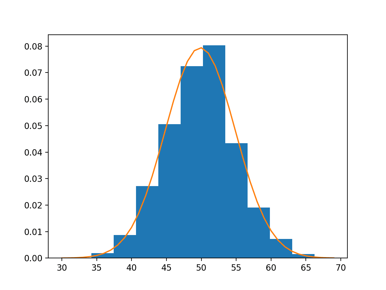
Data Sample Histogram With Probability Density Function Overlay for the Normal Distribution
It is possible that the data does match a common probability distribution, but requires a transformation before parametric density estimation.
For example, you may have outlier values that are far from the mean or center of mass of the distribution. This may have the effect of giving incorrect estimates of the distribution parameters and, in turn, causing a poor fit to the data. These outliers should be removed prior to estimating the distribution parameters.
Another example is the data may have a skew or be shifted left or right. In this case, you might need to transform the data prior to estimating the parameters, such as taking the log or square root, or more generally, using a power transform like the Box-Cox transform.
These types of modifications to the data may not be obvious and effective parametric density estimation may require an iterative process of:
- Loop Until Fit of Distribution to Data is Good Enough:
- 1. Estimating distribution parameters
- 2. Reviewing the resulting PDF against the data
- 3. Transforming the data to better fit the distribution
Nonparametric Density Estimation
In some cases, a data sample may not resemble a common probability distribution or cannot be easily made to fit the distribution.
This is often the case when the data has two peaks (bimodal distribution) or many peaks (multimodal distribution).
In this case, parametric density estimation is not feasible and alternative methods can be used that do not use a common distribution. Instead, an algorithm is used to approximate the probability distribution of the data without a pre-defined distribution, referred to as a nonparametric method.
The distributions will still have parameters but are not directly controllable in the same way as simple probability distributions. For example, a nonparametric method might estimate the density using all observations in a random sample, in effect making all observations in the sample “parameters.”
Perhaps the most common nonparametric approach for estimating the probability density function of a continuous random variable is called kernel smoothing, or kernel density estimation, KDE for short.
- Kernel Density Estimation: Nonparametric method for using a dataset to estimating probabilities for new points.
In this case, a kernel is a mathematical function that returns a probability for a given value of a random variable. The kernel effectively smooths or interpolates the probabilities across the range of outcomes for a random variable such that the sum of probabilities equals one, a requirement of well-behaved probabilities.
The kernel function weights the contribution of observations from a data sample based on their relationship or distance to a given query sample for which the probability is requested.
A parameter, called the smoothing parameter or the bandwidth, controls the scope, or window of observations, from the data sample that contributes to estimating the probability for a given sample. As such, kernel density estimation is sometimes referred to as a Parzen-Rosenblatt window, or simply a Parzen window, after the developers of the method.
- Smoothing Parameter (bandwidth): Parameter that controls the number of samples or window of samples used to estimate the probability for a new point.
A large window may result in a coarse density with little details, whereas a small window may have too much detail and not be smooth or general enough to correctly cover new or unseen examples. The contribution of samples within the window can be shaped using different functions, sometimes referred to as basis functions, e.g. uniform normal, etc., with different effects on the smoothness of the resulting density function.
- Basis Function (kernel): The function chosen used to control the contribution of samples in the dataset toward estimating the probability of a new point.
As such, it may be useful to experiment with different window sizes and different contribution functions and evaluate the results against histograms of the data.
We can demonstrate this with an example.
First, we can construct a bimodal distribution by combining samples from two different normal distributions. Specifically, 300 examples with a mean of 20 and a standard deviation of 5 (the smaller peak), and 700 examples with a mean of 40 and a standard deviation of 5 (the larger peak). The means were chosen close together to ensure the distributions overlap in the combined sample.
The complete example of creating this sample with a bimodal probability distribution and plotting the histogram is listed below.
|
1 2 3 4 5 6 7 8 9 10 11 |
# example of a bimodal data sample from matplotlib import pyplot from numpy.random import normal from numpy import hstack # generate a sample sample1 = normal(loc=20, scale=5, size=300) sample2 = normal(loc=40, scale=5, size=700) sample = hstack((sample1, sample2)) # plot the histogram pyplot.hist(sample, bins=50) pyplot.show() |
Running the example creates the data sample and plots the histogram.
Note that your results will differ given the random nature of the data sample. Try running the example a few times.
We have fewer samples with a mean of 20 than samples with a mean of 40, which we can see reflected in the histogram with a larger density of samples around 40 than around 20.
Data with this distribution does not nicely fit into a common probability distribution, by design. It is a good case for using a nonparametric kernel density estimation method.
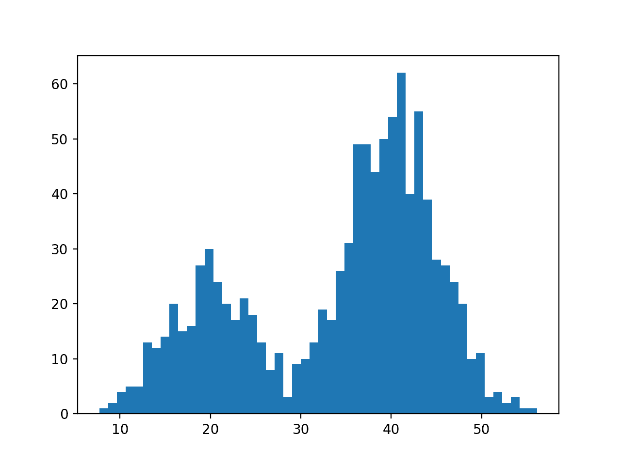
Histogram Plot of Data Sample With a Bimodal Probability Distribution
The scikit-learn machine learning library provides the KernelDensity class that implements kernel density estimation.
First, the class is constructed with the desired bandwidth (window size) and kernel (basis function) arguments. It is a good idea to test different configurations on your data. In this case, we will try a bandwidth of 2 and a Gaussian kernel.
The class is then fit on a data sample via the fit() function. The function expects the data to have a 2D shape with the form [rows, columns], therefore we can reshape our data sample to have 1,000 rows and 1 column.
|
1 2 3 4 5 |
... # fit density model = KernelDensity(bandwidth=2, kernel='gaussian') sample = sample.reshape((len(sample), 1)) model.fit(sample) |
We can then evaluate how well the density estimate matches our data by calculating the probabilities for a range of observations and comparing the shape to the histogram, just like we did for the parametric case in the prior section.
The score_samples() function on the KernelDensity will calculate the log probability for an array of samples. We can create a range of samples from 1 to 60, about the range of our domain, calculate the log probabilities, then invert the log operation by calculating the exponent or exp() to return the values to the range 0-1 for normal probabilities.
|
1 2 3 4 5 6 |
... # sample probabilities for a range of outcomes values = asarray([value for value in range(1, 60)]) values = values.reshape((len(values), 1)) probabilities = model.score_samples(values) probabilities = exp(probabilities) |
Finally, we can create a histogram with normalized frequencies and an overlay line plot of values to estimated probabilities.
|
1 2 3 4 5 |
... # plot the histogram and pdf pyplot.hist(sample, bins=50, density=True) pyplot.plot(values[:], probabilities) pyplot.show() |
Tying this together, the complete example of kernel density estimation for a bimodal data sample is listed below.
|
1 2 3 4 5 6 7 8 9 10 11 12 13 14 15 16 17 18 19 20 21 22 23 24 |
# example of kernel density estimation for a bimodal data sample from matplotlib import pyplot from numpy.random import normal from numpy import hstack from numpy import asarray from numpy import exp from sklearn.neighbors import KernelDensity # generate a sample sample1 = normal(loc=20, scale=5, size=300) sample2 = normal(loc=40, scale=5, size=700) sample = hstack((sample1, sample2)) # fit density model = KernelDensity(bandwidth=2, kernel='gaussian') sample = sample.reshape((len(sample), 1)) model.fit(sample) # sample probabilities for a range of outcomes values = asarray([value for value in range(1, 60)]) values = values.reshape((len(values), 1)) probabilities = model.score_samples(values) probabilities = exp(probabilities) # plot the histogram and pdf pyplot.hist(sample, bins=50, density=True) pyplot.plot(values[:], probabilities) pyplot.show() |
Running the example creates the data distribution, fits the kernel density estimation model, then plots the histogram of the data sample and the PDF from the KDE model.
Note that your results will differ given the random nature of the data sample. Try running the example a few times.
In this case, we can see that the PDF is a good fit for the histogram. It is not very smooth and could be made more so by setting the “bandwidth” argument to 3 samples or higher. Experiment with different values of the bandwidth and the kernel function.
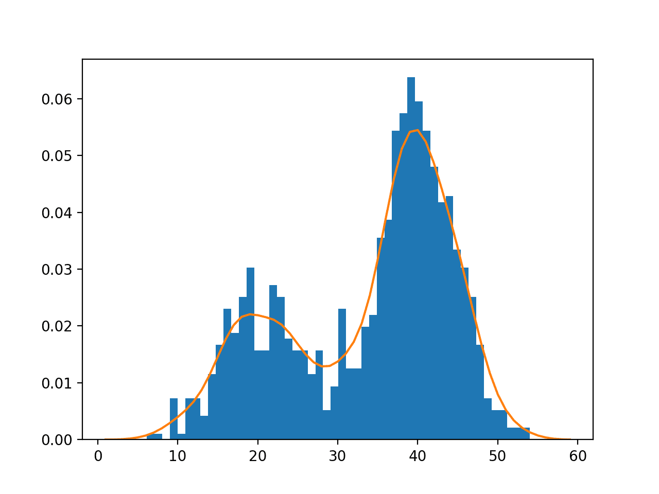
Histogram and Probability Density Function Plot Estimated via Kernel Density Estimation for a Bimodal Data Sample
The KernelDensity class is powerful and does support estimating the PDF for multidimensional data.
Further Reading
This section provides more resources on the topic if you are looking to go deeper.
Books
- Pattern Recognition and Machine Learning, 2006.
- Machine Learning: A Probabilistic Perspective, 2012.
- The Elements of Statistical Learning: Data Mining, Inference, and Prediction, 2009.
API
- scipy.stats.gaussian_kde API.
- Nonparametric Methods nonparametric, Statsmodels API.
- Kernel Density Estimation Statsmodels Example.
- Density Estimation, Scikit-Learn API.
Articles
- Density estimation, Wikipedia.
- Histogram, Wikipedia.
- Kernel density estimation, Wikipedia.
- Multivariate kernel density estimation, Wikipedia.
- Kernel density estimation via the Parzen-Rosenblatt window method, 2014.
- In-Depth: Kernel Density Estimation.
Summary
In this tutorial, you discovered a gentle introduction to probability density estimation.
Specifically, you learned:
- Histogram plots provide a fast and reliable way to visualize the probability density of a data sample.
- Parametric probability density estimation involves selecting a common distribution and estimating the parameters for the density function from a data sample.
- Nonparametric probability density estimation involves using a technique to fit a model to the arbitrary distribution of the data, like kernel density estimation.
Do you have any questions?
Ask your questions in the comments below and I will do my best to answer.
Get a Handle on Probability for Machine Learning!

Develop Your Understanding of Probability
...with just a few lines of python codeDiscover how in my new Ebook:
Probability for Machine Learning
It provides self-study tutorials and end-to-end projects on:
Bayes Theorem, Bayesian Optimization, Distributions, Maximum Likelihood, Cross-Entropy, Calibrating Models
and much more...


Hello and thanks for the useful post! I’d like to ask a question. In parametric estimation, would it be wrong to calculate fist.pdf for the elements of sample list instead of the numbers 30-69? I’m not sure I understand why we need to do it for new values and not for the previously generated sample. Thanks
Sorry, I don’t follow your question.
Can you elaborate please?
Certainly. It was badly expressed for sure, sorry. We generate 1000 numbers from normal distribution with mean 50 and std 5 and we make the histogram of those values. We suppose we dont know this sample originates from a normal distr., and we see from the higstogram that it indeed could come from one. Now we want to actually estimate this actual normal distribution. The best estimators for its 2 parameters, mean and std are the respective mean, std of our previously generated sample.
This where I got a bit lost. We want to “draw” this normal distr together with the histogram, and see if it fits well to it. What confused me, why do we calculate the pdf of this normal distr. for the values 30-69 (range(30,70)) ? Would it be wrong to generate numbers from the normal distribution with mean = sample_mean and std = sample_std and compute the pdf for these values? Or even, calculate the pdf of this normal dist for the previously generated sample? What I mean is that code would be the following
probabilities = [dist.pdf(newsample) for index in newsample], where newsample = normal(mean_sample, mean_std, size = )
or
probabilities = [dist.pdf(sample) for index in sample]
Sorry for the huge question, and thanks for the answer !
No need to generate random numbers, we can just enumerate the domain at some resolution and use the pdf to get the prob for the y-axis of the graph.
Does that help?
Yeah I think I figured it out. We have the data generated from normal (we don’t know that supposedly) and we believe that the distribution that fits into this data is the normal distr with sample_mean and sample_std. In order to test this we create the hist of the data and we sketch the normal distr. I was a bit confused but yeah now I get it !
Regarding the kernel density estimation, the “fit” function basically takes our kernel function and creates the respective estimated pdf, i.e. (1/Nh^d) * sum{ f( (x-xi) / h) } ? Sorry for the not so good expression. Thanks !
Something like that, but on a local level, not across the whole domain.
Also sorry for double post, but do you know if KernelDensity function can take as kernel the uniform distribution? I look at the documentation but i dont think it can and it seems weird !
Yes, it will approximate whatever you have.
Sweet, thanks for the guide once more! Have a good day.
You’re welcome.
thanks you
You’re welcome.
Hello,
Sorry but It seems to have a bug in your guide.
You are only plotting the density calculated by pyplot.hist and not the one you calculated with KernelDensity.
Try with :
pyplot.hist(sample, bins=50, density=False)
You will have not density at all, because the hist data are not in the same scale as the PDF.
T
Thanks for your note, I will investigate.
Update: I believe the examples are correct. Setting density=True ensures the histogram is scaled. The line plot is still drawn over the top of the histogram.
Hello, and thanks for your post!
I want to compare the AIC of a kernel density estimate with that of a parametric model. I can calculate the loglikelihood of the KDE but how do I know how many effective parameters the KDE estimates? Is it necessarily the same as the number of data points? Possibly plus the bandwidth.
Thanks,
F d C
Good question, I recommend checking the literature for KFD specific calculations of AIC rather than deriving your own.
Really nice blog post, as usual, I just applied it to a real case to compare how well each approximation (parametric VS non-parametric) works for my real case with nice results (winning the non-parametric, thanks!
By the way, isn’t it ok to basically apply the non-parametric option, since it does not assume any distribution, being also useful to be applied to parametric ones? That way we should not care about the distribution type.
Thanks!
Yes, but we should use the simplest possible viable method for a given problem.
Actually I was optimistic to get a discussion about what is meant by the probability of the data. We hear this e.g. when discussing generative model. I mean if some one wants to estimate the probability of real images, what that looks like? I know you may say that is complex to visualize, but a 2*2 image will do for me 🙂
thanks
I think you are referring to predicting the probability of a class label.
This would be a probability distribution over all candidate classes conditional on the input data.
Actually my exact question, is if I have e.g. 3*3 images and I want to estimate the probability distribution for that data, to be able to sample new images from it. Then, if I serialize these images to 1-D vectors with 9 elements (features); does that mean I have 9 random variables then I should estimate 9 probability distributions? or may be 1 probability distribution which has 9 dimensions?
Not sure I follow, sorry.
You have 9 images, and you want to sample them, randomly, then that is a uniform probability distribution or a 1/9 probability of any image being selected.
Dear Json,
there is a typo in section “Parametric Density Estimation”. In the first code snippet in this section, the number of sampled points is 1000, but two lines above that, it is mentioned we draw a sample of 100 points.
Where exactly?
Before the first snippet I see:
Before the first snippet in section “Parametric Density Estimation” which is the third code snippet from the beginning.
Look for this:
“We can generate a random sample of 100 observations from a normal distribution with a mean of 50 and a standard deviation of 5.”
Thanks! Fixed.
Dear Jason,
Thanks for the useful post. I would like to know whether I can plot the density of entropies of 300 samples by your tutorial or just I can plot the density of entropy of one sample.
Please let me know as soon as possible, since I need it for a paper Which is under reviewed and a reviewer asked me to plot the density of entropies for all images
Thank you in advance for replying so quickly.
Best
Maryam
Sorry, I don’t know what “density of entropies” means.
Hi,
Thank you for this wonderful tutorial!
I have two questions:
1) How do you output the formula of the PDF after the KDE is done estimating?
2) How do you estimate the joint PDF for 2D data with the KDE?
Many thanks in advance!
You don’t, you have a model that captures the distribution.
Good question, I believe the library supports multivariate distributions. Perhaps try it or check the documentation.
Hi Jason,
Many thanks for your reply.
I have a follow up question. Suppose my PDF is of the form f(x,y) and the 2D histogram is represented as such. Using the KDE, I capture the distribution. Now suppose I am to integrate over f(x,y) (i.e. \int f(x,y) dx). With my distribution, how can I output useful info so I can perform this integration if I do not know the formula of f(x,y)?
Many thanks in advance,
Ameir
One approach might be to use the empirical distribution function:
https://machinelearningmastery.com/empirical-distribution-function-in-python/
Hi,
Question about Parametric Density Estimation: what is the minimal number of samples that goes into 1 bin? For your example 10, 20 and 40 bins (so 100, 50, and 25 samples per bin) seem to fit well with the calculated normal distribution from the sample mean and standard deviation (drawn as a line on top of the histogram). However, if I pick say 80 bins the fit is not that obvious anymore. Is there a recommended minimum number of samples per bin in this case?
I’ve been reading some time ago about the concept of a sample of sample means which says that basically if your sample size is above 30 and you collect multiple such samples then the mean of the samples means approaches the “true mean”. Does it apply here somehow for selecting the number of samples that go into 1 bin?
There may be, I don’t know off the cuff. Perhaps experiment with your data. Or perhaps check some of the reference in the further reading section.
I think you’re referring to the central limit theorem:
https://machinelearningmastery.com/a-gentle-introduction-to-the-central-limit-theorem-for-machine-learning/
Or the law of large numbers:
https://machinelearningmastery.com/a-gentle-introduction-to-the-law-of-large-numbers-in-machine-learning/
Hi Jason,
Is it possible that the Kernel Density estimator gives me a function of the continuous distribution instead of an array of points which is limited to the range of my data? When I want to plot the resulting distribution it is always cut of at the limits of my data, which sometimes results in an ugly plot (instead of decreasing to zero at the boundaries). When my kernel is a continuous gaussian, KDE should provide my with a continuous function.
Yes, KDF gives a continuous function that you can query.
How to find probability density function for dependent /class variable in the dataset?
You can use an empirical distribution for any data:
https://machinelearningmastery.com/empirical-distribution-function-in-python/
Hi Jason,
quesiton about Conditional Probability:For example,I have the PDF P(A丨B),but how to plot this picture like you? Is it choosing a constant value B and plot the histogram?
Perhaps a scatter plot of a sample of the two variables?
Thanx dear Jason Brownlee
It is very useful, and i am interested to generate continuous PDF for real world data sets. Kindly recommend me the books and rsearch papers to work on this side.
Rafiullah assistant professor of Statistics at college level.
Thanks for the article, very informative. Just a note that it was better to use sample.reshape(-1,1) instead of using sample.reshape((len(sample), 1)).
Thanks, I prefer the explicit approach.
I have two vectors with different lengths, and I need to compare their probability density functions. How can I do this? Shall I normalize the two vectors before plotting in order to avoid the problem of the different size of the two vectors?
Vector of different length should not be a problem. You can still plot their density on the same graph using pyplot.hist()
Hello!
It a really well sumamrized introduction to the topic. I really need more information on the parametric estimation part where some of the samples (tail samples) are neglected for better estimation. I have a problem that fits the description. It would be actually helpful if you can refer to a theoritical based reference that have an algorithm or describes how to optimally choose a certain window of the samples to get the best estimation. One intuition will be for example to get the samples closer to the mean value as a function of the variance.
Hello there,
Thank you so much for this. I can say I have a better understanding of density estimation
Thank you for your feedback!
Hi Jason
Thanks for this article. I found it really helpful.
It strikes me that the y-axes of a histogram can represent for each bar representing
a bin:
(1) Frequency: a count of the number of data points in the bin.
(2) Relative frequency: (the number of data points in the bin/total data points) x 100.
(3) Probability: the area of the bar for a bin/total area of histogram.
Is this right, because bins can be of different sizes, so we use the area to assign
probabilities for each bin ?
Absolutey Darshan! Your understanding is correct! Keep up the great work!
Hi Jason,
Thanks for this very informative tutorial and your book about probability is really well explained.
Great feedback Ehtisham!
Dear Dr. Brownlee
thanks for all your useful and smooth explanations.
i have a question in mind, in non-parametric probability estimation the final answer requires a distribution or not?
Hi RHZ…The following may help add clarity:
https://faun.pub/parametric-and-nonparametric-machine-learning-algorithm-6134d7155cc
Do you have an article implementing the algorithms from scratch or some guidance?
Hi george…The following resource may be of interest to you:
https://billc.io/2023/01/kde-from-scratch/