Data transforms are intended to remove noise and improve the signal in time series forecasting.
It can be very difficult to select a good, or even best, transform for a given prediction problem. There are many transforms to choose from and each has a different mathematical intuition.
In this tutorial, you will discover how to explore different power-based transforms for time series forecasting with Python.
After completing this tutorial, you will know:
How to identify when to use and how to explore a square root transform.
How to identify when to use and explore a log transform and the expectations on raw data.
How to use the Box-Cox transform to perform square root, log, and automatically discover the best power transform for your dataset.
Kick-start your project with my new book Time Series Forecasting With Python, including step-by-step tutorials and the Python source code files for all examples.
Let’s get started.
Updated Apr/2019: Updated the link to dataset.
Updated Aug/2019: Updated data loading to use new API.
Airline Passengers Dataset
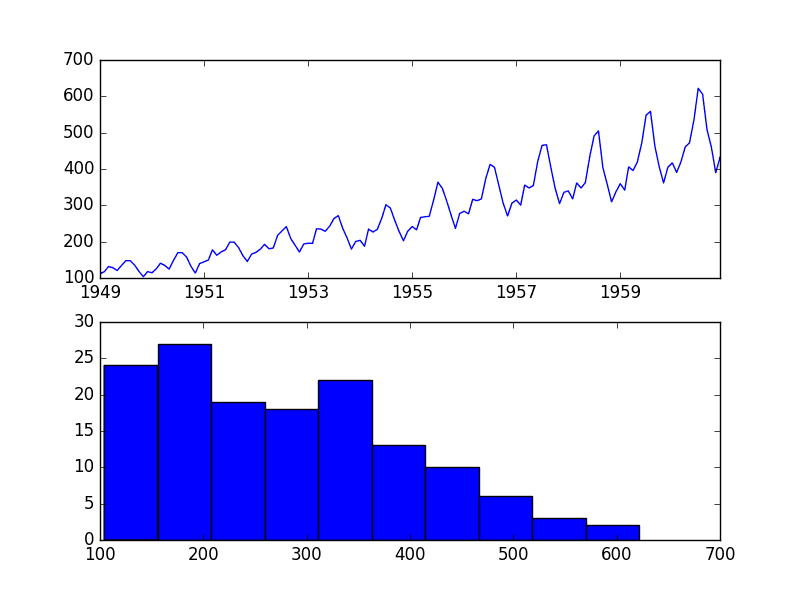
The Airline Passengers dataset describes a total number of airline passengers over time.
The units are a count of the number of airline passengers in thousands. There are 144 monthly observations from 1949 to 1960.
Running the example creates two plots, the first showing the time series as a line plot and the second showing the observations as a histogram.
Airline Passengers Dataset Plot
The dataset is non-stationary, meaning that the mean and the variance of the observations change over time. This makes it difficult to model by both classical statistical methods, like ARIMA, and more sophisticated machine learning methods, like neural networks.
This is caused by what appears to be both an increasing trend and a seasonality component.
In addition, the amount of change, or the variance, is increasing with time. This is clear when you look at the size of the seasonal component and notice that from one cycle to the next, the amplitude (from bottom to top of the cycle) is increasing.
In this tutorial, we will investigate transforms that we can use on time series datasets that exhibit this property.
Stop learning Time Series Forecasting the slow way!
Take my free 7-day email course and discover how to get started (with sample code).
Click to sign-up and also get a free PDF Ebook version of the course.
Square Root Transform
A time series that has a quadratic growth trend can be made linear by taking the square root.
Let’s demonstrate this with a quick contrived example.
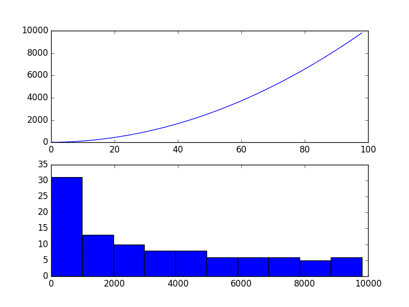
Consider a series of the numbers 1 to 99 squared. The line plot of this series will show a quadratic growth trend and a histogram of the values will show an exponential distribution with a long trail.
The snippet of code below creates and graphs this series.
1
2
3
4
5
6
7
8
from matplotlib import pyplot
series=[i**2foriinrange(1,100)]
# line plot
pyplot.plot(series)
pyplot.show()
# histogram
pyplot.hist(series)
pyplot.show()
Running the example plots the series both as a line plot over time and a histogram of observations.
Quadratic Time Series
If you see a structure like this in your own time series, you may have a quadratic growth trend. This can be removed or made linear by taking the inverse operation of the squaring procedure, which is the square root.
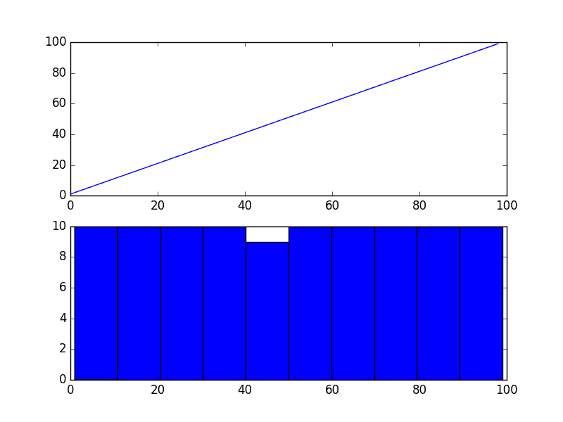
Because the example is perfectly quadratic, we would expect the line plot of the transformed data to show a straight line. Because the source of the squared series is linear, we would expect the histogram to show a uniform distribution.
The example below performs a sqrt() transform on the time series and plots the result.
1
2
3
4
5
6
7
8
9
10
11
12
13
from matplotlib import pyplot
from numpy import sqrt
series=[i**2foriinrange(1,100)]
# sqrt transform
transform=series=sqrt(series)
pyplot.figure(1)
# line plot
pyplot.subplot(211)
pyplot.plot(transform)
# histogram
pyplot.subplot(212)
pyplot.hist(transform)
pyplot.show()
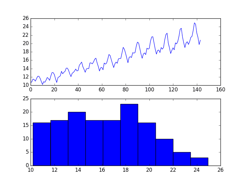
We can see that, as expected, the quadratic trend was made linear.
Square Root Transform of Quadratic Time Series
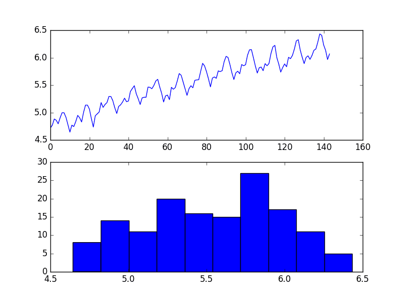
It is possible that the Airline Passengers dataset shows a quadratic growth. If this is the case, then we could expect a square root transform to reduce the growth trend to be linear and change the distribution of observations to be perhaps nearly Gaussian.
The example below performs a square root of the dataset and plots the results.
We can see that the trend was reduced, but was not removed.
The line plot still shows an increasing variance from cycle to cycle. The histogram still shows a long tail to the right of the distribution, suggesting an exponential or long-tail distribution.
Square Root Transform of Airline Passengers Dataset Plot
Log Transform
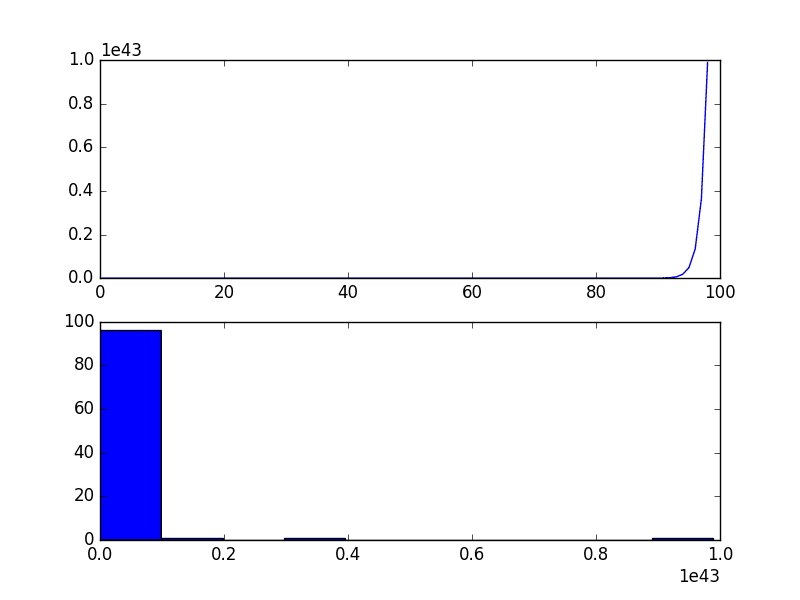
A class of more extreme trends are exponential, often graphed as a hockey stick.
Time series with an exponential distribution can be made linear by taking the logarithm of the values. This is called a log transform.
As with the square and square root case above, we can demonstrate this with a quick example.
The code below creates an exponential distribution by raising the numbers from 1 to 99 to the value e, which is the base of the natural logarithms or Euler’s number (2.718…).
1
2
3
4
5
6
7
8
9
10
11
from matplotlib import pyplot
from math import exp
series=[exp(i)foriinrange(1,100)]
pyplot.figure(1)
# line plot
pyplot.subplot(211)
pyplot.plot(series)
# histogram
pyplot.subplot(212)
pyplot.hist(series)
pyplot.show()
Running the example creates a line plot of the series and a histogram of the distribution of observations.
We see an extreme increase on the line graph and an equally extreme long tail distribution on the histogram.
Exponential Time Series
Again, we can transform this series back to linear by taking the natural logarithm of the values.
This would make the series linear and the distribution uniform. The example below demonstrates this for completeness.
1
2
3
4
5
6
7
8
9
10
11
12
13
from matplotlib import pyplot
from math import exp
from numpy import log
series=[exp(i)foriinrange(1,100)]
transform=log(series)
pyplot.figure(1)
# line plot
pyplot.subplot(211)
pyplot.plot(transform)
# histogram
pyplot.subplot(212)
pyplot.hist(transform)
pyplot.show()
Running the example creates plots, showing the expected linear result.
Log Transformed Exponential Time Series
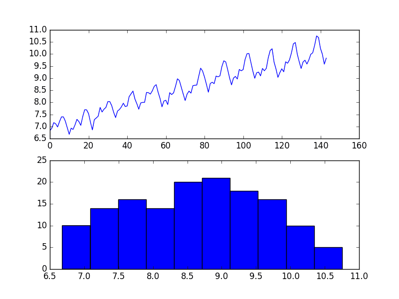
Our Airline Passengers dataset has a distribution of this form, but perhaps not this extreme.
The example below demonstrates a log transform of the Airline Passengers dataset.
Running the example results in a trend that does look a lot more linear than the square root transform above. The line plot shows a seemingly linear growth and variance.
The histogram also shows a more uniform or squashed Gaussian-like distribution of observations.
Log Transform of Airline Passengers Dataset Plot
Log transforms are popular with time series data as they are effective at removing exponential variance.
It is important to note that this operation assumes values are positive and non-zero. It is common to transform observations by adding a fixed constant to ensure all input values meet this requirement. For example:
1
transform = log(constant + x)
Where transform is the transformed series, constant is a fixed value that lifts all observations above zero, and x is the time series.
Box-Cox Transform
The square root transform and log transform belong to a class of transforms called power transforms.
The Box-Cox transform is a configurable data transform method that supports both square root and log transform, as well as a suite of related transforms.
More than that, it can be configured to evaluate a suite of transforms automatically and select a best fit. It can be thought of as a power tool to iron out power-based change in your time series. The resulting series may be more linear and the resulting distribution more Gaussian or Uniform, depending on the underlying process that generated it.
The scipy.stats library provides an implementation of the Box-Cox transform. The boxcox() function takes an argument, called lambda, that controls the type of transform to perform.
Below are some common values for lambda
lambda = -1. is a reciprocal transform.
lambda = -0.5 is a reciprocal square root transform.
lambda = 0.0 is a log transform.
lambda = 0.5 is a square root transform.
lambda = 1.0 is no transform.
For example, we can perform a log transform using the boxcox() function as follows:
Running the example discovers the lambda value of 0.148023.
We can see that this is very close to a lambda value of 0.0, resulting in a log transform and stronger (less than) than 0.5 for the square root transform.
1
Lambda: 0.148023
The line and histogram plots are also very similar to those from the log transform.
BoxCox Auto Transform of Airline Passengers Dataset Plot
Summary
In this tutorial, you discovered how to identify when to use and how to use different power transforms on time series data with Python.
Specifically, you learned:
How to identify a quadratic change and use the square root transform.
How to identify an exponential change and how to use the log transform.
How to use the Box-Cox transform to perform square root and log transforms and automatically optimize the transform for a dataset.
Do you have any questions about power transforms, or about this tutorial?
Ask your questions in the comments below and I will do my best to answer.
Want to Develop Time Series Forecasts with Python?
Thanks for this article. A lot of people write about log transformations and provide no explanation of when to not do a log transform, and Box-Cox fills in a lot of the gaps. Thanks!
A few follow up questions:
– Assuming the minimum value of a variable is > 0, are there situations in which you would not try and use Box-Cox? The scipy.stats.boxplot module will also decide when a transformation is unnecessary, so seems like there’s no harm in trying it for every variable. I’d imagine the main cost is loss of interpretability if you’re visualizing model results.
– In situations where you shouldn’t use a Box-Cox, what alternative transformations do you recommend?
Thanks for the blog. It’s very helpful for me since I’m currently working on a project where I need to log transform the data.
I have the following question, if I fit the transformed data to extract information such as the mean and variance or the forecasted value. Does scipy have a way to transform the data back?
Hi, thanks much for the tutorial.
When taking the square root of the airline, you say we expect the distribution to be Gaussian, while in the previous example with generated quadratic data, you expected a uniform distribution.
When will we expect one over the other ?
Thanks !
Hi Jason! Currently working on the e-book right now. Could you explain a bit how would a linear line plot will have a Gaussian distribution? Should it only create a uniform distribution? Thanks!
Much of the data I work with contains many zeros and is heavily skewed to the right. I have sometimes added a small value (like 0.1) to each record in order to perform a log transformation.
Can the Box-Cox package handle data that contains zeros?
Hi Jason, thanks for your blog.. It is good as like your other blog posts. However got a questions, if I use to box_cox to automatically use for transformation for my series, how can I convert it back..i meant transform back to original values..is there a function that does automatically as well?
nice one; i was interested in a first-principles explanation of Box-Cox; at university many years ago was the last time had this understanding. I don’t work in python so i didn’t use your code; however, your use of clear shot snippets to explain step-by-step what is B-C, is excellent
How do we inverse the log transformed data or time series back to the original time series scale?
Secondly, I used log transform on my time series data that shows exponential growth trends, to make it linear, and I had a histogram plot that is more uniform and Gaussian-like distribution. The log transform lifted model skills tremendously, but in log scale, rather than the original time series scale. In addition, I did not do any further transform on my time series data, even though, they contain zeroes and negative values. Does it really matter?
Thanks a lot for the great post. So my question is that, the box-cox algorithm helps to determine if there is any trend or seasonality. How do we remove that trend and make the time series stationary ? Do we need to substract the trend or seasonality factor from the original data set and feed to the ARIMA model to decide the value of p,q and d? If you have any article related to this, please share.
Also, for an ARIMA model, a stationary time series is mandatory ? I have a data set similar to the air passeneger data set. I have the data set from 2014 to 2017. I want to predict it for 2018.
Thank you for your post. It is very useful.
My time series data is multiplicative.
2 Questios::
1. What do I need to calculate log of? Dependent variable Y or Resduals r? To elaborate,
Once I calculate log(Y), should I then calculate residual as r = log(Y) /(trend x seasonality). Or should I calculate r = Y/(tend x seasonality) and then calculate log (r)?
2. If my trend and seasonality are independent variables (features) then should I also calculate log of them before doing
r = log(Y) /(trend x seasonality)
I want to transform Generalized Normal Distribution to Normal Distribution (through uniform distribution??, read from some literature, there not much ICDF is available for Gennorm). I follow similar technique of that you have indicated. Not able to get the required outcome!
Can you help me out please?
Let me see if I understand you correctly from a Mada’s question from above so I can avoid
any foobar-ing on my part. If I am doing ARIMA I should be doing the differencing BEFORE
applying Box_cox or Yeo? Then do Box_cox?
As always, it’s a treat reading your articles. Just a quick question.
I have seen people applying Box-Cox transform AFTER performing train-test split. Which is okay until there is not data leakage in pipeline. But is it really required to perform ANY transformation (including differences etc.) on test data? We anyways inverse transform the predictions generated using train data before actual model evaluation.
In short, you do we apply any transformation on test data when it’s supposed to be hidden during training?
Hello Jason, thanks for this awesome post! I’ve searched through the internet but am still confused about how we apply power transformation to multiple examples. Say if we have about 20 univariate datapoints of length 20, do we treat each datapoint as an independent feature or do we want to concatenate all of the datapoints since they are describing the same variable? Thanks!
If I have a time series with no general trend but a strong seasonality, and its distribution is bi-modal. What transform should I use ? Without any transforms, I have used a DNN and it pretty much works good but I am curious to know if there’s any room for improvement using transforms, if yes which one? Thanks!
Thank you for the prompt reply. Another doubt I had is about minmax scaler. In the case of scaling univariate time series to 0-1, we should treat each datapoint in training set as the same feature instead of each single datapoint as a feature, right? Otherwise we won’t have shared min/max parameter?
Hi Jason, I am reading your book on time-series. I wanted to ask you two questions:
1. Do we remove seasonality and trend before applying power transform?
2. Which power transform is better for data like the mean temperature of a city?
Dear Jason
I need to use Yeo–Johnson transformation for both negative and positive “one dimensional” data, as well as inverting the predicted values to their origins I couldn’t find an appropriate python code for it. please help me.
I am performing the box-cox method in my data and want to use it as a label for ML. It makes the error so low, yet I am skeptical about the procedure. Do I need to change the data back to the normal form for doing any further analysis? As the range of data becomes so compact( between 0.85 to 1) [although I am using percent error for my decision making] and in contrast with the low error, the predictions are in contrast with any common sense. I really appreciate your guidance.
Are there any issues for interpreting the results or confidence intervals while applying the inverse function? I ask because I notice the confidence interval will often no longer appear symmetrical after the exponentiated/inversed back to the original. How would one phrase the explanation to someone who is skeptical of the asymmetric confidence intervals?
Thank you for your article.
I applied the box cox transform and had : Lambda= 35.32, how can i interpret it ?
Also i would like to know how to reverse the box cox transform, once i will train my model i will need to rescale my data
Thank you.
If the data does not have trend or seasonality. Do I need to do the transformation. Its a huge data of about 1 lakh forty thousand rows. Hourly power consumption data from 2007 to 2018


Thanks for this article. A lot of people write about log transformations and provide no explanation of when to not do a log transform, and Box-Cox fills in a lot of the gaps. Thanks!
A few follow up questions:
– Assuming the minimum value of a variable is > 0, are there situations in which you would not try and use Box-Cox? The scipy.stats.boxplot module will also decide when a transformation is unnecessary, so seems like there’s no harm in trying it for every variable. I’d imagine the main cost is loss of interpretability if you’re visualizing model results.
– In situations where you shouldn’t use a Box-Cox, what alternative transformations do you recommend?
I agree, try, evaluate and adopt if a transform lifts skill. Often model skill is the goal for a project.
A “Yeo-Johnson transformation” can be used as an alternative to box-cox:
https://en.wikipedia.org/wiki/Power_transform#Yeo-Johnson_transformation
Thanks for the blog. It’s very helpful for me since I’m currently working on a project where I need to log transform the data.
I have the following question, if I fit the transformed data to extract information such as the mean and variance or the forecasted value. Does scipy have a way to transform the data back?
Off hand, I don’t think so.
You can invert the power transform if you know the lambda.
I show how here:
https://machinelearningmastery.com/machine-learning-data-transforms-for-time-series-forecasting/
Hi, thanks much for the tutorial.
When taking the square root of the airline, you say we expect the distribution to be Gaussian, while in the previous example with generated quadratic data, you expected a uniform distribution.
When will we expect one over the other ?
Thanks !
It really depends on the data.
Hi Jason! Currently working on the e-book right now. Could you explain a bit how would a linear line plot will have a Gaussian distribution? Should it only create a uniform distribution? Thanks!
Yes, this gives examples:
https://machinelearningmastery.com/a-gentle-introduction-to-normality-tests-in-python/
Please, help!
after writing the first code line from the first example I have got the following error message:
>>> from pandas import Series
Traceback (most recent call last):
File “”, line 1, in
from pandas import Series
ImportError: No module named pandas
>>>
You need to install Pandas. This tutorial will help you:
https://machinelearningmastery.com/setup-python-environment-machine-learning-deep-learning-anaconda/
Dear Jason, I love this tutorial!
Much of the data I work with contains many zeros and is heavily skewed to the right. I have sometimes added a small value (like 0.1) to each record in order to perform a log transformation.
Can the Box-Cox package handle data that contains zeros?
Thanks again for your great information 🙂
Generally, no.
Nevertheless, try it (with an offset to get all values >0) to see if it has an impact.
FYI – scipy.stats.boxcox is buggy. 🙁
Why do you say that?
This thread shows the problem. I ran into the problem running your code but on my data.
https://github.com/scipy/scipy/issues/6873
The problem occurs when stats.boxcox calls stats.boxcox_normmax Very annoying.
Sorry to hear that.
Hi Jason, thanks for your blog.. It is good as like your other blog posts. However got a questions, if I use to box_cox to automatically use for transformation for my series, how can I convert it back..i meant transform back to original values..is there a function that does automatically as well?
You can invert the process with a function like the following:
nice one; i was interested in a first-principles explanation of Box-Cox; at university many years ago was the last time had this understanding. I don’t work in python so i didn’t use your code; however, your use of clear shot snippets to explain step-by-step what is B-C, is excellent
Thanks Doug, I’m happy it was useful.
Hi Jason,
How do we inverse the log transformed data or time series back to the original time series scale?
Secondly, I used log transform on my time series data that shows exponential growth trends, to make it linear, and I had a histogram plot that is more uniform and Gaussian-like distribution. The log transform lifted model skills tremendously, but in log scale, rather than the original time series scale. In addition, I did not do any further transform on my time series data, even though, they contain zeroes and negative values. Does it really matter?
Regards,
Kingsley
Thanks
The inverse of log is exp()
The transforms required really depend on your data.
Thanks
I’m happy that it helped.
Hi Jason,
Thanks a lot for the great post. So my question is that, the box-cox algorithm helps to determine if there is any trend or seasonality. How do we remove that trend and make the time series stationary ? Do we need to substract the trend or seasonality factor from the original data set and feed to the ARIMA model to decide the value of p,q and d? If you have any article related to this, please share.
Also, for an ARIMA model, a stationary time series is mandatory ? I have a data set similar to the air passeneger data set. I have the data set from 2014 to 2017. I want to predict it for 2018.
Your help will be highly appreciated 🙂
No, box-cox shifts a data distribution to be more Gaussian.
You can remove a trend using a difference transform.
When using ARIMA, it can perform this differencing for you.
Thank you for your post. It is very useful.
My time series data is multiplicative.
2 Questios::
1. What do I need to calculate log of? Dependent variable Y or Resduals r? To elaborate,
Once I calculate log(Y), should I then calculate residual as r = log(Y) /(trend x seasonality). Or should I calculate r = Y/(tend x seasonality) and then calculate log (r)?
2. If my trend and seasonality are independent variables (features) then should I also calculate log of them before doing
r = log(Y) /(trend x seasonality)
You transform the raw data that you’re modeling.
I recommend subtracting the trend and seasonality from the data first, e.g. make the series stationary.
But if I substract seasonality and trend then it will make the data negative? And you mentioned calculating log of negative data isn’t allowed
You can force the data to be positive by adding an offset.
Hi Jason,
Currently working through your eBook on TimeSeries. Learned loads already, very exciting.
If I run the code of the Box-Cox with optimized Lambda, my Lambda is optimized for 8.4.
Have you seen this issue before?
Thanks,
Thomas
Wow, that is a massive value.
No, I have not seen that before.
Hi Dr Jason,
Good article!!
I want to transform Generalized Normal Distribution to Normal Distribution (through uniform distribution??, read from some literature, there not much ICDF is available for Gennorm). I follow similar technique of that you have indicated. Not able to get the required outcome!
Can you help me out please?
Sorry, I don’t have a tutorial on this topic – I don’t have good off the cuff advice.
Hi. Useful post. Thank-you.
Let me see if I understand you correctly from a Mada’s question from above so I can avoid
any foobar-ing on my part. If I am doing ARIMA I should be doing the differencing BEFORE
applying Box_cox or Yeo? Then do Box_cox?
Thanks.
Yes, differencing first. I outline a suggested ordering here:
https://machinelearningmastery.com/machine-learning-data-transforms-for-time-series-forecasting/
Hi Jason,
As always, it’s a treat reading your articles. Just a quick question.
I have seen people applying Box-Cox transform AFTER performing train-test split. Which is okay until there is not data leakage in pipeline. But is it really required to perform ANY transformation (including differences etc.) on test data? We anyways inverse transform the predictions generated using train data before actual model evaluation.
In short, you do we apply any transformation on test data when it’s supposed to be hidden during training?
Thanks.
Correct. Calculate on training, apply to train, test, and any other data.
Hello Jason,
Great tutorial! Will the transforms hold good if I’m performing time series classification?
Perhaps develop a prototype for your dataset and discover the answer.
Thank you very much! I will try it out!!
You’re welcome.
Hello Jason, thanks for this awesome post! I’ve searched through the internet but am still confused about how we apply power transformation to multiple examples. Say if we have about 20 univariate datapoints of length 20, do we treat each datapoint as an independent feature or do we want to concatenate all of the datapoints since they are describing the same variable? Thanks!
Each “series” would be a separate input feature:
https://machinelearningmastery.com/faq/single-faq/what-is-the-difference-between-samples-timesteps-and-features-for-lstm-input
Hi Jason,
If I have a time series with no general trend but a strong seasonality, and its distribution is bi-modal. What transform should I use ? Without any transforms, I have used a DNN and it pretty much works good but I am curious to know if there’s any room for improvement using transforms, if yes which one? Thanks!
Seasonal transform to remove the seasonality.
Thank you for the prompt reply. Another doubt I had is about minmax scaler. In the case of scaling univariate time series to 0-1, we should treat each datapoint in training set as the same feature instead of each single datapoint as a feature, right? Otherwise we won’t have shared min/max parameter?
Correct.
Hi Jason, I am reading your book on time-series. I wanted to ask you two questions:
1. Do we remove seasonality and trend before applying power transform?
2. Which power transform is better for data like the mean temperature of a city?
Thanks in advance!
Great questions.
Yes. This can help with the order of transforms:
https://machinelearningmastery.com/machine-learning-data-transforms-for-time-series-forecasting/
Perhaps test a few transforms and discover which results in a better performing model on your dataset.
My time series experienced a huge fall in values that makes it non-stationary.
I got a lambda value =1 which means no transformation is needed. However, the time series is still non-stationary.
What should I do for time series with abrupt change?
I believe they call this a regime change. Perhaps there are techniques designed specifically for that, you can try checking the literature.
Perhaps manually separate the data before and after the change in level and model them as separate problems.
Hi, your code for log transform in airplane is wrong, because it has some errors
Sorry to hear that you are having problems running the code, perhaps this will help:
https://machinelearningmastery.com/faq/single-faq/why-does-the-code-in-the-tutorial-not-work-for-me
Dear Jason
I need to use Yeo–Johnson transformation for both negative and positive “one dimensional” data, as well as inverting the predicted values to their origins I couldn’t find an appropriate python code for it. please help me.
See this example:
https://machinelearningmastery.com/power-transforms-with-scikit-learn/
I am performing the box-cox method in my data and want to use it as a label for ML. It makes the error so low, yet I am skeptical about the procedure. Do I need to change the data back to the normal form for doing any further analysis? As the range of data becomes so compact( between 0.85 to 1) [although I am using percent error for my decision making] and in contrast with the low error, the predictions are in contrast with any common sense. I really appreciate your guidance.
Thanks
Yes, the transform must be inverted on expected and predicted values before calculating an error value in the original units.
Are there any issues for interpreting the results or confidence intervals while applying the inverse function? I ask because I notice the confidence interval will often no longer appear symmetrical after the exponentiated/inversed back to the original. How would one phrase the explanation to someone who is skeptical of the asymmetric confidence intervals?
Hi Thom…Please rephrase your question. Not sure what you are attempting to differently from the examples provided.
Hi Jason big fan!!
was facing an issue, how to invert a yeo johnson transfomation to get original values back
Hi Jason big fan!!
was facing an issue, how to do inverse transform of yeo johnson transfomation to get original values back
Thank you for the support Asimov!
Hi,
Thank you for your article.
I applied the box cox transform and had : Lambda= 35.32, how can i interpret it ?
Also i would like to know how to reverse the box cox transform, once i will train my model i will need to rescale my data
Thank you.
Hi Nadine…you may find the following helpful:
https://www.codegrepper.com/code-examples/python/inverse+box-cox+transformation+python
https://towardsdatascience.com/box-cox-transformation-explained-51d745e34203
Hi,
If the data does not have trend or seasonality. Do I need to do the transformation. Its a huge data of about 1 lakh forty thousand rows. Hourly power consumption data from 2007 to 2018
Hi Ankitha…You may wish to consider not transforming the data and using an LSTM model for your purpose. The following is a great starting point:
https://machinelearningmastery.com/use-timesteps-lstm-networks-time-series-forecasting/
Great article. Do these transforms serve the same purpose as differencing?
Hi US…You are very welcome! Yes. More can be found here:
https://machinelearningmastery.com/difference-time-series-dataset-python/
I read this article as well. Can you elaborate how you would decide whether to go for a power transform vs differencing?