The progressive growing generative adversarial network is an approach for training a deep convolutional neural network model for generating synthetic images.
It is an extension of the more traditional GAN architecture that involves incrementally growing the size of the generated image during training, starting with a very small image, such as a 4×4 pixels. This allows the stable training and growth of GAN models capable of generating very large high-quality images, such as images of synthetic celebrity faces with the size of 1024×1024 pixels.
In this tutorial, you will discover how to develop progressive growing generative adversarial network models from scratch with Keras.
After completing this tutorial, you will know:
How to develop pre-defined discriminator and generator models at each level of output image growth.
How to define composite models for training the generator models via the discriminator models.
How to cycle the training of fade-in version and normal versions of models at each level of output image growth.
How to Implement Progressive Growing GAN Models in Keras Photo by Diogo Santos Silva, some rights reserved.
Tutorial Overview
This tutorial is divided into five parts; they are:
What Is the Progressive Growing GAN Architecture?
How to Implement the Progressive Growing GAN Discriminator Model
How to Implement the Progressive Growing GAN Generator Model
How to Implement Composite Models for Updating the Generator
How to Train Discriminator and Generator Models
What Is the Progressive Growing GAN Architecture?
GANs are effective at generating crisp synthetic images, although are typically limited in the size of the images that can be generated.
The Progressive Growing GAN is an extension to the GAN that allows the training of generator models capable of outputting large high-quality images, such as photorealistic faces with the size 1024×1024 pixels. It was described in the 2017 paper by Tero Karras, et al. from Nvidia titled “Progressive Growing of GANs for Improved Quality, Stability, and Variation.”
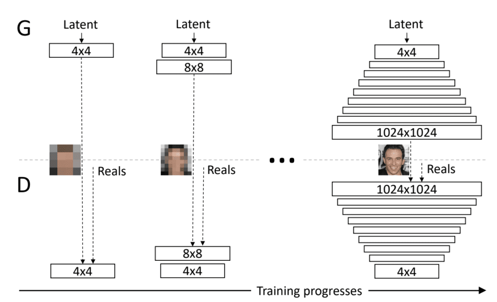
The key innovation of the Progressive Growing GAN is the incremental increase in the size of images output by the generator starting with a 4×4 pixel image and double to 8×8, 16×16, and so on until the desired output resolution.
Our primary contribution is a training methodology for GANs where we start with low-resolution images, and then progressively increase the resolution by adding layers to the networks.
This is achieved by a training procedure that involves periods of fine-tuning the model with a given output resolution, and periods of slowly phasing in a new model with a larger resolution.
When doubling the resolution of the generator (G) and discriminator (D) we fade in the new layers smoothly
Progressive Growing GAN involves using a generator and discriminator model with the same general structure and starting with very small images. During training, new blocks of convolutional layers are systematically added to both the generator model and the discriminator models.
Example of Progressively Adding Layers to Generator and Discriminator Models. Taken from: Progressive Growing of GANs for Improved Quality, Stability, and Variation.
The incremental addition of the layers allows the models to effectively learn coarse-level detail and later learn ever finer detail, both on the generator and discriminator side.
This incremental nature allows the training to first discover the large-scale structure of the image distribution and then shift attention to increasingly finer-scale detail, instead of having to learn all scales simultaneously.
The model architecture is complex and cannot be implemented directly.
In this tutorial, we will focus on how the progressive growing GAN can be implemented using the Keras deep learning library.
We will step through how each of the discriminator and generator models can be defined, how the generator can be trained via the discriminator model, and how each model can be updated during the training process.
These implementation details will provide the basis for you developing a progressive growing GAN for your own applications.
Want to Develop GANs from Scratch?
Take my free 7-day email crash course now (with sample code).
Click to sign-up and also get a free PDF Ebook version of the course.
How to Implement the Progressive Growing GAN Discriminator Model
The discriminator model is given images as input and must classify them as either real (from the dataset) or fake (generated).
During the training process, the discriminator must grow to support images with ever-increasing size, starting with 4×4 pixel color images and doubling to 8×8, 16×16, 32×32, and so on.
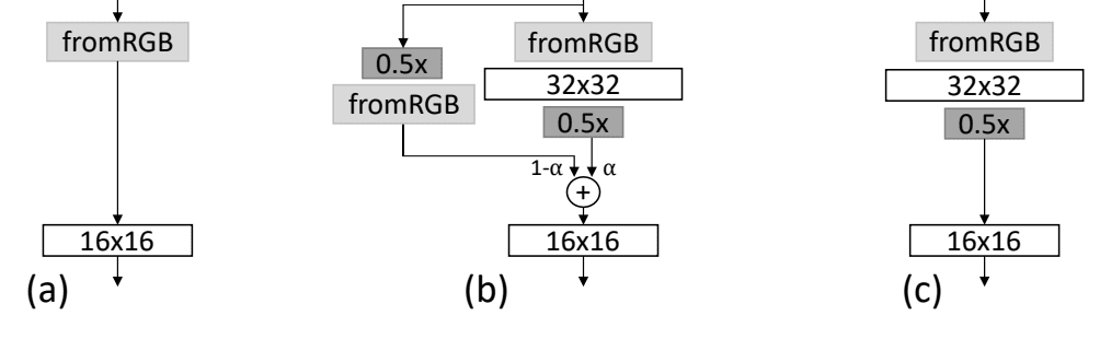
This is achieved by inserting a new input layer to support the larger input image followed by a new block of layers. The output of this new block is then downsampled. Additionally, the new image is also downsampled directly and passed through the old input processing layer before it is combined with the output of the new block.
During the transition from a lower resolution to a higher resolution, e.g. 16×16 to 32×32, the discriminator model will have two input pathways as follows:
The output of the new block that is downsampled and the output of the old input processing layer are combined using a weighted average, where the weighting is controlled by a new hyperparameter called alpha. The weighted sum is calculated as follows:
The weighted average of the two pathways is then fed into the rest of the existing model.
Initially, the weighting is completely biased towards the old input processing layer (alpha=0) and is linearly increased over training iterations so that the new block is given more weight until eventually, the output is entirely the product of the new block (alpha=1). At this time, the old pathway can be removed.
This can be summarized with the following figure taken from the paper showing a model before growing (a), during the phase-in of the larger resolution (b), and the model after the phase-in (c).
Figure Showing the Growing of the Discriminator Model, Before (a) During (b) and After (c) the Phase-In of a High Resolution. Taken from: Progressive Growing of GANs for Improved Quality, Stability, and Variation.
The fromRGB layers are implemented as a 1×1 convolutional layer. A block is comprised of two convolutional layers with 3×3 sized filters and the leaky ReLU activation function with a slope of 0.2, followed by a downsampling layer. Average pooling is used for downsampling, which is unlike most other GAN models that use transpose convolutional layers.
The output of the model involves two convolutional layers with 3×3 and 4×4 sized filters and Leaky ReLU activation, followed by a fully connected layer that outputs the single value prediction. The model uses a linear activation function instead of a sigmoid activation function like other discriminator models and is trained directly either by Wasserstein loss (specifically WGAN-GP) or least squares loss; we will use the latter in this tutorial. Model weights are initialized using He Gaussian (he_normal), which is very similar to the method used in the paper.
The model uses a custom layer called Minibatch standard deviation at the beginning of the output block, and instead of batch normalization, each layer uses local response normalization, referred to as pixel-wise normalization in the paper. We will leave out the minibatch normalization and use batch normalization in this tutorial for brevity.
One approach to implementing the progressive growing GAN would be to manually expand a model on demand during training. Another approach is to pre-define all of the models prior to training and carefully use the Keras functional API to ensure that layers are shared across the models and continue training.
I believe the latter approach might be easier and is the approach we will use in this tutorial.
First, we must define a custom layer that we can use when fading in a new higher-resolution input image and block. This new layer must take two sets of activation maps with the same dimensions (width, height, channels) and add them together using a weighted sum.
We can implement this as a new layer called WeightedSum that extends the Add merge layer and uses a hyperparameter ‘alpha‘ to control the contribution of each input. This new class is defined below. The layer assumes only two inputs: the first for the output of the old or existing layers and the second for the newly added layers. The new hyperparameter is defined as a backend variable, meaning that we can change it any time via changing the value of the variable.
The discriminator model is by far more complex than the generator to grow because we have to change the model input, so let’s step through this slowly.
Firstly, we can define a discriminator model that takes a 4×4 color image as input and outputs a prediction of whether the image is real or fake. The model is comprised of a 1×1 input processing layer (fromRGB) and an output block.
Next, we need to define a new model that handles the intermediate stage between this model and a new discriminator model that takes 8×8 color images as input.
The existing input processing layer must receive a downsampled version of the new 8×8 image. A new input process layer must be defined that takes the 8×8 input image and passes it through a new block of two convolutional layers and a downsampling layer. The output of the new block after downsampling and the old input processing layer must be added together using a weighted sum via our new WeightedSum layer and then must reuse the same output block (two convolutional layers and the output layer).
Given the first defined model and our knowledge about this model (e.g. the number of layers in the input processing layer is 2 for the Conv2D and LeakyReLU), we can construct this new intermediate or fade-in model using layer indexes from the old model.
We also need a version of the same model with the same layers without the fade-in of the input from the old model’s input processing layers.
This straight-through version is required for training before we fade-in the next doubling of the input image size.
We can update the above example to create two versions of the model. First, the straight-through version as it is simpler, then the version used for the fade-in that reuses the layers from the new block and the output layers of the old model.
The add_discriminator_block() function below implements this, returning a list of the two defined models (straight-through and fade-in), and takes the old model as an argument and defines the number of input layers as a default argument (3).
To ensure that the WeightedSum layer works correctly, we have fixed all convolutional layers to always have 64 filters, and in turn, output 64 feature maps. If there is a mismatch between the old model’s input processing layer and the new blocks output in terms of the number of feature maps (channels), then the weighted sum will fail.
It is not an elegant function as we have some repetition, but it is readable and will get the job done.
We can then call this function again and again as we double the size of input images. Importantly, the function expects the straight-through version of the prior model as input.
The example below defines a new function called define_discriminator() that defines our base model that expects a 4×4 color image as input, then repeatedly adds blocks to create new versions of the discriminator model each time that expects images with quadruple the area.
1
2
3
4
5
6
7
8
9
10
11
12
13
14
15
16
17
18
19
20
21
22
23
24
25
26
27
28
29
30
31
32
33
34
# define the discriminator models for each image resolution
This function will return a list of models, where each item in the list is a two-element list that contains first the straight-through version of the model at that resolution, and second the fade-in version of the model for that resolution.
We can tie all of this together and define a new “discriminator model” that will grow from 4×4, through to 8×8, and finally to 16×16. This is achieved by passing he n_blocks argument to 3 when calling the define_discriminator() function, for the creation of three sets of models.
The complete example is listed below.
1
2
3
4
5
6
7
8
9
10
11
12
13
14
15
16
17
18
19
20
21
22
23
24
25
26
27
28
29
30
31
32
33
34
35
36
37
38
39
40
41
42
43
44
45
46
47
48
49
50
51
52
53
54
55
56
57
58
59
60
61
62
63
64
65
66
67
68
69
70
71
72
73
74
75
76
77
78
79
80
81
82
83
84
85
86
87
88
89
90
91
92
93
94
95
96
97
98
99
100
101
102
103
104
105
106
107
108
109
110
111
112
# example of defining discriminator models for the progressive growing gan
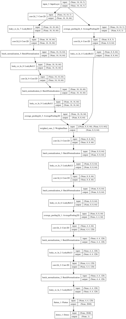
A plot of the same fade-in version of the model is created and saved to file.
Note: creating this plot assumes that the pygraphviz and pydot libraries are installed. If this is a problem, comment out the import statement and call to plot_model().
The plot shows the 16×16 input image that is downsampled and passed through the 8×8 input processing layers from the prior model (left). It also shows the addition of the new block (right) and the weighted average that combines both streams of input, before using the existing model layers to continue processing and outputting a prediction.
Plot of the Fade-In Discriminator Model For the Progressive Growing GAN Transitioning From 8×8 to 16×16 Input Images
Now that we have seen how we can define the discriminator models, let’s look at how we can define the generator models.
How to Implement the Progressive Growing GAN Generator Model
The generator models for the progressive growing GAN are easier to implement in Keras than the discriminator models.
The reason for this is because each fade-in requires a minor change to the output of the model.
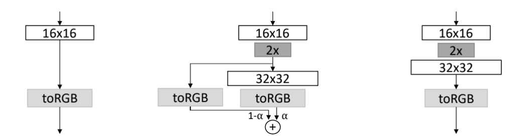
Increasing the resolution of the generator involves first upsampling the output of the end of the last block. This is then connected to the new block and a new output layer for an image that is double the height and width dimensions or quadruple the area. During the phase-in, the upsampling is also connected to the output layer from the old model and the output from both output layers is merged using a weighted average.
After the phase-in is complete, the old output layer is removed.
This can be summarized with the following figure, taken from the paper showing a model before growing (a), during the phase-in of the larger resolution (b), and the model after the phase-in (c).
Figure Showing the Growing of the Generator Model, Before (a), During (b), and After (c) the Phase-In of a High Resolution. Taken from: Progressive Growing of GANs for Improved Quality, Stability, and Variation.
The toRGB layer is a convolutional layer with 3 1×1 filters, sufficient to output a color image.
The model takes a point in the latent space as input, e.g. such as a 100-element or 512-element vector as described in the paper. This is scaled up to provided the basis for 4×4 activation maps, followed by a convolutional layer with 4×4 filters and another with 3×3 filters. Like the discriminator, LeakyReLU activations are used, as is pixel normalization, which we will substitute with batch normalization for brevity.
A block involves an upsample layer followed by two convolutional layers with 3×3 filters. Upsampling is achieved using a nearest neighbor method (e.g. duplicating input rows and columns) via a UpSampling2D layer instead of the more common transpose convolutional layer.
We can define the baseline model that will take a point in latent space as input and output a 4×4 color image as follows:
Next, we need to define a version of the model that uses all of the same input layers, although adds a new block (upsample and 2 convolutional layers) and a new output layer (a 1×1 convolutional layer).
This would be the model after the phase-in to the new output resolution. This can be achieved by using own knowledge about the baseline model and that the end of the last block is the second last layer, e.g. layer at index -2 in the model’s list of layers.
The new model with the addition of a new block and output layer is defined as follows:
That is pretty straightforward; we have chopped off the old output layer at the end of the last block and grafted on a new block and output layer.
Now we need a version of this new model to use during the fade-in.
This involves connecting the old output layer to the new upsampling layer at the start of the new block and using an instance of our WeightedSum layer defined in the previous section to combine the output of the old and new output layers.
1
2
3
4
5
6
7
8
9
...
# get the output layer from old model
out_old=old_model.layers[-1]
# connect the upsampling to the old output layer
out_image2=out_old(upsampling)
# define new output image as the weighted sum of the old and new models
merged=WeightedSum()([out_image2,out_image])
# define model
model2=Model(old_model.input,merged)
We can combine the definition of these two operations into a function named add_generator_block(), defined below, that will expand a given model and return both the new generator model with the added block (model1) and a version of the model with the fading in of the new block with the old output layer (model2).
# define new output image as the weighted sum of the old and new models
merged=WeightedSum()([out_image2,out_image])
# define model
model2=Model(old_model.input,merged)
return[model1,model2]
We can then call this function with our baseline model to create models with one added block and continue to call it with subsequent models to keep adding blocks.
The define_generator() function below implements this, taking the size of the latent space and number of blocks to add (models to create).
The baseline model is defined as outputting a color image with the shape 4×4, controlled by the default argument in_dim.
We can tie all of this together and define a baseline generator and the addition of two blocks, so three models in total, where a straight-through and fade-in version of each model is defined.
The complete example is listed below.
1
2
3
4
5
6
7
8
9
10
11
12
13
14
15
16
17
18
19
20
21
22
23
24
25
26
27
28
29
30
31
32
33
34
35
36
37
38
39
40
41
42
43
44
45
46
47
48
49
50
51
52
53
54
55
56
57
58
59
60
61
62
63
64
65
66
67
68
69
70
71
72
73
74
75
76
77
78
79
80
81
82
83
84
85
86
87
88
89
90
91
92
# example of defining generator models for the progressive growing gan
The example chooses the fade-in model for the last model to summarize.
Running the example first summarizes a linear list of the layers in the model. We can see that the last model takes a point from the latent space and outputs a 16×16 image.
This matches as our expectations as the baseline model outputs a 4×4 image, adding one block increases this to 8×8, and adding one more block increases this to 16×16.
A plot of the same fade-in version of the model is created and saved to file.
Note: creating this plot assumes that the pygraphviz and pydot libraries are installed. If this is a problem, comment out the import statement and call to plot_model().
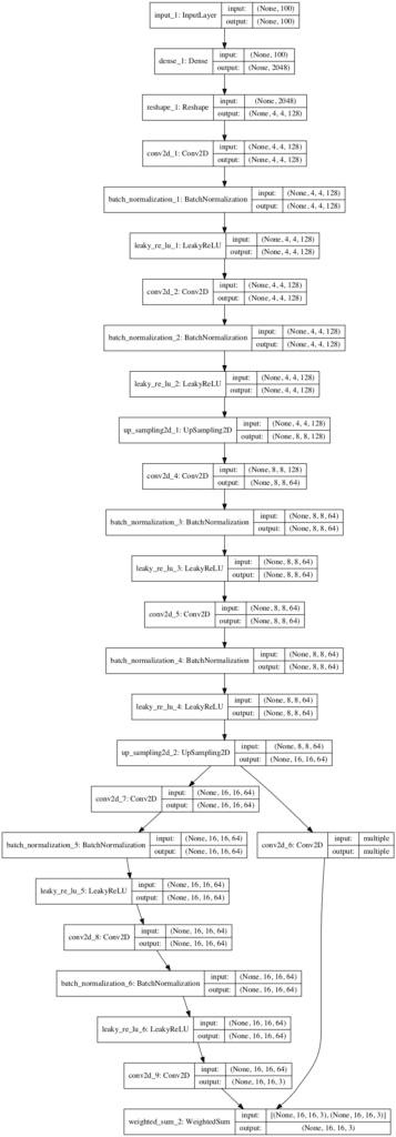
We can see that the output from the last block passes through an UpSampling2D layer before feeding the added block and a new output layer as well as the old output layer before being merged via a weighted sum into the final output layer.
Plot of the Fade-In Generator Model For the Progressive Growing GAN Transitioning From 8×8 to 16×16 Output Images
Now that we have seen how to define the generator models, we can review how the generator models may be updated via the discriminator models.
How to Implement Composite Models for Updating the Generator
The discriminator models are trained directly with real and fake images as input and a target value of 0 for fake and 1 for real.
The generator models are not trained directly; instead, they are trained indirectly via the discriminator models, just like a normal GAN model.
We can create a composite model for each level of growth of the model, e.g. pair 4×4 generators and 4×4 discriminators. We can also pair the straight-through models together, and the fade-in models together.
For example, we can retrieve the generator and discriminator models for a given level of growth.
1
2
...
g_models,d_models=generators[0],discriminators[0]
Then we can use them to create a composite model for training the straight-through generator, where the output of the generator is fed directly to the discriminator in order to classify.
The function below, named define_composite(), automates this; given a list of defined discriminator and generator models, it will create an appropriate composite model for training each generator model.
1
2
3
4
5
6
7
8
9
10
11
12
13
14
15
16
17
18
19
20
21
# define composite models for training generators via discriminators
Tying this together with the definition of the discriminator and generator models above, the complete example of defining all models at each pre-defined level of growth is listed below.
1
2
3
4
5
6
7
8
9
10
11
12
13
14
15
16
17
18
19
20
21
22
23
24
25
26
27
28
29
30
31
32
33
34
35
36
37
38
39
40
41
42
43
44
45
46
47
48
49
50
51
52
53
54
55
56
57
58
59
60
61
62
63
64
65
66
67
68
69
70
71
72
73
74
75
76
77
78
79
80
81
82
83
84
85
86
87
88
89
90
91
92
93
94
95
96
97
98
99
100
101
102
103
104
105
106
107
108
109
110
111
112
113
114
115
116
117
118
119
120
121
122
123
124
125
126
127
128
129
130
131
132
133
134
135
136
137
138
139
140
141
142
143
144
145
146
147
148
149
150
151
152
153
154
155
156
157
158
159
160
161
162
163
164
165
166
167
168
169
170
171
172
173
174
175
176
177
178
179
180
181
182
183
184
185
186
187
188
189
190
191
192
193
194
195
# example of defining composite models for the progressive growing gan
Now that we know how to define all of the models, we can review how the models might be updated during training.
How to Train Discriminator and Generator Models
Pre-defining the generator, discriminator, and composite models was the hard part; training the models is straight forward and much like training any other GAN.
Importantly, in each training iteration the alpha variable in each WeightedSum layer must be set to a new value. This must be set for the layer in both the generator and discriminator models and allows for the smooth linear transition from the old model layers to the new model layers, e.g. alpha values set from 0 to 1 over a fixed number of training iterations.
The update_fadein() function below implements this and will loop through a list of models and set the alpha value on each based on the current step in a given number of training steps. You may be able to implement this more elegantly using a callback.
1
2
3
4
5
6
7
8
9
# update the alpha value on each instance of WeightedSum
def update_fadein(models,step,n_steps):
# calculate current alpha (linear from 0 to 1)
alpha=step/float(n_steps-1)
# update the alpha for each model
formodel inmodels:
forlayer inmodel.layers:
ifisinstance(layer,WeightedSum):
backend.set_value(layer.alpha,alpha)
We can define a generic function for training a given generator, discriminator, and composite model for a given number of training epochs.
The train_epochs() function below implements this where first the discriminator model is updated on real and fake images, then the generator model is updated, and the process is repeated for the required number of training iterations based on the dataset size and the number of epochs.
This function calls helper functions for retrieving a batch of real images via generate_real_samples(), generating a batch of fake samples with the generator generate_fake_samples(), and generating a sample of points in latent space generate_latent_points(). You can define these functions yourself quite trivially.
The images must be scaled to the size of each model. If the images are in-memory, we can define a simple scale_dataset() function to scale the loaded images.
In this case, we are using the skimage.transform.resize function from the scikit-image library to resize the NumPy array of pixels to the required size and use nearest neighbor interpolation.
1
2
3
4
5
6
7
8
9
# scale images to preferred size
def scale_dataset(images,new_shape):
images_list=list()
forimage inimages:
# resize with nearest neighbor interpolation
new_image=resize(image,new_shape,0)
# store
images_list.append(new_image)
returnasarray(images_list)
First, the baseline model must be fit for a given number of training epochs, e.g. the model that outputs 4×4 sized images.
This will require that the loaded images be scaled to the required size defined by the shape of the generator models output layer.
We can then process each level of growth, e.g. the first being 8×8.
This involves first retrieving the models, scaling the data to the appropriate size, then fitting the fade-in model followed by training the straight-through version of the model for fine tuning.
We can repeat this for each level of growth in a loop.
The number of epochs for the normal phase is defined by the e_norm argument and the number of epochs during the fade-in phase is defined by the e_fadein argument.
The number of epochs must be specified based on the size of the image dataset and the same number of epochs can be used for each phase, as was used in the paper.
We start with 4×4 resolution and train the networks until we have shown the discriminator 800k real images in total. We then alternate between two phases: fade in the first 3-layer block during the next 800k images, stabilize the networks for 800k images, fade in the next 3-layer block during 800k images, etc.
thanks for your implementation of the progressive GANs paper. I was looking through the code and have this question. For each new resolution, you use the generators and discriminators from g_models[i] and d_models[i]. Are the weights from the previous resolution loaded prior to training at a higher resolution? I checked the function train_epoch and the code block prior to it, but the previously trained weights don’t seem to be explicitly loaded before training a new resolution.
Just to clarify, for example, you train g_normal (g_model[0][0]). The next round trains g_model[1][0]. Isn’t that another instance with untrained weights? How are the previously trained weights reused? Thanks for helping!
No, we are grafting on new layers to existing layers and defining a new model with those layers. The weights don’t change – all the layers point to the same matrix in memory across the models.
Thanks very much for explaining it! The weights at the higher resolutions do indeed use the weights learned during training at lower resolutions. Great work!
I think that inserting the upsampling before old output layer in generator is wrong, because you training this layer with old shape (straight model), and then you training this layer in fadein model with another shape (thats why you get “multiple” value for this layer in “output shape” column of plotted graph). You need to insert upsampling after old conv in the right branch and before new conv in the left branch.
to_rgb is 1×1 conv, so it is just a weighted sum of layer’s feature maps per channel, so it does not matter whether it is before or after upsampling (in this case). Placing upsampling before old output layer is more optimal, because we can do it once instead of doing it twice, and get the same result.
I have a problem with the output of the generator.
Without defining an activation layer, I obtain images with negative values.
If I add an activation layer (sigmoid) I encounter problems during fedein phase.
What is the best practice to avoid this problem?
Hi, You always create great tutorials I always read your topiks. I have a question i am new in GAN area and I am just began to study, and i have some confused. I have trained DCGAN model and save the model, after training i want to used this model and create new image. How can i create new image using exist model. I do not know how to call the exist model and generate new image. Thank you
Hi Jason,
I am implementing Progressive Growing GAN to generate fake photo-realistic computer graphic images. when i run the following code, i am getting an error name ‘alpha’ is not defined. please help me in this regard.
# weighted sum output
class WeightedSum(Add):
# init with default value
def __init__(self, alpha=0.0, **kwargs):
super(WeightedSum, self).__init__(**kwargs)
self.alpha = backend.variable(alpha, name=’ws_alpha’)
# output a weighted sum of inputs
def _merge_function(self, inputs):
# only supports a weighted sum of two inputs
assert (len(inputs) == 2)
# ((1-a) * input1) + (a * input2)
output = ((1.0 – self.alpha) * inputs[0]) + (self.alpha * inputs[1])
return output
after few hours of investigation i found that the learning rate caused the problem with the bad outputs and loss that reached 3000, the learning rate should be something like 0.0002 and in this tutorial its 0.001.
Do you know under which condition the training converges? Do you have a condition in your code that stops the training? If so, can you point to me? Also, do we have to handle the case when the alpha in weighted sum reaches 1? we have to stop updating alpha, otherwise it will grow higher than 1.
Hi, I tried running the full example of discriminator. It looks like for the first layer (4×4) the model appends 2 models of straight through discriminator rather than one straight through and one a fade in version. Is this correct or have I misunderstood something?
One common mistake that I have noticed in this (and many other) implementation of Prog GAN is that it does not consist the equalized learning rate (or at least I don’t see it). The reason why it is so important is that it makes Prog GAN very stable, and results are much better. Instead of initializing weights using He initialization, authors initialize them with random normal distribution and whenever weights are called, they are multiplied by a constant from He initialization, but this constant is not updated via gradient descent, only weights are being updated. Without this, the learning rate can get both too small and too large due to progressive growth.
Snaily said this was related to the version of TensorFlow. I am running this in google colab with TF version 2.7.0. Could this be the issue? What version was this written in?


 From Scratch with Keras")
 From Scratch in Keras")
Hello,
I’m new at M/L.
I’ve a question about predict in Keras.
I’ve the following snippet of code.
predictions = model.predict(test_images)
predictions[0]
np.argmax(predictions[0])
WHY I have to use predictions[0] (and WHY “0”) instead of using only predictions.
I dont’ really understand.
Thanks a lot
Perhaps this will help:
https://machinelearningmastery.com/how-to-make-classification-and-regression-predictions-for-deep-learning-models-in-keras/
Thanks for your help.
I’ve one more question. Is there any tutorial about using LSTM with Keras?
Thanks a lot
Yes, I have hundreds. Get started here:
https://machinelearningmastery.com/start-here/#lstm
For time series and LSTM here:
https://machinelearningmastery.com/start-here/#deep_learning_time_series
Hi
Could you please explain what downsampling exactly means?
Thanks!
To use statistical methods to go from a larger resolution to a smaller resolution.
Great article, do you happen to have a link to the notebook?
I don’t use notebooks and recommend not using them, here’s why:
https://machinelearningmastery.com/faq/single-faq/why-dont-use-or-recommend-notebooks
Hi Jason,
thanks for your implementation of the progressive GANs paper. I was looking through the code and have this question. For each new resolution, you use the generators and discriminators from g_models[i] and d_models[i]. Are the weights from the previous resolution loaded prior to training at a higher resolution? I checked the function train_epoch and the code block prior to it, but the previously trained weights don’t seem to be explicitly loaded before training a new resolution.
Cheers!
The weights are reused in the new model.
That is, we build the new model using the parts of the old model – including their weights.
Does that help?
Just to clarify, for example, you train g_normal (g_model[0][0]). The next round trains g_model[1][0]. Isn’t that another instance with untrained weights? How are the previously trained weights reused? Thanks for helping!
No, we are grafting on new layers to existing layers and defining a new model with those layers. The weights don’t change – all the layers point to the same matrix in memory across the models.
Thanks very much for explaining it! The weights at the higher resolutions do indeed use the weights learned during training at lower resolutions. Great work!
Thanks.
I think that inserting the upsampling before old output layer in generator is wrong, because you training this layer with old shape (straight model), and then you training this layer in fadein model with another shape (thats why you get “multiple” value for this layer in “output shape” column of plotted graph). You need to insert upsampling after old conv in the right branch and before new conv in the left branch.
I believe my implementation matches the paper.
to_rgb is 1×1 conv, so it is just a weighted sum of layer’s feature maps per channel, so it does not matter whether it is before or after upsampling (in this case). Placing upsampling before old output layer is more optimal, because we can do it once instead of doing it twice, and get the same result.
I have a problem with the output of the generator.
Without defining an activation layer, I obtain images with negative values.
If I add an activation layer (sigmoid) I encounter problems during fedein phase.
What is the best practice to avoid this problem?
Thanks in advance.
Perhaps see this worked example:
https://machinelearningmastery.com/how-to-train-a-progressive-growing-gan-in-keras-for-synthesizing-faces/
Thanks!
From where i can get definition of load_real_samples function.
You can code it yourself with your own data.
Or, I have a complete tutorial here:
https://machinelearningmastery.com/how-to-train-a-progressive-growing-gan-in-keras-for-synthesizing-faces/
Can i take help from following:
What problem are you having with this code exactly?
Hi, You always create great tutorials I always read your topiks. I have a question i am new in GAN area and I am just began to study, and i have some confused. I have trained DCGAN model and save the model, after training i want to used this model and create new image. How can i create new image using exist model. I do not know how to call the exist model and generate new image. Thank you
Thanks!
You can discover tens of examples of exactly this here:
https://machinelearningmastery.com/start-here/#gans
Thank you. I wish you good luck
Hi what is d_loss1, d_loss2 and g_loss? Also, what should be the optimum value of these variables once training of the GAN is finished?
They are the loss values for the discriminator and generator models.
There is no optimal value of the loss, GANs do not converge:
https://machinelearningmastery.com/faq/single-faq/why-is-my-gan-not-converging
Hi Jason,
I am implementing Progressive Growing GAN to generate fake photo-realistic computer graphic images. when i run the following code, i am getting an error name ‘alpha’ is not defined. please help me in this regard.
# weighted sum output
class WeightedSum(Add):
# init with default value
def __init__(self, alpha=0.0, **kwargs):
super(WeightedSum, self).__init__(**kwargs)
self.alpha = backend.variable(alpha, name=’ws_alpha’)
# output a weighted sum of inputs
def _merge_function(self, inputs):
# only supports a weighted sum of two inputs
assert (len(inputs) == 2)
# ((1-a) * input1) + (a * input2)
output = ((1.0 – self.alpha) * inputs[0]) + (self.alpha * inputs[1])
return output
Sorry to hear that, this will help:
https://machinelearningmastery.com/faq/single-faq/why-does-the-code-in-the-tutorial-not-work-for-me
I rectified the error. indentation problem
Well done!
heyy
after few hours of investigation i found that the learning rate caused the problem with the bad outputs and loss that reached 3000, the learning rate should be something like 0.0002 and in this tutorial its 0.001.
love your tutorials! please dont stop!
Nice work!
AttributeError: ‘int’ object has no attribute ‘value’
input_shape = (in_shape[-2].value*2, in_shape[-2].value*2, in_shape[-1].value)
error resolved, it was bcoz of tensorflow version
Happy to hear that!
Do you know under which condition the training converges? Do you have a condition in your code that stops the training? If so, can you point to me? Also, do we have to handle the case when the alpha in weighted sum reaches 1? we have to stop updating alpha, otherwise it will grow higher than 1.
GANs don’t converge:
https://machinelearningmastery.com/faq/single-faq/why-is-my-gan-not-converging
Hi, I tried running the full example of discriminator. It looks like for the first layer (4×4) the model appends 2 models of straight through discriminator rather than one straight through and one a fade in version. Is this correct or have I misunderstood something?
Just realised my mistake that each layer contains the fade in for the one below it and not the one above it. Feel free to delete these comments.
Happy to hear it makes sense now.
Can I use another dataset in this keras version network?
Yes.
Do you have the code uploaded to github?
No, prefer to not put my code on github.
This will help you copy the code:
https://machinelearningmastery.com/faq/single-faq/how-do-i-copy-code-from-a-tutorial
One more question… After training is over, how can I generate more artifical images?
Call the generator.
Here’s an example:
https://machinelearningmastery.com/how-to-train-a-progressive-growing-gan-in-keras-for-synthesizing-faces/
Thank you so much for the post, I found it very useful
You’re welcome!
One common mistake that I have noticed in this (and many other) implementation of Prog GAN is that it does not consist the equalized learning rate (or at least I don’t see it). The reason why it is so important is that it makes Prog GAN very stable, and results are much better. Instead of initializing weights using He initialization, authors initialize them with random normal distribution and whenever weights are called, they are multiplied by a constant from He initialization, but this constant is not updated via gradient descent, only weights are being updated. Without this, the learning rate can get both too small and too large due to progressive growth.
Thanks for your note.
Please, can you tell me how to make the code work for gray-scale images
Good question, I don’t have an example. Perhaps use a little trial and error.
I am getting the same error “snaily” posted about a while back.
AttributeError: ‘int’ object has no attribute ‘value’
input_shape = (in_shape[-2].value*2, in_shape[-2].value*2, in_shape[-1].value)
Snaily said this was related to the version of TensorFlow. I am running this in google colab with TF version 2.7.0. Could this be the issue? What version was this written in?
Hi,
I am a little confused about the fading param, should not we turn off the gradient calculation for it. I thought it is just a hyperpararmeter.
Hi Maria…The following is a great resource for understanding this concept:
https://towardsdatascience.com/progressively-growing-gans-9cb795caebee