A limitation of GANs is that the are only capable of generating relatively small images, such as 64×64 pixels.
The Progressive Growing GAN is an extension to the GAN training procedure that involves training a GAN to generate very small images, such as 4×4, and incrementally increasing the size of the generated images to 8×8, 16×16, until the desired output size is met. This has allowed the progressive GAN to generate photorealistic synthetic faces with 1024×1024 pixel resolution.
The key innovation of the progressive growing GAN is the two-phase training procedure that involves the fading-in of new blocks to support higher-resolution images followed by fine-tuning.
In this tutorial, you will discover how to implement and train a progressive growing generative adversarial network for generating celebrity faces.
After completing this tutorial, you will know:
How to prepare the celebrity faces dataset for training a progressive growing GAN model.
How to define and train the progressive growing GAN on the celebrity faces dataset.
How to load saved generator models and use them for generating ad hoc synthetic celebrity faces.
Updated Sep/2019: Fixed small bug when summarizing performance during training.
How to Train a Progressive Growing GAN in Keras for Synthesizing Faces. Photo by Alessandro Caproni, some rights reserved.
Tutorial Overview
This tutorial is divided into five parts; they are:
What Is the Progressive Growing GAN
How to Prepare the Celebrity Faces Dataset
How to Develop Progressive Growing GAN Models
How to Train Progressive Growing GAN Models
How to Synthesize Images With a Progressive Growing GAN Model
What Is the Progressive Growing GAN
GANs are effective at generating crisp synthetic images, although are typically limited in the size of the images that can be generated.
The Progressive Growing GAN is an extension to the GAN that allows the training generator models to be capable of generating large high-quality images, such as photorealistic faces with the size 1024×1024 pixels. It was described in the 2017 paper by Tero Karras, et al. from Nvidia titled “Progressive Growing of GANs for Improved Quality, Stability, and Variation.”
The key innovation of the Progressive Growing GAN is the incremental increase in the size of images output by the generator, starting with a 4×4 pixel image and doubling to 8×8, 16×16, and so on until the desired output resolution.
This is achieved by a training procedure that involves periods of fine-tuning the model with a given output resolution, and periods of slowly phasing in a new model with a larger resolution. All layers remain trainable during the training process, including existing layers when new layers are added.
Progressive Growing GAN involves using a generator and discriminator model with the same general structure and starting with very small images. During training, new blocks of convolutional layers are systematically added to both the generator model and the discriminator models.
The incremental addition of the layers allows the models to effectively learn coarse-level detail and later learn ever-finer detail, both on the generator and discriminator sides.
This incremental nature allows the training to first discover large-scale structure of the image distribution and then shift attention to increasingly finer-scale detail, instead of having to learn all scales simultaneously.
The next step is to select a dataset to use for developing a Progressive Growing GAN.
Want to Develop GANs from Scratch?
Take my free 7-day email crash course now (with sample code).
Click to sign-up and also get a free PDF Ebook version of the course.
The dataset provides about 200,000 photographs of celebrity faces along with annotations for what appears in given photos, such as glasses, face shape, hats, hair type, etc. As part of the dataset, the authors provide a version of each photo centered on the face and cropped to the portrait with varying sizes around 150 pixels wide and 200 pixels tall. We will use this as the basis for developing our GAN model.
The dataset can be easily downloaded from the Kaggle webpage. Note: this may require an account with Kaggle.
Specifically, download the file “img_align_celeba.zip“, which is about 1.3 gigabytes. To do this, click on the filename on the Kaggle website and then click the download icon.
The download might take a while depending on the speed of your internet connection.
After downloading, unzip the archive.
This will create a new directory named “img_align_celeba” that contains all of the images with filenames like 202599.jpg and 202598.jpg.
When working with a GAN, it is easier to model a dataset if all of the images are small and square in shape.
Further, as we are only interested in the face in each photo and not the background, we can perform face detection and extract only the face before resizing the result to a fixed size.
We can confirm that the library was installed correctly by importing the library and printing the version; for example:
1
2
3
4
# confirm mtcnn was installed correctly
import mtcnn
# print version
print(mtcnn.__version__)
Running the example prints the current version of the library.
1
0.0.8
The MTCNN model is very easy to use.
First, an instance of the MTCNN model is created, then the detect_faces() function can be called passing in the pixel data for one image.
The result a list of detected faces, with a bounding box defined in pixel offset values.
1
2
3
4
5
6
7
...
# prepare model
model=MTCNN()
# detect face in the image
faces=model.detect_faces(pixels)
# extract details of the face
x1,y1,width,height=faces[0]['box']
Although the progressive growing GAN supports the synthesis of large images, such as 1024×1024, this requires enormous resources, such as a single top of the line GPU training the model for a month.
Instead, we will reduce the size of the generated images to 128×128 which will, in turn, allow us to train a reasonable model on a GPU in a few hours and still discover how the progressive growing model can be implemented, trained, and used.
As such, we can develop a function to load a file and extract the face from the photo, then and resize the extracted face pixels to a predefined size. In this case, we will use the square shape of 128×128 pixels.
The load_image() function below will load a given photo file name as a NumPy array of pixels.
1
2
3
4
5
6
7
8
9
# load an image as an rgb numpy array
def load_image(filename):
# load image from file
image=Image.open(filename)
# convert to RGB, if needed
image=image.convert('RGB')
# convert to array
pixels=asarray(image)
returnpixels
The extract_face() function below takes the MTCNN model and pixel values for a single photograph as arguments and returns a 128x128x3 array of pixel values with just the face, or None if no face was detected (which can happen rarely).
# force detected pixel values to be positive (bug fix)
x1,y1=abs(x1),abs(y1)
# convert into coordinates
x2,y2=x1+width,y1+height
# retrieve face pixels
face_pixels=pixels[y1:y2,x1:x2]
# resize pixels to the model size
image=Image.fromarray(face_pixels)
image=image.resize(required_size)
face_array=asarray(image)
returnface_array
The load_faces() function below enumerates all photograph files in a directory and extracts and resizes the face from each and returns a NumPy array of faces.
We limit the total number of faces loaded via the n_faces argument, as we don’t need them all.
1
2
3
4
5
6
7
8
9
10
11
12
13
14
15
16
17
18
19
20
# load images and extract faces for all images in a directory
def load_faces(directory,n_faces):
# prepare model
model=MTCNN()
faces=list()
# enumerate files
forfilename inlistdir(directory):
# load the image
pixels=load_image(directory+filename)
# get face
face=extract_face(model,pixels)
ifface isNone:
continue
# store
faces.append(face)
print(len(faces),face.shape)
# stop once we have enough
iflen(faces)>=n_faces:
break
returnasarray(faces)
Tying this together, the complete example of preparing a dataset of celebrity faces for training a GAN model is listed below.
In this case, we increase the total number of loaded faces to 50,000 to provide a good training dataset for our GAN model.
1
2
3
4
5
6
7
8
9
10
11
12
13
14
15
16
17
18
19
20
21
22
23
24
25
26
27
28
29
30
31
32
33
34
35
36
37
38
39
40
41
42
43
44
45
46
47
48
49
50
51
52
53
54
55
56
57
58
59
60
61
62
63
64
65
66
67
# example of extracting and resizing faces into a new dataset
Running the example may take a few minutes given the larger number of faces to be loaded.
At the end of the run, the array of extracted and resized faces is saved as a compressed NumPy array with the filename ‘img_align_celeba_128.npz‘.
The prepared dataset can then be loaded any time, as follows.
1
2
3
4
5
6
# load the prepared dataset
from numpy import load
# load the face dataset
data=load('img_align_celeba_128.npz')
faces=data['arr_0']
print('Loaded: ',faces.shape)
Loading the dataset summarizes the shape of the array, showing 50K images with the size of 128×128 pixels and three color channels.
1
Loaded: (50000, 128, 128, 3)
We can elaborate on this example and plot the first 100 faces in the dataset as a 10×10 grid. The complete example is listed below.
1
2
3
4
5
6
7
8
9
10
11
12
13
14
15
16
17
18
19
20
# load the prepared dataset
from numpy import load
from matplotlib import pyplot
# plot a list of loaded faces
def plot_faces(faces,n):
foriinrange(n *n):
# define subplot
pyplot.subplot(n,n,1+i)
# turn off axis
pyplot.axis('off')
# plot raw pixel data
pyplot.imshow(faces[i].astype('uint8'))
pyplot.show()
# load the face dataset
data=load('img_align_celeba_128.npz')
faces=data['arr_0']
print('Loaded: ',faces.shape)
plot_faces(faces,10)
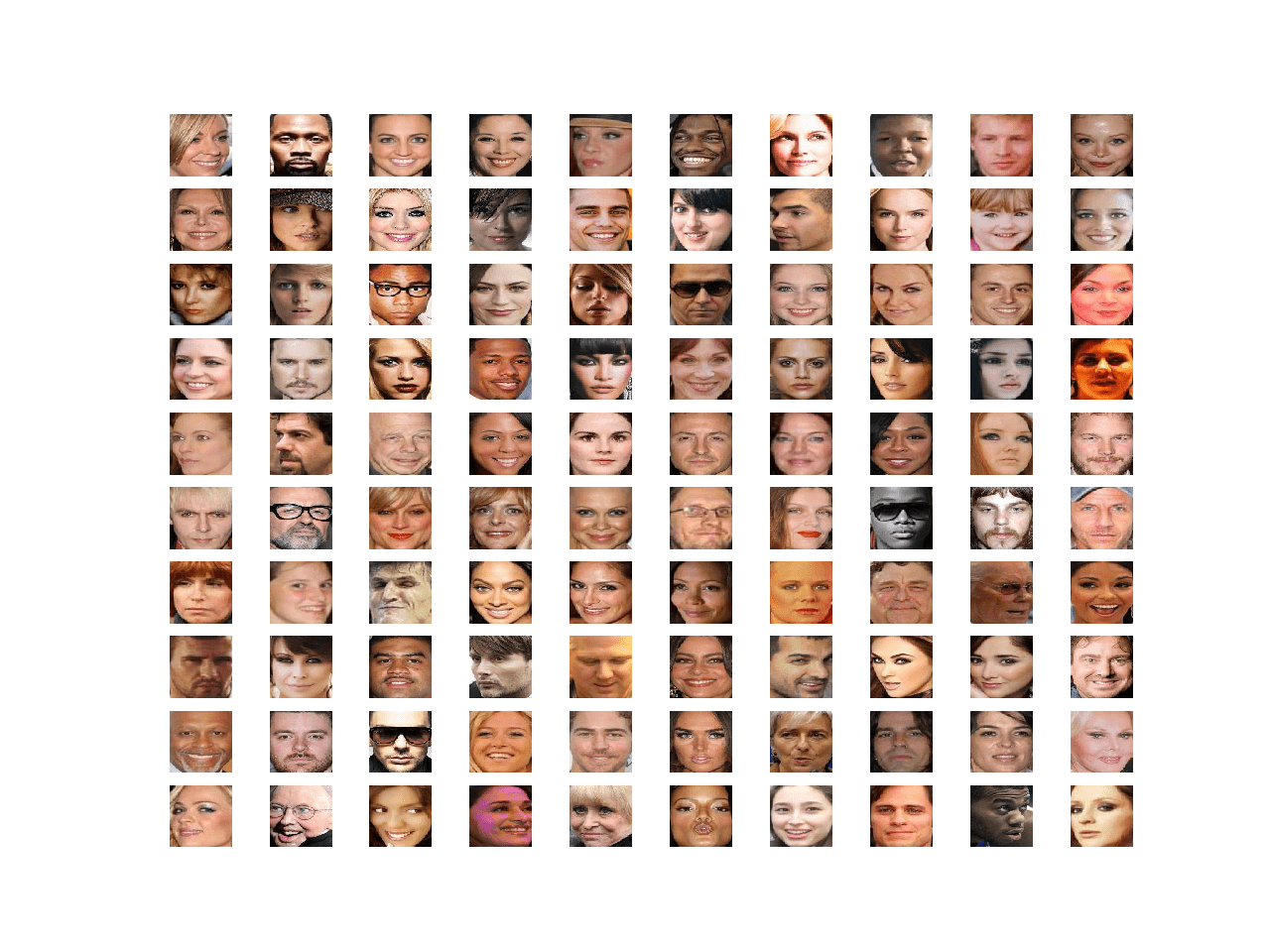
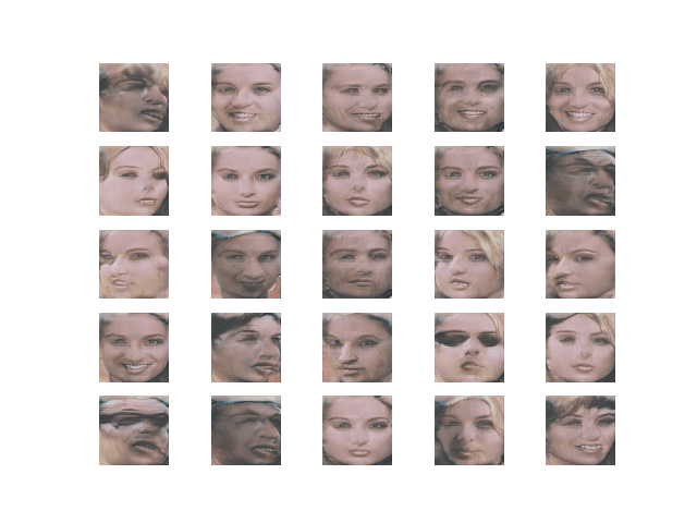
Running the example loads the dataset and creates a plot of the first 100 images.
We can see that each image only contains the face and all faces have the same square shape. Our goal is to generate new faces with the same general properties.
Plot of 100 Celebrity Faces in a 10×10 Grid
We are now ready to develop a GAN model to generate faces using this dataset.
How to Develop Progressive Growing GAN Models
There are many ways to implement the progressive growing GAN models.
In this tutorial, we will develop and implement each phase of growth as a separate Keras model and each model will share the same layers and weights.
This approach allows for the convenient training of each model, just like a normal Keras model, although it requires a slightly complicated model construction process to ensure that the layers are reused correctly.
First, we will define some custom layers required in the definition of the generator and discriminator models, then proceed to define functions to create and grow the discriminator and generator models themselves.
Progressive Growing Custom Layers
There are three custom layers required to implement the progressive growing generative adversarial network.
They are the layers:
WeightedSum: Used to control the weighted sum of the old and new layers during a growth phase.
MinibatchStdev: Used to summarize statistics for a batch of images in the discriminator.
PixelNormalization: Used to normalize activation maps in the generator model.
Additionally, a weight constraint is used in the paper referred to as “equalized learning rate“. This too would need to be implemented as a custom layer. In the interest of brevity, we won’t use equalized learning rate in this tutorial and instead we use a simple max norm weight constraint.
WeightedSum Layer
The WeightedSum layer is a merge layer that combines the activations from two input layers, such as two input paths in a discriminator or two output paths in a generator model. It uses a variable called alpha that controls how much to weight the first and second inputs.
It is used during the growth phase of training when the model is in transition from one image size to a new image size with double the width and height (quadruple the area), such as from 4×4 to 8×8 pixels.
During the growth phase, the alpha parameter is linearly scaled from 0.0 at the beginning to 1.0 at the end, allowing the output of the layer to transition from giving full weight to the old layers to giving full weight to the new layers (second input).
The mini-batch standard deviation layer, or MinibatchStdev, is only used in the output block of the discriminator layer.
The objective of the layer is to provide a statistical summary of the batch of activations. The discriminator can then learn to better detect batches of fake samples from batches of real samples. This, in turn, encourages the generator that is trained via the discriminator to create batches of samples with realistic batch statistics.
It is implemented as calculating the standard deviation for each pixel value in the activation maps across the batch, calculating the average of this value, and then creating a new activation map (one channel) that is appended to the list of activation maps provided as input.
The MinibatchStdev layer is defined below.
1
2
3
4
5
6
7
8
9
10
11
12
13
14
15
16
17
18
19
20
21
22
23
24
25
26
27
28
29
30
31
32
33
34
35
# mini-batch standard deviation layer
classMinibatchStdev(Layer):
# initialize the layer
def __init__(self,**kwargs):
super(MinibatchStdev,self).__init__(**kwargs)
# perform the operation
def call(self,inputs):
# calculate the mean value for each pixel across channels
mean=backend.mean(inputs,axis=0,keepdims=True)
# calculate the squared differences between pixel values and mean
squ_diffs=backend.square(inputs-mean)
# calculate the average of the squared differences (variance)
# add one to the channel dimension (assume channels-last)
input_shape[-1]+=1
# convert list to a tuple
returntuple(input_shape)
PixelNormalization
The generator and discriminator models don’t use batch normalization like other GAN models; instead, each pixel in the activation maps is normalized to unit length.
This is a variation of local response normalization and is referred to in the paper as pixelwise feature vector normalization. Also, unlike other GAN models, normalization is only used in the generator model, not the discriminator.
This is a type of activity regularization and could be implemented as an activity constraint, although it is easily implemented as a new layer that scales the activations of the prior layer.
The PixelNormalization class below implements this and can be used after each Convolution layer in the generator, but before any activation function.
# calculate the sqrt of the mean squared value (L2 norm)
l2=backend.sqrt(mean_values)
# normalize values by the l2 norm
normalized=inputs/l2
returnnormalized
# define the output shape of the layer
def compute_output_shape(self,input_shape):
returninput_shape
We now have all of the custom layers required and can define our models.
Progressive Growing Discriminator Model
The discriminator model is defined as a deep convolutional neural network that expects a 4×4 color image as input and predicts whether it is real or fake.
The first hidden layer is a 1×1 convolutional layer. The output block involves a MinibatchStdev, 3×3, and 4×4 convolutional layers, and a fully connected layer that outputs a prediction. Leaky ReLU activation functions are used after all layers and the output layers use a linear activation function.
This model is trained for normal interval then the model undergoes a growth phase to 8×8. This involves adding a block of two 3×3 convolutional layers and an average pooling downsample layer. The input image passes through the new block with a new 1×1 convolutional hidden layer. The input image is also passed through a downsample layer and through the old 1×1 convolutional hidden layer. The output of the old 1×1 convolution layer and the new block are then combined via a WeightedSum layer.
After an interval of training transitioning the WeightedSum’s alpha parameter from 0.0 (all old) to 1.0 (all new), another training phase is run to tune the new model with the old layer and pathway removed.
This process repeats until the desired image size is met, in our case, 128×128 pixel images.
We can achieve this with two functions: the define_discriminator() function that defines the base model that accepts 4×4 images and the add_discriminator_block() function that takes a model and creates a growth version of the model with two pathways and the WeightedSum and a second version of the model with the same layers/weights but without the old 1×1 layer and WeightedSum layers. The define_discriminator() function can then call the add_discriminator_block() function as many times as is needed to create the models up to the desired level of growth.
All layers are initialized with small Gaussian random numbers with a standard deviation of 0.02, which is common for GAN models. A maxnorm weight constraint is used with a value of 1.0, instead of the more elaborate ‘equalized learning rate‘ weight constraint used in the paper.
The paper defines a number of filters that increases with the depth of the model from 16 to 32, 64, all the way up to 512. This requires projection of the number of feature maps during the growth phase so that the weighted sum can be calculated correctly. To avoid this complication, we fix the number of filters to be the same in all layers.
Each model is compiled and will be fit. In this case, we will use Wasserstein loss (or WGAN loss) and the Adam version of stochastic gradient descent configured as is specified in the paper. The authors of the paper recommend exploring using both WGAN-GP loss and least squares loss and found that the former performed slightly better. Nevertheless, we will use Wasserstein loss as it greatly simplifies the implementation.
First, we must define the loss function as the average predicted value multiplied by the target value. The target value will be 1 for real images and -1 for fake images. This means that weight updates will seek to increase the divide between real and fake images.
1
2
3
# calculate wasserstein loss
def wasserstein_loss(y_true,y_pred):
returnbackend.mean(y_true *y_pred)
The functions for defining and creating the growth versions of the discriminator models are listed below.
We make careful use of the functional API and knowledge of the model structure to create the two models for each growth phase. The growth phase also always doubles the expected input shape.
The define_discriminator() function is called by specifying the number of blocks to create.
We will create 6 blocks, which will create 6 pairs of models that expect the input image sizes of 4×4, 8×8, 16×16, 32×32, 64×64, 128×128.
The function returns a list where each element in the list contains two models. The first model is the ‘normal model‘ or straight through model, and the second is the version of the model that includes the old 1×1 and new block with the weighted sum, used for the transition or growth phase of training.
Progressive Growing Generator Model
The generator model takes a random point from the latent space as input and generates a synthetic image.
The generator models are defined in the same way as the discriminator models.
Specifically, a base model for generating 4×4 images is defined and growth versions of the model are created for the large image output size.
The main difference is that during the growth phase, the output of the model is the output of the WeightedSum layer. The growth phase version of the model involves first adding a nearest neighbor upsampling layer; this is then connected to the new block with the new output layer and to the old old output layer. The old and new output layers are then combined via a WeightedSum output layer.
The base model has an input block defined with a fully connected layer with a sufficient number of activations to create a given number of 4×4 feature maps. This is followed by 4×4 and 3×3 convolution layers and a 1×1 output layer that generates color images. New blocks are added with an upsample layer and two 3×3 convolutional layers.
The LeakyReLU activation function is used and the PixelNormalization layer is used after each convolutional layer. A linear activation function is used in the output layer, instead of the more common tanh function, yet real images are still scaled to the range [-1,1], which is common for most GAN models.
The paper defines the number of feature maps decreasing with the depth of the model from 512 to 16. As with the discriminator, the difference in the number of feature maps across blocks introduces a challenge for the WeightedSum, so for simplicity, we fix all layers to have the same number of filters.
Also like the discriminator model, weights are initialized with Gaussian random numbers with a standard deviation of 0.02 and the maxnorm weight constraint is used with a value of 1.0, instead of the equalized learning rate weight constraint used in the paper.
The functions for defining and growing the generator models are defined below.
Calling the define_generator() function requires that the size of the latent space be defined.
Like the discriminator, we will set the n_blocks argument to 6 to create six pairs of models.
The function returns a list of models where each item in the list contains the normal or straight-through version of each generator and the growth version for phasing in the new block at the larger output image size.
Composite Models for Training the Generators
The generator models are not compiled as they are not trained directly.
Instead, the generator models are trained via the discriminator models using Wasserstein loss.
This involves presenting generated images to the discriminator as real images and calculating the loss that is then used to update the generator models.
A given generator model must be paired with a given discriminator model both in terms of the same image size (e.g. 4×4 or 8×8) and in terms of the same phase of training, such as growth phase (introducing the new block) or fine-tuning phase (normal or straight-through).
We can achieve this by creating a new model for each pair of models that stacks the generator on top of the discriminator so that the synthetic image feeds directly into the discriminator model to be deemed real or fake. This composite model can then be used to train the generator via the discriminator and the weights of the discriminator can be marked as not trainable (only in this model) to ensure they are not changed during this misleading process.
As such, we can create pairs of composite models, e.g. six pairs for the six levels of image growth, where each pair is comprised of a composite model for the normal or straight-through model, and the growth version of the model.
The define_composite() function implements this and is defined below.
1
2
3
4
5
6
7
8
9
10
11
12
13
14
15
16
17
18
19
20
21
# define composite models for training generators via discriminators
Now that we have seen how to define the generator and discriminator models, let’s look at how we can fit these models on the celebrity faces dataset.
How to Train Progressive Growing GAN Models
First, we need to define some convenience functions for working with samples of data.
The load_real_samples() function below loads our prepared celebrity faces dataset, then converts the pixels to floating point values and scales them to the range [-1,1], common to most GAN implementations.
1
2
3
4
5
6
7
8
9
10
11
# load dataset
def load_real_samples(filename):
# load dataset
data=load(filename)
# extract numpy array
X=data['arr_0']
# convert from ints to floats
X=X.astype('float32')
# scale from [0,255] to [-1,1]
X=(X-127.5)/127.5
returnX
Next, we need to be able to retrieve a random sample of images used to update the discriminator.
The generate_real_samples() function below implements this, returning a random sample of images from the loaded dataset and their corresponding target value of class=1 to indicate that the images are real.
1
2
3
4
5
6
7
8
9
# select real samples
def generate_real_samples(dataset,n_samples):
# choose random instances
ix=randint(0,dataset.shape[0],n_samples)
# select images
X=dataset[ix]
# generate class labels
y=ones((n_samples,1))
returnX,y
Next, we need a sample of latent points used to create synthetic images with the generator model.
The generate_latent_points() function below implements this, returning a batch of latent points with the required dimensionality.
1
2
3
4
5
6
7
# generate points in latent space as input for the generator
def generate_latent_points(latent_dim,n_samples):
# generate points in the latent space
x_input=randn(latent_dim *n_samples)
# reshape into a batch of inputs for the network
x_input=x_input.reshape(n_samples,latent_dim)
returnx_input
The latent points can be used as input to the generator to create a batch of synthetic images.
This is required to update the discriminator model. It is also required to update the generator model via the discriminator model with the composite models defined in the previous section.
The generate_fake_samples() function below takes a generator model and generates and returns a batch of synthetic images and the corresponding target for the discriminator of class=-1 to indicate that the images are fake. The generate_latent_points() function is called to create the required batch worth of random latent points.
1
2
3
4
5
6
7
8
9
# use the generator to generate n fake examples, with class labels
Training the models occurs in two phases: a fade-in phase that involves the transition from a lower-resolution to a higher-resolution image, and the normal phase that involves the fine-tuning of the models at a given higher resolution image.
During the phase-in, the alpha value of the WeightedSum layers in the discriminator and generator model at a given level requires linear transition from 0.0 to 1.0 based on the training step. The update_fadein() function below implements this; given a list of models (such as the generator, discriminator, and composite model), the function locates the WeightedSum layer in each and sets the value for the alpha attribute based on the current training step number.
Importantly, this alpha attribute is not a constant but is instead defined as a changeable variable in the WeightedSum class and whose value can be changed using the Keras backend set_value() function.
This is a clumsy but effective approach to changing the alpha values. Perhaps a cleaner implementation would involve a Keras Callback and is left as an exercise for the reader.
1
2
3
4
5
6
7
8
9
# update the alpha value on each instance of WeightedSum
def update_fadein(models,step,n_steps):
# calculate current alpha (linear from 0 to 1)
alpha=step/float(n_steps-1)
# update the alpha for each model
formodel inmodels:
forlayer inmodel.layers:
ifisinstance(layer,WeightedSum):
backend.set_value(layer.alpha,alpha)
Next, we can define the procedure for training the models for a given training phase.
A training phase takes one generator, discriminator, and composite model and updates them on the dataset for a given number of training epochs. The training phase may be a fade-in transition to a higher resolution, in which case the update_fadein() must be called each iteration, or it may be a normal tuning training phase, in which case there are no WeightedSum layers present.
The train_epochs() function below implements the training of the discriminator and generator models for a single training phase.
A single training iteration involves first selecting a half batch of real images from the dataset and generating a half batch of fake images from the current state of the generator model. These samples are then used to update the discriminator model.
Next, the generator model is updated via the discriminator with the composite model, indicating that the generated images are, in fact, real, and updating generator weights in an effort to better fool the discriminator.
A summary of model performance is printed at the end of each training iteration, summarizing the loss of the discriminator on the real (d1) and fake (d2) images and the loss of the generator (g).
Next, we need to call the train_epochs() function for each training phase.
This involves first scaling the training dataset to the required pixel dimensions, such as 4×4 or 8×8. The scale_dataset() function below implements this, taking the dataset and returning a scaled version.
These scaled versions of the dataset could be pre-computed and loaded instead of re-scaled on each run. This might be a nice extension if you intend to run the example many times.
1
2
3
4
5
6
7
8
9
# scale images to preferred size
def scale_dataset(images,new_shape):
images_list=list()
forimage inimages:
# resize with nearest neighbor interpolation
new_image=resize(image,new_shape,0)
# store
images_list.append(new_image)
returnasarray(images_list)
After each training run, we also need to save a plot of generated images and the current state of the generator model.
This is useful so that at the end of the run we can see the progression of the capability and quality of the model, and load and use a generator model at any point during the training process. A generator model could be used to create ad hoc images, or used as the starting point for continued training.
The summarize_performance() function below implements this, given a status string such as “faded” or “tuned“, a generator model, and the size of the latent space. The function will proceed to create a unique name for the state of the system using the “status” string such as “04×04-faded“, then create a plot of 25 generated images and save the plot and the generator model to file using the defined name.
1
2
3
4
5
6
7
8
9
10
11
12
13
14
15
16
17
18
19
20
21
22
23
# generate samples and save as a plot and save the model
The train() function below pulls this together, taking the lists of defined models as input as well as the list of batch sizes and the number of training epochs for the normal and fade-in phases at each level of growth for the model.
The first generator and discriminator model for 4×4 images are fit by calling train_epochs() and saved by calling summarize_performance().
Then the steps of growth are enumerated, involving first scaling the image dataset to the preferred size, training and saving the fade-in model for the new image size, then training and saving the normal or fine-tuned model for the new image size.
We can then define the configuration, models, and call train() to start the training process.
The paper recommends using a batch size of 16 for images sized between 4×4 and 128×128 before reducing the size. It also recommends training each phase for about 800K images. The paper also recommends a latent space of 512 dimensions.
The models are defined with six levels of growth to meet the 128×128 pixel size of our dataset. We also shrink the latent space accordingly to 100 dimensions.
Instead of keeping the batch size and number of epochs constant, we vary it to speed up the training process, using larger batch sizes for early training phases and smaller batch sizes for later training phases for fine-tuning and stability. Additionally, fewer training epochs are used for the smaller models and more epochs for the larger models.
The choice of batch sizes and training epochs is somewhat arbitrary and you may want to experiment with different values and review their effects.
1
2
3
4
5
6
7
8
9
10
11
12
13
14
15
16
17
18
# number of growth phases, e.g. 6 == [4, 8, 16, 32, 64, 128]
Running the example may take a number of hours to complete on modern GPU hardware.
Note: Your results may vary given the stochastic nature of the algorithm or evaluation procedure, or differences in numerical precision. Consider running the example a few times and compare the average outcome.
If loss values during the training iterations go to zero or very large/small numbers, this may be an example of a failure mode and may require a restart of the training process.
Running the example first reports the successful loading of the prepared dataset and the scaling of the dataset to the first image size, then reports the loss of each model for each step of the training process.
1
2
3
4
5
6
7
8
Loaded (50000, 128, 128, 3)
Scaled Data (50000, 4, 4, 3)
>1, d1=0.993, d2=0.001 g=0.951
>2, d1=0.861, d2=0.118 g=0.982
>3, d1=0.829, d2=0.126 g=0.875
>4, d1=0.774, d2=0.202 g=0.912
>5, d1=0.687, d2=0.035 g=0.911
...
Plots of generated images and the generator model are saved after each fade-in training phase with filenames like:
plot_008x008-faded.png
model_008x008-faded.h5
Plots and models are also saved after each tuning phase, with filenames like:
plot_008x008-tuned.png
model_008x008-tuned.h5
Reviewing plots of the generated images at each point helps to see the progression both in the size of supported images and their quality before and after the tuning phase.
For example, below is a sample of images generated after the first 4×4 training phase (plot_004x004-tuned.png). At this point, we cannot see much at all.
Synthetic Celebrity Faces at 4×4 Resolution Generated by the Progressive Growing GAN
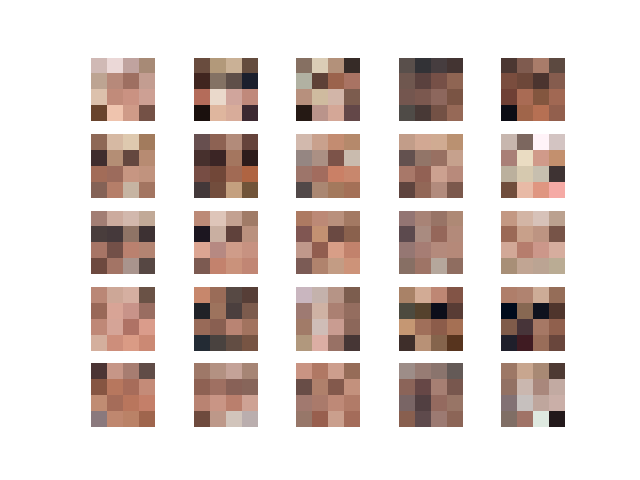
Reviewing generated images after the fade-in training phase for 8×8 images shows more structure (plot_008x008-faded.png). The images are blocky but we can see faces.
Synthetic Celebrity Faces at 8×8 Resolution After Fade-In Generated by the Progressive Growing GAN
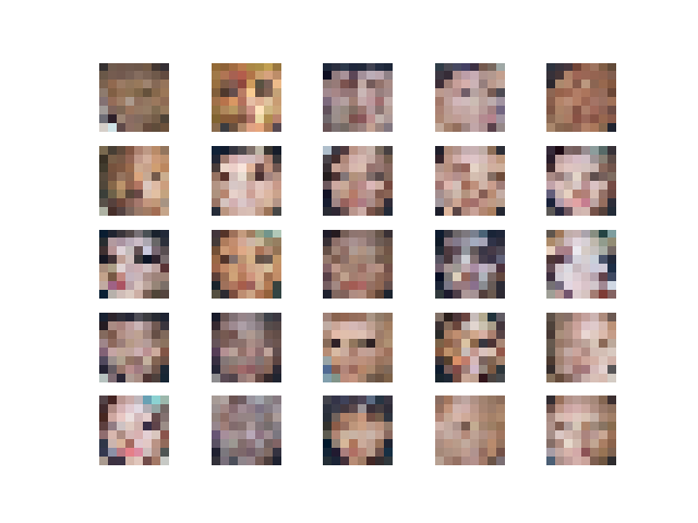
Next, we can contrast the generated images for 16×16 after the fade-in training phase (plot_016x016-faded.png) and after the tuning training phase (plot_016x016-tuned.png).
We can see that the images are clearly faces and we can see that the fine-tuning phase appears to improve the coloring or tone of the faces and perhaps the structure.
Synthetic Celebrity Faces at 16×16 Resolution After Fade-In Generated by the Progressive Growing GAN
Synthetic Celebrity Faces at 16×16 Resolution After Tuning Generated by the Progressive Growing GAN
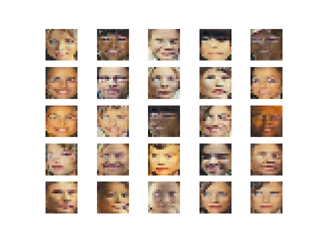
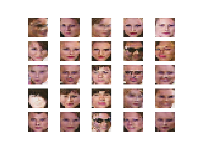
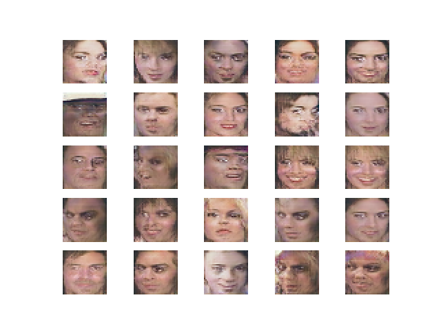
Finally, we can review generated faces after tuning for the remaining 32×32, 64×64, and 128×128 resolutions. We can see that each step in resolution, the image quality is improved, allowing the model to fill in more structure and detail.
Although not perfect, the generated images show that the progressive growing GAN is capable of not only generating plausible human faces at different resolutions, but it is able to scale building upon what was learned at lower resolutions to generate plausible faces at higher resolutions.
Synthetic Celebrity Faces at 32×32 Resolution After Tuning Generated by the Progressive Growing GAN
Synthetic Celebrity Faces at 64×64 Resolution After Tuning Generated by the Progressive Growing GAN
Synthetic Celebrity Faces at 128×128 Resolution After Tuning Generated by the Progressive Growing GAN
Now that we have seen how the generator models can be fit, next we can see how we might load and use a saved generator model.
How to Synthesize Images With a Progressive Growing GAN Model
In this section, we will explore how to load a generator model and use it to generate synthetic images on demand.
Because the generator models use custom layers, we must specify how to load the custom layers. This is achieved by providing a dict to the load_model() function that maps each of the custom layer names to the appropriate class.
Tying this together, the complete example of loading a saved progressive growing GAN generator model and using it to generate new faces is listed below.
In this case, we demonstrate loading the tuned model for generating 16×16 faces.
1
2
3
4
5
6
7
8
9
10
11
12
13
14
15
16
17
18
19
20
21
22
23
24
25
26
27
28
29
30
31
32
33
34
35
36
37
38
39
40
41
42
43
44
45
46
47
48
49
50
51
52
53
54
55
56
57
58
59
60
61
62
63
64
65
66
67
68
69
70
71
72
73
74
75
76
77
78
79
80
81
82
83
84
85
86
87
88
89
90
91
92
93
94
95
96
97
98
99
100
101
102
103
104
105
106
107
108
109
110
111
112
113
114
115
116
117
118
119
120
121
122
# example of loading the generator model and generating images
Running the example loads the model and generates 25 faces that are plotted in a 5×5 grid.
Note: Your results may vary given the stochastic nature of the algorithm or evaluation procedure, or differences in numerical precision. Consider running the example a few times and compare the average outcome.
Plot of 25 Synthetic Faces with 16×16 Resolution Generated With a Final Progressive Growing GAN Model
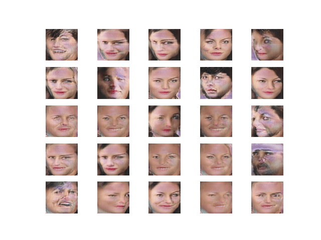
We can then change the filename to a different model, such as the tuned model for generating 128×128 faces.
1
2
...
model=load_model('model_128x128-tuned.h5',cust)
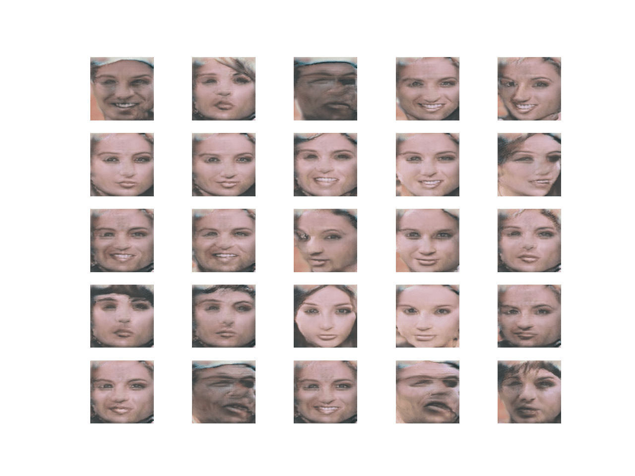
Re-running the example generates a plot of higher-resolution synthetic faces.
Plot of 25 Synthetic Faces With 128×128 Resolution Generated With a Final Progressive Growing GAN Model
Extensions
This section lists some ideas for extending the tutorial that you may wish to explore.
Change Alpha via Callback. Update the example to use a Keras callback to update the alpha value for the WeightedSum layers during fade-in training.
Pre-Scale Dataset. Update the example to pre-scale each dataset and save each version to file to be loaded when needed during training.
Equalized Learning Rate. Update the example to implement the equalized learning rate weight scaling method described in the paper.
Progression in Number of Filters. Update the example to decrease the number of filters with depth in the generator and increase the number of filters with depth in the discriminator to match the configuration in the paper.
Larger Image Size. Update the example to generate large image sizes, such as 512×512.
If you explore any of these extensions, I’d love to know.
Post your findings in the comments below.
Further Reading
This section provides more resources on the topic if you are looking to go deeper.
Please show us the code snippet for saving the data to a class specific folder, here the faces folder, for at least one of your examples. This helps us generate synthetic data for our custom data sets. Thanks in advance.
Hello, I’ve met an issue
While I ran on
”’
# directory that contains all images
directory = ‘img_align_celeba/’
# load and extract all faces
all_faces = load_faces(directory, 50000)
”’
It shows
‘AttributeError: module ‘tensorflow’ has no attribute ‘ConfigProto’ ‘
TF 2.0 got rid of tf.ConfigProto(). Use TensorFlow 1.14 as your backend and it’ll work.
Apparently you can do tf.compat.v1.ConfigProto() but I would recommend against this because you’ll run into a lot more errors anyway. Just create a virtual environment with 1.14 and it’ll work!
Thanks for this awesome tutorial! It is really helpful since I got most of the theory from your GAN book but this code is a sweet bonus.
The model mentioned here is able to generate good quality faces till 64×64, however it falls into mode collapse at 128×128 training as the generated faces look quite similar. Not a major issue as I believe this can be sorted out with some experimentation.
One thing I noticed was the discriminator and the generator loss which remains in the range of 1 to -1 in the initial epochs but after that it explodes to huge numbers but the model is still able to generate some natural looking faces:
couple of lines from training log
>9273, d1=-7246121533440.000, d2=8692378370048.000 g=-1543880310784.000
>9274, d1=-10451597393920.000, d2=2355663208448.000 g=1763277799424.000
I tried increasing the latent dimension and reducing the learning rate but the behavior remains the same. Any idea what might be causing this?
Hmmm, I was not happy with this example. It works, but its not great.
I think it could be improved a lot by adding the regularization technique described in the paper. I in fact tried it and it was effective, but too complicated for the tutorial.
1. You say “I think it could be improved a lot by adding the regularization technique described in the paper. I in fact tried it and it was effective, but too complicated for the tutorial.”
Would you please list the techniques that you have not yet applied in your tutorial? I see “MinibatchStdev” and “PixelNormalization”. What techniques are missing?
2. The original paper seems to suggest use of He’s “kernel_initializer” but you use RandomNormal(stddev=0.02). Can please explain the choice?
Same problem of Manjeet for me:
>67000, d1=9151679823872.000, d2=14003751354368.000 g=-61246267195392.000
>67500, d1=-84513548952141824.00, d2=59292667766374400.00 g=-25230321523884032.
>68000, d1=-511915038081024.000, d2=908596707590144.000 g=31027279953920.000
>68500, d1=nan, d2=nan g=nan
>69000, d1=nan, d2=nan g=nan
…
I still like the example because it brings us to the next level. There is always a reward that we get, after completing these tutorials. We are never left empty hands by Jason. It can be a digit classifier, may be a tool identifying cats and dogs, or other fun stuff. The student are always receiving a gift at the end of their effort and this is very motivating. It helps to keep on when it is though. I was wondering, however, if persisting with the hard work, we were going to get beyond the toy. Here we are, it is for real now, we can touch the challenge and obtain the reward of grown up kids. Let’s face it, we need to load at once 50K colored images of size 128×128. We can see that sys.getsizeof(np.ones((50000,128,128,3))) = 19.6 GBytes. Not for tender machines (I immediately killed mine). We could load smaller batches, but compromise on performances, GANs require some efficiency; this is the business, if we want to start playing with the professional. So, all the ancillary needs to be worked out, AWS, CGC, etc. Then, after the environment is ready, we need to put all the GAN concepts together and make it work. Following this example, all the pieces fit, we do create faces at the end. It is a little sketchy, it burned out my trial google account, but it is faces what comes out of there; faces from latent points. It is not a trivial cut and paste from a repository of eyes, mouths and noses, combining them together, it is the creation from scratch of all these elements and verification that they match alone and together our idea of a human face. Isn’t that magic? These examples are demanding, but they prove us how far we can get, working through these tutorials. Thank you Jason!
Yes, it is impressive technology, but these examples start reaching the limit of hobby and require large machines that run at some expense.
I worked on this example for a few weeks and it cost me a few thousand dollars in EC2 time, and still my results did not reach those of the paper. It’s hard work.
You just wrote that you tried to implement the regularization techniques described in the paper and that it was just too difficult for this tutorial. Since I am a complete novice in GAN programming, I would be very happy if you would share the code anyway.
I also wondered if line 410 should not be:
summarize_performance(‘faded’, g_fadein, latent_dim)
Amazing tutorial, I definitely learned a lot.
The performance for me was very poor – it might be because I only used 5k samples due to GPU constraints. Overall not a great performance, but I learned a lot! — thank you!!!!!
I wanted to ask you if you could do a tutorial for BigGAN on some face generating tasks?
Also, another question I had was if you could cover the topics of Data Preparation in-depth, by this I mean showing how to prepare data from an imported library from Keras or just downloading the data?
Lastly, I wanted to ask you if you could do a tutorial with taking a pre-trained network (like VGG16) and using its conv_base only and then training it on your own data set (eg. dogs vs cats)? I can’t seem to get my network to train — might be because I don’t understand how to prepare data properly.
Overall,
Thank you for all you do, you have helped me a lot.
Best wishes
Thanks for the great post. I am trying to change the code to work for grey scale image, i.e., (N, N, 1) rather than (N, N, 3). I think I should change input_shape=(4,4,3) to (4,4,1) in define_discriminator. I also think I should probably change n_input_layers=3 to 1 in add_discriminator_block. Are there any other changes that I have make? Thank you.
Hi Jason, many thanks for your great tutorial.
If you don’t copy weights from trained smaller model to larger model, there is no need to train smaller models. Directly training final largest model could have the same results. Am I right?
Thanks for the great tutorial. I was unhappy with the results of my GAN and a colleague recommended to try a PGAN. (Shoulder-up profiles of people, it can’t learn faces)
Your results are really nice and I saw your comment about spending a lot on EC2 for this. Did you use the [5, 8, 8, 10, 10, 10] for your epochs or was it more, and if so, what was it?
Also, does batch size affect it too much depending on stage? My 980Ti can handle batch size 64 with 8,000 images so I’ve been using that on the GAN. Should I use that at every stage of the PGAN, or is there a rule of thumb for scaling batch size throughout the process?
First of all, thanks a lot for this amazing tutorial. Every tutorial you make brings us to the next step of our learning process.
I have a question though, why the learning rate is kept so small ? A batch size of 256 or 512 could easily fit in VRAM, why don’t we do that (assuming we would also crank up the learning rate, by a factor of k or sqrt(k) assuming new_batch_size/old_batch_size = k) ?
Hi Jason,
I am trying to implement a progressive growing GAN following your example. Could you please tell me why when growing the network we take the layer previous to the last one? The one indexed with old_model.layers[-2].output . This will be very helpful to me. Moreover, is it right to say that we upsample the layer in order for it to match the size of the new grown output model? so, in this way, we can perform the weighted sum of the two outputs.
Dear Jason,
thanks for your reply; however, I am getting a loss which is really and astoundingly big! like -487258742855746.00 or the equivalent but positive, is it normal?
Today I will debug and try to figure it out, but in the meantime i got also ‘nan’ from loss computation.
Hi Jason,
if I at some point need to stop the training and then want to restart it, how would I solve this?
So I have my models saved as:
model_004x004-tuned.h5
model_008x008-faded.h5
…
and so on, and need to arrange them into the d_models and g_models lists so that I can call: gan_models = define_composite(d_models, g_models)
I use the keras method load_model to import my models.
I’m stuck on how to put them into the d_models and g_models list.
Could you help me with this? Thanks!
hi!
Thankyou for this great tutorial. i was wondering if you could explain how can i calculate fid score between these real and synthetic datasets with 10000 random images of both datasets. Moreover, is it possible to use conditional generation on top of this trained model. if yes, then how could i explore the latent space and create conditional images.
I implemented least square as loss function and trained model for specified epochs still it was not able to predict expected images. And the loss increased to very high value up to 1e+7. So is their any other way of making it better ?
Hi
Thank you for this great tutorial. Can we generate 1024*1024 or 2048*2048 image using Progressive Growing GAN ? If not, then which GAN is good for generate 1024*1024 or 2048*2048 high quality images?
Hi
Great article, thanks for that!
I’m trying to implement it and add equalized learning rates. If I understand correctly, this should be easy: I’m calculating value and on every call of Conv2D layer I’m multiplying weights of it by this scale:
Hey Jason,
This was a great article! I am trying to implement a variation of this model by adding conditioning data(text embeddings). So I modified the generator to have multiple inputs. But the Sequential API doesn’t allow us to use multiple inputs and that makes it tough to build the composite model. Is there any other way to work on this? Or should I make use of the Model subclassing API?
Thanks for the great tutorial. I applied the code to generate large medical images. However, loss value becomes a very large number when it reaches the 32 by 32 resolution. Is there a way to avoid this? I tried decreasing the learning rate but it did not help.
A big thanks to you sir for this exploratory tutorial. I have executed around all of the segments individually till dataset preperation and after that a consolidated code i executed metioned in the prieous last segment and i got the following error.
in define_discriminator(n_blocks, input_shape)
182 old_model = model_list[i – 1][0]
183 # create new model for next resolution
–> 184 models = add_discriminator_block(old_model)
185 # store model
186 model_list.append(models)
in add_discriminator_block(old_model, n_input_layers)
114 in_shape = list(old_model.input.shape)
115 # define new input shape as double the size
–> 116 input_shape = (in_shape[-2].value*2, in_shape[-2].value*2, in_shape[-1].value)
117 in_image = Input(shape=input_shape)
118 # define new input processing layer
AttributeError: ‘int’ object has no attribute ‘value’
I am not getting any idea how to remove this. I am not much aware with the functionaly of it. Can you help me to get out of this error?
Great tutorial about GAN. Sir i am tryig to use for just 500 images can i know what can be batch size and epochs used for 500 images as i got error:
—————————————————————————
AttributeError Traceback (most recent call last)
in
416 latent_dim = 100
417 # define models
–> 418 d_models = define_discriminator(n_blocks)
419 # define models
420 g_models = define_generator(latent_dim, n_blocks)
in define_discriminator(n_blocks, input_shape)
181 old_model = model_list[i – 1][0]
182 # create new model for next resolution
–> 183 models = add_discriminator_block(old_model)
184 # store model
185 model_list.append(models)
in add_discriminator_block(old_model, n_input_layers)
113 in_shape = list(old_model.input.shape)
114 # define new input shape as double the size
–> 115 input_shape = (in_shape[-2].value*2, in_shape[-2].value*2, in_shape[-1].value)
116 in_image = Input(shape=input_shape)
117 # define new input processing layer
AttributeError: ‘int’ object has no attribute ‘value’
I do not know if this question is still relevant or not, but perhaps it will be useful for beginners.
I used my dataset with 1000 images and got the same error.
I fixed it by changing the code to this (in_shape[-2]*2, in_shape[-2]*2, in_shape[-1])
Using TensorFlow backend.
/usr/local/lib/python3.6/dist-packages/keras/engine/saving.py:341: UserWarning: No training configuration found in save file: the model was *not* compiled. Compile it manually.
warnings.warn(‘No training configuration found in save file: ‘
This error occurs when using the saved model to generate new images.
/usr/local/lib/python3.6/dist-packages/keras/engine/saving.py:341: UserWarning: No training configuration found in save file: the model was *not* compiled. Compile it manually.
warnings.warn(‘No training configuration found in save file: ‘
This error occurs when i use the saved model for generating images
Thanks for the great tutorial. I want to use the PGAN for generating skin lesion images which have two classes i.e. benign and malignant. When I will use the PGAN to generate more lesion images, how can I label them that which one is benign and which one is malignant as the target to use the generate data in model training to improve the model accuracy. Can you kindly tell me the approach or some of your tutorial where you share this kind of work ?
thank you very much for this tutorial. It has been very helpful in my work.
I am getting an error when I try to save the generator model in h5 format (g_model.save(filename2). The error is “TypeError: (‘Not JSON Serializable:’, )”.
Another interesting thing is that for the 4×4 model everything goes smoothly, the error pops up when the 8×8 faded model wants to be saved.
Has anyone experienced the same error? Do you have any suggestion on how to proceed?
(I tried to save just the model weights and that worked fine, but I am interested in saving the model)
I am getting the same error as you, and for me the error is generated after 8×8 faded model. I have been able to look for solutions and only commenting our the model.save function has worked for me.
If you were able to figure it out, please let me know.
Hey Jason, I have a GTX1650 GPU on my laptop do you think i’ll be able to run this code on that. If yes what do you think are some changes in batch size or learning rate that i should be making . Thanks in advance.
Thanks Jason for amazing tutorial
I tried training it for 10k images and at 64×64 tuned phase training the loss went to nan and the images produced were black images , pls suggest some way to overcome this
Also saving the model after 4×4 is not working , giving not json serializable error, might be bcoz for weighted sum layer
But saving weights is possible
Hey Jason, i’m getting this error when i’m using TPU.
Help me.
WARNING:tensorflow:7 out of the last 7 calls to <function Model.make_predict_function..predict_function at 0x7fbaa1340268> triggered tf.function retracing. Tracing is expensive and the excessive number of tracings could be due to (1) creating @tf.function repeatedly in a loop, (2) passing tensors with different shapes, (3) passing Python objects instead of tensors. For (1), please define your @tf.function outside of the loop. For (2), @tf.function has experimental_relax_shapes=True option that relaxes argument shapes that can avoid unnecessary retracing. For (3), please refer to https://www.tensorflow.org/tutorials/customization/performance#python_or_tensor_args and https://www.tensorflow.org/api_docs/python/tf/function for more details.
WARNING:tensorflow:7 out of the last 7 calls to <function Model.make_predict_function..predict_function at 0x7fbaa1340268> triggered tf.function retracing. Tracing is expensive and the excessive number of tracings could be due to (1) creating @tf.function repeatedly in a loop, (2) passing tensors with different shapes, (3) passing Python objects instead of tensors. For (1), please define your @tf.function outside of the loop. For (2), @tf.function has experimental_relax_shapes=True option that relaxes argument shapes that can avoid unnecessary retracing. For (3), please refer to https://www.tensorflow.org/tutorials/customization/performance#python_or_tensor_args and https://www.tensorflow.org/api_docs/python/tf/function for more details.
WARNING:tensorflow:8 out of the last 8 calls to <function Model.make_predict_function..predict_function at 0x7fbaa1340268> triggered tf.function retracing. Tracing is expensive and the excessive number of tracings could be due to (1) creating @tf.function repeatedly in a loop, (2) passing tensors with different shapes, (3) passing Python objects instead of tensors. For (1), please define your @tf.function outside of the loop. For (2), @tf.function has experimental_relax_shapes=True option that relaxes argument shapes that can avoid unnecessary retracing. For (3), please refer to https://www.tensorflow.org/tutorials/customization/performance#python_or_tensor_args and https://www.tensorflow.org/api_docs/python/tf/function for more details.
WARNING:tensorflow:8 out of the last 8 calls to <function Model.make_predict_function..predict_function at 0x7fbaa1340268> triggered tf.function retracing. Tracing is expensive and the excessive number of tracings could be due to (1) creating @tf.function repeatedly in a loop, (2) passing tensors with different shapes, (3) passing Python objects instead of tensors. For (1), please define your @tf.function outside of the loop. For (2), @tf.function has experimental_relax_shapes=True option that relaxes argument shapes that can avoid unnecessary retracing. For (3), please refer to https://www.tensorflow.org/tutorials/customization/performance#python_or_tensor_args and https://www.tensorflow.org/api_docs/python/tf/function for more details.
WARNING:tensorflow:9 out of the last 9 calls to <function Model.make_predict_function..predict_function at 0x7fbaa1340268> triggered tf.function retracing. Tracing is expensive and the excessive number of tracings could be due to (1) creating @tf.function repeatedly in a loop, (2) passing tensors with different shapes, (3) passing Python objects instead of tensors. For (1), please define your @tf.function outside of the loop. For (2), @tf.function has experimental_relax_shapes=True option that relaxes argument shapes that can avoid unnecessary retracing. For (3), please refer to https://www.tensorflow.org/tutorials/customization/performance#python_or_tensor_args and https://www.tensorflow.org/api_docs/python/tf/function for more details.
WARNING:tensorflow:9 out of the last 9 calls to <function Model.make_predict_function..predict_function at 0x7fbaa1340268> triggered tf.function retracing. Tracing is expensive and the excessive number of tracings could be due to (1) creating @tf.function repeatedly in a loop, (2) passing tensors with different shapes, (3) passing Python objects instead of tensors. For (1), please define your @tf.function outside of the loop. For (2), @tf.function has experimental_relax_shapes=True option that relaxes argument shapes that can avoid unnecessary retracing. For (3), please refer to https://www.tensorflow.org/tutorials/customization/performance#python_or_tensor_args and https://www.tensorflow.org/api_docs/python/tf/function for more details.
—————————————————————————
InvalidArgumentError Traceback (most recent call last)
in ()
45 with strategy.scope():
46 directory = ‘/content/img_align_celeba/img_align_celeba/’
—> 47 all_faces = load_faces(directory, 500)
48 print(‘Loaded: ‘, all_faces.shape)
49 savez_compressed(‘img_align_celeba_128.npz’, all_faces)
9 frames
/usr/local/lib/python3.6/dist-packages/tensorflow/python/eager/context.py in sync_executors(self)
656 “””
657 if self._context_handle:
–> 658 pywrap_tfe.TFE_ContextSyncExecutors(self._context_handle)
659 else:
660 raise ValueError(“Context is not initialized.”)
InvalidArgumentError: 9 root error(s) found.
(0) Invalid argument: {{function_node __inference_predict_function_22890}} Compilation failure: Dynamic Spatial Convolution is not supported: lhs shape is f32[<=2,<=54,<=66,3]
[[{{node functional_13/conv2d_24/Conv2D}}]]
TPU compilation failed
[[tpu_compile_succeeded_assert/_1842486143609259834/_4]]
[[cluster_predict_function/control_after/_1/_287]]
(1) Invalid argument: {{function_node __inference_predict_function_22890}} Compilation failure: Dynamic Spatial Convolution is not supported: lhs shape is f32[<=2,<=54,<=66,3]
[[{{node functional_13/conv2d_24/Conv2D}}]]
TPU compilation failed
[[tpu_compile_succeeded_assert/_1842486143609259834/_4]]
[[cluster_predict_function/control_after/_1/_283]]
(2) Invalid argument: {{function_node __inference_predict_function_22890}} Compilation failure: Dynamic Spatial Convolution is not supported: lhs shape is f32[<=2,<=54,<=66,3]
[[{{node functional_13/conv2d_24/Conv2D}}]]
TPU compilation failed
[[tpu_compile_succeeded_assert/_1842486143609259834/_4]]
[[cluster_predict_function/control_after/_1/_275]]
(3) Invalid argument: {{function_node __inference_predict_function_22890}} Compilation failure: Dynamic Spatial Convolution is not supported: lhs shape is f32[<=2,<=54,<=66,3]
[[{{node functional_13/conv2d_24/Conv2D}}]]
TPU compilation failed
[[tpu_compile_succeeded_assert/_1842486143609259834/_4]]
[[cluster_predict_function/control_after/_1/_295]]
(4) Invalid argument: {{function_node __inference_predict_function_22890}} Compilation failure: Dynamic Spatial Convolution is not supported: lhs shape is f32[<=2,<=54,<=66,3]
[[{{node functional_13/conv2d_24/Conv2D}}]]
TPU compilation failed
[[tpu_compile_succeeded_assert/_1842486143609259834/_4]]
[[cluster_predict_function/control_after/_1/_291]]
(5) Invalid argument: {{function_node __inference_predict_function_22890}} Compilation failure: Dynamic Spatial Convolution is not supported: lhs shape is f32[<=2,<=54,<=66,3]
[[{{node functional_13/conv2d_24/Conv2D}}]]
TPU compilation failed
[[tpu_compile_succeeded_assert/_1842486143609259834/_4]]
[[cluster_predict_function/control_after/_1/_279]]
(6) Invalid argument: {{function_node __inference_predict_function_22890}} Compilation failure: Dynamic Spatial Convolution is not supported: lhs shape is f32[<=2,<=54,<=66,3]
[[{{node functional_13/conv2d_24/Conv2D}}]]
TPU compilation failed
[[tpu_compile_succeeded_assert/_1842486143609259834/_4]]
[[cluster_predict_function/control_after/_1/_303]]
(7) Invalid argument: {{function_node __inference_predict_function_22890}} Compilation failure: Dynamic Spatial Convolution is not supported: lhs shape is f32[<=2,<=54,<=66,3]
[[{{node functional_13/conv2d_24/Conv2D}}]]
TPU compilation failed
[[tpu_compile_succeeded_assert/_1842486143609259834/_4]]
[[cluster_predict_function/control_after/_1/_299]]
(8) Invalid argument: {{function_node __inference_predict_function_22890}} Compilation failure: Dynamic Spatial Convolution is not supported: lhs shape is f32[ … [truncated]
“Running the example may take a few minutes given the larger number of faces to be loaded.”
Running this example with mtcnn v0.1.0 using tensorflow backend takes literally ages for me. Looking at benchmarks of mtcnn I should get a two-figure FPS number, but I can’t even reach 1 FPS. Seems odd, as I’m using RTX 3090 GPU.
I will test this implementation using the whole images, not just the faces.
It’s important for me to understand every single step of the implementation and why you’ve done it the way you did.
Your tutorials are very helpful for me and got me into machine learning in general. Thank you very much, sir.
Fantastic tutorial. This is of great help. Thanks a lot!
As I was reading about your lstm autoencoder introduction, I was wondering if there is a possibilty to combine those concepts: Something like a progressive growing lstm gan?
Thakns for this tutorial !
Your call to the train function doesnt have e_norm , e_fadein parameters which doesnt allow me to run your examples, do you have a solution?
Thanks for this tutorial,
I have a question, I want to add some changes to this code. So, when I use d_model. trainable_weights in order to calculate gradients, it returns [] value. Do you have any idea about the problem?
1. You say “I think it could be improved a lot by adding the regularization technique described in the paper. I in fact tried it and it was effective, but too complicated for the tutorial.”
Would you please list the techniques that you have not yet applied in your tutorial? I see “MinibatchStdev” and “PixelNormalization”. What techniques are missing?
2. The original paper seems to suggest use of He’s “kernel_initializer” but you use RandomNormal(stddev=0.02). Can please explain the choice?
Hi, are Progressive GAN and style GAN only effective for synthesizing high-resolution images? in case of producing low-resolution images like MNIST is there any difference in quality compared to simple GAN?
Hi, actually I think the comments are misleading. In the literature, it has a 1/N term, and your code correctly implements the root, of the mean squared, (which would be called RMS Normalization?) But the comments refer to L2_Normalization, which doesn’t have the 1/N term. L2_norm is just the sum, not the mean. If you want L2_norm you could just do: backend.l2_normalize(inputs, axis=-1)
Anyway, I mentioned the wrong module for rsqrt its from tensorflow.python.ops.math_ops, full example should be:
# perform the operation
def call(self, inputs):
# calculate square pixel values
values = inputs**2.0
# calculate the mean pixel values
mean_values = backend.mean(values, axis=-1, keepdims=True)
# ensure the mean is not zero
mean_values += 1.0e-8
# calculate the inverse square root of the mean squared value (RMS Norm)
rms = math_ops.rsqrt(mean_values)
# normalize values by the rms
normalized = inputs * rms
return normalized
I can’t get your example to work, but I think I’ve spotted a bug, you pass in [g_model, d_model, gan_model] to the update_fadein function and check whether each model.layer is an instance of WeightedSum, however gan_model is nested, it only has two layers which are the generator model, and the discriminator model. I think you have to make the call recursive if the layer is an isinstance(Model), or just pass in gan_model.layers[0], gan_model.layers[1]
I managed to fix the NaN error issue by using clipvalue=0.1 in both generator and discriminator optimizers
however, I’m not sure if this can be done, because in theory it can cause bad gradients in the generator
thank you! I would also like to ask you something . I try to create a face recogntion system in a kind of electronic glasses that works in real time ,but i have several problems such as low resolution blur of the faces etc.Do you think it is better to restore faces with GANS and then apply them in the model to take the embedings or could you suggest me a better way to do it without face restoration(for example train a FR model in low resolution dataset).I have also observed that model behaves well in Celeba dataset but in custom dataset not so much ,so is it a way to transform faces after face detection (crop and alighment) to look like Celeba data?
Your model is really impressive but I’ve spent the entire day trying to implement it and I am struggling. I managed to fix all the issues except one. When I train the model, I have a dataset as a numpy array with shape (13153, 128, 128, 3) and I converted it to npz so I could match your code. My model trains for the first scale (13153, 4, 4, 3) after 4110 steps I get the plot 004x–4 tuned png. However for (13153, 8, 8, 3), I get an error after 6576 steps, this is the error, please help I have tried everything. Please let me know if you know how to debug this, I am desperate to see the end results of this model! Thanks in advance and thanks for this post, it has been really helpful in learning about PGAN and I enjoyed it.
>6576, d1=-36738.984, d2=43196.312 g=-29011.340
1/1 [==============================] – 0s 32ms/step
WARNING:tensorflow:Compiled the loaded model, but the compiled metrics have yet to be built. model.compile_metrics will be empty until you train or evaluate the model.
>Saved: plot_008x008-faded.png and model_008x008-faded.h5
1/1 [==============================] – 0s 129ms/step
ValueError Traceback (most recent call last)
in ()
6 n_epochs = [5, 8, 8, 10, 10, 10]
7
—-> 8 history_pcgan = train(g_models, d_models, gan_models, dataset, latent_dim, n_epochs, n_epochs, n_batch)
ValueError: in user code:
File “/usr/local/lib/python3.9/dist-packages/keras/engine/training.py”, line 1249, in train_function *
return step_function(self, iterator)
File “”, line 78, in wasserstein_loss *
return backend.mean(y_true * y_pred)
ValueError: Dimensions must be equal, but are 8 and 4 for ‘{{node wasserstein_loss/mul}} = Mul[T=DT_FLOAT](IteratorGetNext:1, model_25/minibatch_stdev_3/concat)’ with input shapes: [8,1], [8,4,4,129].
——————————————————


 From Scratch with Keras")


It feels nice to see our pggan implementation in Keras being cited : ) .
Thanks.
Please show us the code snippet for saving the data to a class specific folder, here the faces folder, for at least one of your examples. This helps us generate synthetic data for our custom data sets. Thanks in advance.
If you need help saving images, perhaps this will help:
https://machinelearningmastery.com/how-to-load-convert-and-save-images-with-the-keras-api/
Can we make SRGAN (https://arxiv.org/abs/1609.04802) progressive?
Good question, I’m not sure off the cuff. Perhaps try experimenting?
Hello, I’ve met an issue
While I ran on
”’
# directory that contains all images
directory = ‘img_align_celeba/’
# load and extract all faces
all_faces = load_faces(directory, 50000)
”’
It shows
‘AttributeError: module ‘tensorflow’ has no attribute ‘ConfigProto’ ‘
I am using Tensorflow 2.0.0
Thanks.
Sorry, I have not seen that error before, and I don’t think it is related to this tutorial.
I have some suggestions here that may help:
https://machinelearningmastery.com/faq/single-faq/why-does-the-code-in-the-tutorial-not-work-for-me
TF 2.0 got rid of tf.ConfigProto(). Use TensorFlow 1.14 as your backend and it’ll work.
Apparently you can do tf.compat.v1.ConfigProto() but I would recommend against this because you’ll run into a lot more errors anyway. Just create a virtual environment with 1.14 and it’ll work!
Hi Jason,
Thanks for this awesome tutorial! It is really helpful since I got most of the theory from your GAN book but this code is a sweet bonus.
The model mentioned here is able to generate good quality faces till 64×64, however it falls into mode collapse at 128×128 training as the generated faces look quite similar. Not a major issue as I believe this can be sorted out with some experimentation.
One thing I noticed was the discriminator and the generator loss which remains in the range of 1 to -1 in the initial epochs but after that it explodes to huge numbers but the model is still able to generate some natural looking faces:
couple of lines from training log
>9273, d1=-7246121533440.000, d2=8692378370048.000 g=-1543880310784.000
>9274, d1=-10451597393920.000, d2=2355663208448.000 g=1763277799424.000
I tried increasing the latent dimension and reducing the learning rate but the behavior remains the same. Any idea what might be causing this?
Hmmm, I was not happy with this example. It works, but its not great.
I think it could be improved a lot by adding the regularization technique described in the paper. I in fact tried it and it was effective, but too complicated for the tutorial.
Hi Jason,
Two questions:
1. You say “I think it could be improved a lot by adding the regularization technique described in the paper. I in fact tried it and it was effective, but too complicated for the tutorial.”
Would you please list the techniques that you have not yet applied in your tutorial? I see “MinibatchStdev” and “PixelNormalization”. What techniques are missing?
2. The original paper seems to suggest use of He’s “kernel_initializer” but you use RandomNormal(stddev=0.02). Can please explain the choice?
Same problem of Manjeet for me:
>67000, d1=9151679823872.000, d2=14003751354368.000 g=-61246267195392.000
>67500, d1=-84513548952141824.00, d2=59292667766374400.00 g=-25230321523884032.
>68000, d1=-511915038081024.000, d2=908596707590144.000 g=31027279953920.000
>68500, d1=nan, d2=nan g=nan
>69000, d1=nan, d2=nan g=nan
…
I still like the example because it brings us to the next level. There is always a reward that we get, after completing these tutorials. We are never left empty hands by Jason. It can be a digit classifier, may be a tool identifying cats and dogs, or other fun stuff. The student are always receiving a gift at the end of their effort and this is very motivating. It helps to keep on when it is though. I was wondering, however, if persisting with the hard work, we were going to get beyond the toy. Here we are, it is for real now, we can touch the challenge and obtain the reward of grown up kids. Let’s face it, we need to load at once 50K colored images of size 128×128. We can see that sys.getsizeof(np.ones((50000,128,128,3))) = 19.6 GBytes. Not for tender machines (I immediately killed mine). We could load smaller batches, but compromise on performances, GANs require some efficiency; this is the business, if we want to start playing with the professional. So, all the ancillary needs to be worked out, AWS, CGC, etc. Then, after the environment is ready, we need to put all the GAN concepts together and make it work. Following this example, all the pieces fit, we do create faces at the end. It is a little sketchy, it burned out my trial google account, but it is faces what comes out of there; faces from latent points. It is not a trivial cut and paste from a repository of eyes, mouths and noses, combining them together, it is the creation from scratch of all these elements and verification that they match alone and together our idea of a human face. Isn’t that magic? These examples are demanding, but they prove us how far we can get, working through these tutorials. Thank you Jason!
Great comment.
Yes, it is impressive technology, but these examples start reaching the limit of hobby and require large machines that run at some expense.
I worked on this example for a few weeks and it cost me a few thousand dollars in EC2 time, and still my results did not reach those of the paper. It’s hard work.
You spent a few thousand dollars instead of just buying a GPU that costs less than that and gives you infinite time for free?? why??
Great question.
I prefer to rend GPUs just-in-time rather than to (1) own, (2) operate, and (3) maintain an additional box. The trade-off is a no brainer for me.
I don’t think that make sense.
Not at all. Depends if you value money or time.
If the example is such large and you need GPU for free than Google Colab is the best option
Thanks for the suggestion. I have never used colab, I know nothing about it.
It’s just a simple notebook with GPU as well as TPU(explicitly selecting anyone among them) power and that too for free.
Hello Jason,
really nice tutorial, thanks for that.
You just wrote that you tried to implement the regularization techniques described in the paper and that it was just too difficult for this tutorial. Since I am a complete novice in GAN programming, I would be very happy if you would share the code anyway.
I also wondered if line 410 should not be:
summarize_performance(‘faded’, g_fadein, latent_dim)
instead of:
summarize_performance(‘faded’, g_normal, latent_dim).
Many thanks and best wishes
Yes, I think you’re right. Fixed.
I may share it in the future. For now, perhaps check some of the links to related projects at the end of the post for different implementations?
Hey Jason,
Amazing tutorial, I definitely learned a lot.
The performance for me was very poor – it might be because I only used 5k samples due to GPU constraints. Overall not a great performance, but I learned a lot! — thank you!!!!!
I wanted to ask you if you could do a tutorial for BigGAN on some face generating tasks?
Also, another question I had was if you could cover the topics of Data Preparation in-depth, by this I mean showing how to prepare data from an imported library from Keras or just downloading the data?
Lastly, I wanted to ask you if you could do a tutorial with taking a pre-trained network (like VGG16) and using its conv_base only and then training it on your own data set (eg. dogs vs cats)? I can’t seem to get my network to train — might be because I don’t understand how to prepare data properly.
Overall,
Thank you for all you do, you have helped me a lot.
Best wishes
Thanks!
Yes, it’s not an efficient implementation.
Great suggestion, thanks!
Yes, I have many tutorials on loading and scaling image data. Start here:
https://machinelearningmastery.com/how-to-manually-scale-image-pixel-data-for-deep-learning/
Yes, I have tons of tutorials on transfer learning as well. Start here:
https://machinelearningmastery.com/how-to-develop-a-convolutional-neural-network-to-classify-photos-of-dogs-and-cats/
Thank you very much!!
I am very grateful for your help and truly appreciate it.
Best wishes
You’re welcome.
Thanks for the great post. I am trying to change the code to work for grey scale image, i.e., (N, N, 1) rather than (N, N, 3). I think I should change input_shape=(4,4,3) to (4,4,1) in define_discriminator. I also think I should probably change n_input_layers=3 to 1 in add_discriminator_block. Are there any other changes that I have make? Thank you.
That looks like a good start.
Let me know how you go!
n_input_layers should remain set 3 only
I have one doubt, In this tutorial I can’t find the code that you have used for copying weights from trained smaller model to larger model
We don’t copy weights, we simply add more layers to existing layers/models.
Hi Jason, many thanks for your great tutorial.
If you don’t copy weights from trained smaller model to larger model, there is no need to train smaller models. Directly training final largest model could have the same results. Am I right?
No.
The idea is that we keep the weights from the smaller models and it makes learning the larger models easier.
Hey Jason,
Thanks for the great tutorial. I was unhappy with the results of my GAN and a colleague recommended to try a PGAN. (Shoulder-up profiles of people, it can’t learn faces)
Your results are really nice and I saw your comment about spending a lot on EC2 for this. Did you use the [5, 8, 8, 10, 10, 10] for your epochs or was it more, and if so, what was it?
Also, does batch size affect it too much depending on stage? My 980Ti can handle batch size 64 with 8,000 images so I’ve been using that on the GAN. Should I use that at every stage of the PGAN, or is there a rule of thumb for scaling batch size throughout the process?
Cheers,
Jordan
The epochs I used is listed in the tutorial.
Perhaps try it and see how you go, adapt as needed.
Hi Jason,
First of all, thanks a lot for this amazing tutorial. Every tutorial you make brings us to the next step of our learning process.
I have a question though, why the learning rate is kept so small ? A batch size of 256 or 512 could easily fit in VRAM, why don’t we do that (assuming we would also crank up the learning rate, by a factor of k or sqrt(k) assuming new_batch_size/old_batch_size = k) ?
Thanks in advance
Florian
Perhaps try it?
I did, it worked ok, but I’d like to know why they don’t do it in the paper ?
I don’t know.
Hi Jason,
I am trying to implement a progressive growing GAN following your example. Could you please tell me why when growing the network we take the layer previous to the last one? The one indexed with old_model.layers[-2].output . This will be very helpful to me. Moreover, is it right to say that we upsample the layer in order for it to match the size of the new grown output model? so, in this way, we can perform the weighted sum of the two outputs.
Thank you very much!
Because we drop the last one, remove it. I believe this is described in the tutorial.
I will check the tutorial out to be sure to have understood; anyway, why don’t we just start from the last one to keep the network growing?
That is what we do, we just remove the last output layer as it is inappropriate. Perhaps re-read the tutorial?
P.S. My concern is about understanding better the add_generator_block function and why it works in that way.
See this on how it was all developed:
https://machinelearningmastery.com/how-to-implement-progressive-growing-gan-models-in-keras/
Dear Jason,
Is it normal to get negative loss from the models? Why?
Yes, wasserstein loss can be negative.
Dear Jason,
thanks for your reply; however, I am getting a loss which is really and astoundingly big! like -487258742855746.00 or the equivalent but positive, is it normal?
Today I will debug and try to figure it out, but in the meantime i got also ‘nan’ from loss computation.
Thanks again.
Ouch. No.
Maybe switch to least squares loss for now?
Jason,
Thank you for the awesome tutorials!
When I ran this Progressive GAN tutorial I had the same problem – humongous numbers, both positive and negative, after the first couple of epochs.
Do we rerun changing all the places where loss = wasserstein_loss in the entire model?
Perhaps try that.
I will try! Many Thanks!
Hi Jason,
if I at some point need to stop the training and then want to restart it, how would I solve this?
So I have my models saved as:
model_004x004-tuned.h5
model_008x008-faded.h5
…
and so on, and need to arrange them into the d_models and g_models lists so that I can call: gan_models = define_composite(d_models, g_models)
I use the keras method load_model to import my models.
I’m stuck on how to put them into the d_models and g_models list.
Could you help me with this? Thanks!
Save the model to file, load the model from file, call the training scheme again with the loaded model.
You may need to modify the function to take the loaded model.
Hey @Jason, can you please show us an example to use loaded model? Thanks!
I do in section “How to Synthesize Images With a Progressive Growing GAN Model”
hi!
Thankyou for this great tutorial. i was wondering if you could explain how can i calculate fid score between these real and synthetic datasets with 10000 random images of both datasets. Moreover, is it possible to use conditional generation on top of this trained model. if yes, then how could i explore the latent space and create conditional images.
I recommend starting here:
https://machinelearningmastery.com/how-to-implement-the-frechet-inception-distance-fid-from-scratch/
Sir I’m confused with the loss we took here. Is their any specific reason for doing so and why we did not took the Mean Squared Error ?
Yes, you can learn more about GAN adversarial loss here:
https://machinelearningmastery.com/how-to-code-the-generative-adversarial-network-training-algorithm-and-loss-functions/
I implemented least square as loss function and trained model for specified epochs still it was not able to predict expected images. And the loss increased to very high value up to 1e+7. So is their any other way of making it better ?
Thanks in advance….
Sorry to hear that.
Perhaps try running the example a few times to see if you get different results.
Perhaps try some of the features mentioned in the paper but not implemented – listed in the “extensions” section of this tutorial.
Hi
Thank you for this great tutorial. Can we generate 1024*1024 or 2048*2048 image using Progressive Growing GAN ? If not, then which GAN is good for generate 1024*1024 or 2048*2048 high quality images?
Thanks
Perhaps. Try it and see, or check the literature to see how far the technique has been taken.
Hi
Great article, thanks for that!
I’m trying to implement it and add equalized learning rates. If I understand correctly, this should be easy: I’m calculating value and on every call of Conv2D layer I’m multiplying weights of it by this scale:
class EqualizedConv2D(Conv2D):
def __init__(self, filters, kernel, *args, **kwargs):
self.filters = filters
self.kernel = kernel
self.scale = None
super(EqualizedConv2D, self).__init__(filters, kernel, *args, **kwargs)
def build(self, input_shape):
fan_in = self.kernel[0] * self.kernel[1] * self.filters * input_shape[-1]
self.scale = np.sqrt(2/fan_in)
print(self.scale)
return super(EqualizedConv2D, self).build(input_shape)
def call(self, inputs):
if self.scale is not None:
weights = self.get_weights()
weights = np.multiply(weights, self.scale)
self.set_weights(weights)
return super(EqualizedConv2D, self).call(inputs)
But the scale is really small, 10^-5, and weights quickly become 0. Am I missing/missunderstanding something?
Nice work.
Sorry, I cannot debug your code example.
Hi Pawel,
I’m wondering if you have been able to figure out the equalized learning rate implementation. I get the following error from your provided code:
ValueError: Shapes (3, 3, 129, 128) and (3, 1, 127, 128) are incompatible.
Hey Jason,
This was a great article! I am trying to implement a variation of this model by adding conditioning data(text embeddings). So I modified the generator to have multiple inputs. But the Sequential API doesn’t allow us to use multiple inputs and that makes it tough to build the composite model. Is there any other way to work on this? Or should I make use of the Model subclassing API?
Thanks!
Thanks.
You may have to implement a custom layer/model. Perhaps try prototyping a few approaches.
Thanks for the great tutorial. I applied the code to generate large medical images. However, loss value becomes a very large number when it reaches the 32 by 32 resolution. Is there a way to avoid this? I tried decreasing the learning rate but it did not help.
Good question, you could try adding some of the suggestions in the “extensions” section.
A big thanks to you sir for this exploratory tutorial. I have executed around all of the segments individually till dataset preperation and after that a consolidated code i executed metioned in the prieous last segment and i got the following error.
—————————————————————————
AttributeError Traceback (most recent call last)
in
418 latent_dim = 100
419 # define models
–> 420 d_models = define_discriminator(n_blocks)
421 # define models
422 g_models = define_generator(latent_dim, n_blocks)
in define_discriminator(n_blocks, input_shape)
182 old_model = model_list[i – 1][0]
183 # create new model for next resolution
–> 184 models = add_discriminator_block(old_model)
185 # store model
186 model_list.append(models)
in add_discriminator_block(old_model, n_input_layers)
114 in_shape = list(old_model.input.shape)
115 # define new input shape as double the size
–> 116 input_shape = (in_shape[-2].value*2, in_shape[-2].value*2, in_shape[-1].value)
117 in_image = Input(shape=input_shape)
118 # define new input processing layer
AttributeError: ‘int’ object has no attribute ‘value’
I am not getting any idea how to remove this. I am not much aware with the functionaly of it. Can you help me to get out of this error?
Perhaps try copying the complete example at the end of the tutorial in case there were some copy-paste errors?
Perhaps some of the suggestions here will help:
https://machinelearningmastery.com/faq/single-faq/why-does-the-code-in-the-tutorial-not-work-for-me
Hello. Can this approach be used to synthesise before and after image pairs to be used as additional training data for image-to-image translation?
Probably not, I recommend image augmentation:
https://machinelearningmastery.com/how-to-configure-image-data-augmentation-when-training-deep-learning-neural-networks/
Great tutorial about GAN. Sir i am tryig to use for just 500 images can i know what can be batch size and epochs used for 500 images as i got error:
—————————————————————————
AttributeError Traceback (most recent call last)
in
416 latent_dim = 100
417 # define models
–> 418 d_models = define_discriminator(n_blocks)
419 # define models
420 g_models = define_generator(latent_dim, n_blocks)
in define_discriminator(n_blocks, input_shape)
181 old_model = model_list[i – 1][0]
182 # create new model for next resolution
–> 183 models = add_discriminator_block(old_model)
184 # store model
185 model_list.append(models)
in add_discriminator_block(old_model, n_input_layers)
113 in_shape = list(old_model.input.shape)
114 # define new input shape as double the size
–> 115 input_shape = (in_shape[-2].value*2, in_shape[-2].value*2, in_shape[-1].value)
116 in_image = Input(shape=input_shape)
117 # define new input processing layer
AttributeError: ‘int’ object has no attribute ‘value’
while executing. Please suggest me sir.
Thankyou
Praneetha
Sorry to hear that you have an error, perhaps one of the suggestions will help:
https://machinelearningmastery.com/faq/single-faq/why-does-the-code-in-the-tutorial-not-work-for-me
I am getting the same error…apparently the variable ‘value’ is not defined
I do not know if this question is still relevant or not, but perhaps it will be useful for beginners.
I used my dataset with 1000 images and got the same error.
I fixed it by changing the code to this (in_shape[-2]*2, in_shape[-2]*2, in_shape[-1])
Using TensorFlow backend.
/usr/local/lib/python3.6/dist-packages/keras/engine/saving.py:341: UserWarning: No training configuration found in save file: the model was *not* compiled. Compile it manually.
warnings.warn(‘No training configuration found in save file: ‘
This error occurs when using the saved model to generate new images.
You can safely ignore this warning.
/usr/local/lib/python3.6/dist-packages/keras/engine/saving.py:341: UserWarning: No training configuration found in save file: the model was *not* compiled. Compile it manually.
warnings.warn(‘No training configuration found in save file: ‘
This error occurs when i use the saved model for generating images
It is a warning, not an error and you can ignore it.
Thanks for the great tutorial. I want to use the PGAN for generating skin lesion images which have two classes i.e. benign and malignant. When I will use the PGAN to generate more lesion images, how can I label them that which one is benign and which one is malignant as the target to use the generate data in model training to improve the model accuracy. Can you kindly tell me the approach or some of your tutorial where you share this kind of work ?
Perhaps you can use a conditional GAN instead or a conditional version of pgan – if such a thing exists.
Dear Jason,
thank you very much for this tutorial. It has been very helpful in my work.
I am getting an error when I try to save the generator model in h5 format (g_model.save(filename2). The error is “TypeError: (‘Not JSON Serializable:’, )”.
Another interesting thing is that for the 4×4 model everything goes smoothly, the error pops up when the 8×8 faded model wants to be saved.
Has anyone experienced the same error? Do you have any suggestion on how to proceed?
(I tried to save just the model weights and that worked fine, but I am interested in saving the model)
Thanks in advance!
You’re welcome.
Sorry to hear that. Are you able to confirm your libraries are up to date.
Also, these tips may help:
https://machinelearningmastery.com/faq/single-faq/why-does-the-code-in-the-tutorial-not-work-for-me
I checked the libraries and update them with pip to be sure but the problem persists, I will have a better look at the link you sent me. Thanks again.
You’re welcome.
Hi Filippo,
I am getting the same error as you, and for me the error is generated after 8×8 faded model. I have been able to look for solutions and only commenting our the model.save function has worked for me.
If you were able to figure it out, please let me know.
Thanks in advance.
hi, i found a temporary fix in the Weighted Sum class, add the following method and it should work
def get_config(self):
config = super().get_config().copy()
config.update({‘alpha’:self.alpha.numpy(),})
return config
full class should look like this
class WeightedSum(Add):
# init with default value
def __init__(self, alpha=0.0, **kwargs):
super(WeightedSum, self).__init__(**kwargs)
self.alpha = backend.variable(alpha, name=’ws_alpha’)
# output a weighted sum of inputs
def _merge_function(self, inputs):
# only supports a weighted sum of two inputs
assert (len(inputs) == 2)
# ((1-a) * input1) + (a * input2)
output = ((1.0 – self.alpha) * inputs[0]) + (self.alpha * inputs[1])
return output
def get_config(self):
config = super().get_config().copy()
config.update({‘alpha’:self.alpha.numpy(),})
return config
Hey Jason, I have a GTX1650 GPU on my laptop do you think i’ll be able to run this code on that. If yes what do you think are some changes in batch size or learning rate that i should be making . Thanks in advance.
Perhaps try it?
Thanks Jason for amazing tutorial
I tried training it for 10k images and at 64×64 tuned phase training the loss went to nan and the images produced were black images , pls suggest some way to overcome this
Also saving the model after 4×4 is not working , giving not json serializable error, might be bcoz for weighted sum layer
But saving weights is possible
Sorry to hear that, perhaps these tips will help:
https://machinelearningmastery.com/faq/single-faq/why-does-the-code-in-the-tutorial-not-work-for-me
Hi, Jason
Great article!!!
Please help me to find the solution,
1. How can I use specified data on google colab to run this code ?
2. How can I get more details about GANs ?
Thanks in advance.
On colab:
https://machinelearningmastery.com/faq/single-faq/do-code-examples-run-on-google-colab
More on GANs:
https://machinelearningmastery.com/start-here/#gans
Hey Jason, i’m getting this error when i’m using TPU.
Help me.
WARNING:tensorflow:7 out of the last 7 calls to <function Model.make_predict_function..predict_function at 0x7fbaa1340268> triggered tf.function retracing. Tracing is expensive and the excessive number of tracings could be due to (1) creating @tf.function repeatedly in a loop, (2) passing tensors with different shapes, (3) passing Python objects instead of tensors. For (1), please define your @tf.function outside of the loop. For (2), @tf.function has experimental_relax_shapes=True option that relaxes argument shapes that can avoid unnecessary retracing. For (3), please refer to https://www.tensorflow.org/tutorials/customization/performance#python_or_tensor_args and https://www.tensorflow.org/api_docs/python/tf/function for more details.
WARNING:tensorflow:7 out of the last 7 calls to <function Model.make_predict_function..predict_function at 0x7fbaa1340268> triggered tf.function retracing. Tracing is expensive and the excessive number of tracings could be due to (1) creating @tf.function repeatedly in a loop, (2) passing tensors with different shapes, (3) passing Python objects instead of tensors. For (1), please define your @tf.function outside of the loop. For (2), @tf.function has experimental_relax_shapes=True option that relaxes argument shapes that can avoid unnecessary retracing. For (3), please refer to https://www.tensorflow.org/tutorials/customization/performance#python_or_tensor_args and https://www.tensorflow.org/api_docs/python/tf/function for more details.
WARNING:tensorflow:8 out of the last 8 calls to <function Model.make_predict_function..predict_function at 0x7fbaa1340268> triggered tf.function retracing. Tracing is expensive and the excessive number of tracings could be due to (1) creating @tf.function repeatedly in a loop, (2) passing tensors with different shapes, (3) passing Python objects instead of tensors. For (1), please define your @tf.function outside of the loop. For (2), @tf.function has experimental_relax_shapes=True option that relaxes argument shapes that can avoid unnecessary retracing. For (3), please refer to https://www.tensorflow.org/tutorials/customization/performance#python_or_tensor_args and https://www.tensorflow.org/api_docs/python/tf/function for more details.
WARNING:tensorflow:8 out of the last 8 calls to <function Model.make_predict_function..predict_function at 0x7fbaa1340268> triggered tf.function retracing. Tracing is expensive and the excessive number of tracings could be due to (1) creating @tf.function repeatedly in a loop, (2) passing tensors with different shapes, (3) passing Python objects instead of tensors. For (1), please define your @tf.function outside of the loop. For (2), @tf.function has experimental_relax_shapes=True option that relaxes argument shapes that can avoid unnecessary retracing. For (3), please refer to https://www.tensorflow.org/tutorials/customization/performance#python_or_tensor_args and https://www.tensorflow.org/api_docs/python/tf/function for more details.
WARNING:tensorflow:9 out of the last 9 calls to <function Model.make_predict_function..predict_function at 0x7fbaa1340268> triggered tf.function retracing. Tracing is expensive and the excessive number of tracings could be due to (1) creating @tf.function repeatedly in a loop, (2) passing tensors with different shapes, (3) passing Python objects instead of tensors. For (1), please define your @tf.function outside of the loop. For (2), @tf.function has experimental_relax_shapes=True option that relaxes argument shapes that can avoid unnecessary retracing. For (3), please refer to https://www.tensorflow.org/tutorials/customization/performance#python_or_tensor_args and https://www.tensorflow.org/api_docs/python/tf/function for more details.
WARNING:tensorflow:9 out of the last 9 calls to <function Model.make_predict_function..predict_function at 0x7fbaa1340268> triggered tf.function retracing. Tracing is expensive and the excessive number of tracings could be due to (1) creating @tf.function repeatedly in a loop, (2) passing tensors with different shapes, (3) passing Python objects instead of tensors. For (1), please define your @tf.function outside of the loop. For (2), @tf.function has experimental_relax_shapes=True option that relaxes argument shapes that can avoid unnecessary retracing. For (3), please refer to https://www.tensorflow.org/tutorials/customization/performance#python_or_tensor_args and https://www.tensorflow.org/api_docs/python/tf/function for more details.
—————————————————————————
InvalidArgumentError Traceback (most recent call last)
in ()
45 with strategy.scope():
46 directory = ‘/content/img_align_celeba/img_align_celeba/’
—> 47 all_faces = load_faces(directory, 500)
48 print(‘Loaded: ‘, all_faces.shape)
49 savez_compressed(‘img_align_celeba_128.npz’, all_faces)
9 frames
/usr/local/lib/python3.6/dist-packages/tensorflow/python/eager/context.py in sync_executors(self)
656 “””
657 if self._context_handle:
–> 658 pywrap_tfe.TFE_ContextSyncExecutors(self._context_handle)
659 else:
660 raise ValueError(“Context is not initialized.”)
InvalidArgumentError: 9 root error(s) found.
(0) Invalid argument: {{function_node __inference_predict_function_22890}} Compilation failure: Dynamic Spatial Convolution is not supported: lhs shape is f32[<=2,<=54,<=66,3]
[[{{node functional_13/conv2d_24/Conv2D}}]]
TPU compilation failed
[[tpu_compile_succeeded_assert/_1842486143609259834/_4]]
[[cluster_predict_function/control_after/_1/_287]]
(1) Invalid argument: {{function_node __inference_predict_function_22890}} Compilation failure: Dynamic Spatial Convolution is not supported: lhs shape is f32[<=2,<=54,<=66,3]
[[{{node functional_13/conv2d_24/Conv2D}}]]
TPU compilation failed
[[tpu_compile_succeeded_assert/_1842486143609259834/_4]]
[[cluster_predict_function/control_after/_1/_283]]
(2) Invalid argument: {{function_node __inference_predict_function_22890}} Compilation failure: Dynamic Spatial Convolution is not supported: lhs shape is f32[<=2,<=54,<=66,3]
[[{{node functional_13/conv2d_24/Conv2D}}]]
TPU compilation failed
[[tpu_compile_succeeded_assert/_1842486143609259834/_4]]
[[cluster_predict_function/control_after/_1/_275]]
(3) Invalid argument: {{function_node __inference_predict_function_22890}} Compilation failure: Dynamic Spatial Convolution is not supported: lhs shape is f32[<=2,<=54,<=66,3]
[[{{node functional_13/conv2d_24/Conv2D}}]]
TPU compilation failed
[[tpu_compile_succeeded_assert/_1842486143609259834/_4]]
[[cluster_predict_function/control_after/_1/_295]]
(4) Invalid argument: {{function_node __inference_predict_function_22890}} Compilation failure: Dynamic Spatial Convolution is not supported: lhs shape is f32[<=2,<=54,<=66,3]
[[{{node functional_13/conv2d_24/Conv2D}}]]
TPU compilation failed
[[tpu_compile_succeeded_assert/_1842486143609259834/_4]]
[[cluster_predict_function/control_after/_1/_291]]
(5) Invalid argument: {{function_node __inference_predict_function_22890}} Compilation failure: Dynamic Spatial Convolution is not supported: lhs shape is f32[<=2,<=54,<=66,3]
[[{{node functional_13/conv2d_24/Conv2D}}]]
TPU compilation failed
[[tpu_compile_succeeded_assert/_1842486143609259834/_4]]
[[cluster_predict_function/control_after/_1/_279]]
(6) Invalid argument: {{function_node __inference_predict_function_22890}} Compilation failure: Dynamic Spatial Convolution is not supported: lhs shape is f32[<=2,<=54,<=66,3]
[[{{node functional_13/conv2d_24/Conv2D}}]]
TPU compilation failed
[[tpu_compile_succeeded_assert/_1842486143609259834/_4]]
[[cluster_predict_function/control_after/_1/_303]]
(7) Invalid argument: {{function_node __inference_predict_function_22890}} Compilation failure: Dynamic Spatial Convolution is not supported: lhs shape is f32[<=2,<=54,<=66,3]
[[{{node functional_13/conv2d_24/Conv2D}}]]
TPU compilation failed
[[tpu_compile_succeeded_assert/_1842486143609259834/_4]]
[[cluster_predict_function/control_after/_1/_299]]
(8) Invalid argument: {{function_node __inference_predict_function_22890}} Compilation failure: Dynamic Spatial Convolution is not supported: lhs shape is f32[ … [truncated]
Sorry, I don’t know the cause of your issue. Perhaps try posting your error to stackoverflow.
“Running the example may take a few minutes given the larger number of faces to be loaded.”
Running this example with mtcnn v0.1.0 using tensorflow backend takes literally ages for me. Looking at benchmarks of mtcnn I should get a two-figure FPS number, but I can’t even reach 1 FPS. Seems odd, as I’m using RTX 3090 GPU.
I will test this implementation using the whole images, not just the faces.
It’s important for me to understand every single step of the implementation and why you’ve done it the way you did.
Your tutorials are very helpful for me and got me into machine learning in general. Thank you very much, sir.
Thanks.
Sorry to hear that it’s slow. Maybe one of these tips will help:
https://machinelearningmastery.com/faq/single-faq/how-do-i-speed-up-the-training-of-my-model
Fantastic tutorial. This is of great help. Thanks a lot!
As I was reading about your lstm autoencoder introduction, I was wondering if there is a possibilty to combine those concepts: Something like a progressive growing lstm gan?
Thank you!
I believe you could, although some work would be required to make it stable.
The ideas in this tutorial might help:
https://machinelearningmastery.com/greedy-layer-wise-pretraining-tutorial/
Thakns for this tutorial !
Your call to the train function doesnt have e_norm , e_fadein parameters which doesnt allow me to run your examples, do you have a solution?
Perhaps try the complete and working code example provided at the end of the tutorial.
sir error comes name Add is not defined
Sorry to hear that, perhaps these tips will help:
https://machinelearningmastery.com/faq/single-faq/why-does-the-code-in-the-tutorial-not-work-for-me
sir i have installed mtcnn..but when i run gives me error on model=MTCNN()
name MTCNN is not defined
Perhaps check the version of your libraries matches the expectations of the MTCNN library.
Thanks for this tutorial,
I have a question, I want to add some changes to this code. So, when I use d_model. trainable_weights in order to calculate gradients, it returns [] value. Do you have any idea about the problem?
Sorry I do not.
Hi Jason,
Two questions:
1. You say “I think it could be improved a lot by adding the regularization technique described in the paper. I in fact tried it and it was effective, but too complicated for the tutorial.”
Would you please list the techniques that you have not yet applied in your tutorial? I see “MinibatchStdev” and “PixelNormalization”. What techniques are missing?
2. The original paper seems to suggest use of He’s “kernel_initializer” but you use RandomNormal(stddev=0.02). Can please explain the choice?
Indeed you can consult the code published by the author of the paper: https://github.com/tkarras/progressive_growing_of_gans
For the He initialization, you can see https://machinelearningmastery.com/weight-initialization-for-deep-learning-neural-networks/
Hi, are Progressive GAN and style GAN only effective for synthesizing high-resolution images? in case of producing low-resolution images like MNIST is there any difference in quality compared to simple GAN?
Hi Kiki…the following is hopefully helpful to you:
https://machinelearningmastery.com/how-to-develop-a-generative-adversarial-network-for-an-mnist-handwritten-digits-from-scratch-in-keras/
What version of TensorFlow are you using here?
Hi Nicholas…Which code listing are your referring to? The Keras libraries are not heavily dependent upon a particular version of Tensorflow.
Posted result images are so bad… Do you think it really works?
Hi Ladofa…Please clarify your question so that I may better assist you.
Nice tutorial!
Can anyone share a pretrained model of 256X256 resolution as i havent enough power in my pc to train it
It might be faster to normalise with the fast inverse square root using
backend.rsqrt:rl2 = backend.rsqrt(mean_values)
# normalize values by the rl2 norm
normalized = inputs * l2
Thank you for the feedback Giles!
Hi, actually I think the comments are misleading. In the literature, it has a 1/N term, and your code correctly implements the root, of the mean squared, (which would be called RMS Normalization?) But the comments refer to L2_Normalization, which doesn’t have the 1/N term. L2_norm is just the sum, not the mean. If you want L2_norm you could just do: backend.l2_normalize(inputs, axis=-1)
Anyway, I mentioned the wrong module for rsqrt its from tensorflow.python.ops.math_ops, full example should be:
# perform the operation
def call(self, inputs):
# calculate square pixel values
values = inputs**2.0
# calculate the mean pixel values
mean_values = backend.mean(values, axis=-1, keepdims=True)
# ensure the mean is not zero
mean_values += 1.0e-8
# calculate the inverse square root of the mean squared value (RMS Norm)
rms = math_ops.rsqrt(mean_values)
# normalize values by the rms
normalized = inputs * rms
return normalized
Hi Jason,
I can’t get your example to work, but I think I’ve spotted a bug, you pass in [g_model, d_model, gan_model] to the update_fadein function and check whether each
model.layeris an instance ofWeightedSum, however gan_model is nested, it only has two layers which are the generator model, and the discriminator model. I think you have to make the call recursive if the layer is an isinstance(Model), or just pass in gan_model.layers[0], gan_model.layers[1]I managed to fix the NaN error issue by using clipvalue=0.1 in both generator and discriminator optimizers
however, I’m not sure if this can be done, because in theory it can cause bad gradients in the generator
Hi drime…I would recommend determining the source of the NaN prior to putting your model into practice.
Can you share your pre trained model ?
Hi Grigoris…While we do not provide pre-trained models, we can recommend the following resource:
https://towardsdatascience.com/5-websites-to-download-pre-trained-machine-learning-models-6d136d58f4e7
thank you! I would also like to ask you something . I try to create a face recogntion system in a kind of electronic glasses that works in real time ,but i have several problems such as low resolution blur of the faces etc.Do you think it is better to restore faces with GANS and then apply them in the model to take the embedings or could you suggest me a better way to do it without face restoration(for example train a FR model in low resolution dataset).I have also observed that model behaves well in Celeba dataset but in custom dataset not so much ,so is it a way to transform faces after face detection (crop and alighment) to look like Celeba data?
Hey Jason,
Your model is really impressive but I’ve spent the entire day trying to implement it and I am struggling. I managed to fix all the issues except one. When I train the model, I have a dataset as a numpy array with shape (13153, 128, 128, 3) and I converted it to npz so I could match your code. My model trains for the first scale (13153, 4, 4, 3) after 4110 steps I get the plot 004x–4 tuned png. However for (13153, 8, 8, 3), I get an error after 6576 steps, this is the error, please help I have tried everything. Please let me know if you know how to debug this, I am desperate to see the end results of this model! Thanks in advance and thanks for this post, it has been really helpful in learning about PGAN and I enjoyed it.
>6576, d1=-36738.984, d2=43196.312 g=-29011.340
1/1 [==============================] – 0s 32ms/step
WARNING:tensorflow:Compiled the loaded model, but the compiled metrics have yet to be built.
model.compile_metricswill be empty until you train or evaluate the model.>Saved: plot_008x008-faded.png and model_008x008-faded.h5
1/1 [==============================] – 0s 129ms/step
ValueError Traceback (most recent call last)
in ()
6 n_epochs = [5, 8, 8, 10, 10, 10]
7
—-> 8 history_pcgan = train(g_models, d_models, gan_models, dataset, latent_dim, n_epochs, n_epochs, n_batch)
ValueError: in user code:
File “/usr/local/lib/python3.9/dist-packages/keras/engine/training.py”, line 1249, in train_function *
return step_function(self, iterator)
File “”, line 78, in wasserstein_loss *
return backend.mean(y_true * y_pred)
ValueError: Dimensions must be equal, but are 8 and 4 for ‘{{node wasserstein_loss/mul}} = Mul[T=DT_FLOAT](IteratorGetNext:1, model_25/minibatch_stdev_3/concat)’ with input shapes: [8,1], [8,4,4,129].
——————————————————
Hi Lana…Did you copy and paste the code or type it in? I would recommend executing the code at the command line and also within Google Colab.