Neural networks are trained using gradient descent where the estimate of the error used to update the weights is calculated based on a subset of the training dataset.
The number of examples from the training dataset used in the estimate of the error gradient is called the batch size and is an important hyperparameter that influences the dynamics of the learning algorithm.
It is important to explore the dynamics of your model to ensure that you’re getting the most out of it.
In this tutorial, you will discover three different flavors of gradient descent and how to explore and diagnose the effect of batch size on the learning process.
After completing this tutorial, you will know:
- Batch size controls the accuracy of the estimate of the error gradient when training neural networks.
- Batch, Stochastic, and Minibatch gradient descent are the three main flavors of the learning algorithm.
- There is a tension between batch size and the speed and stability of the learning process.
Kick-start your project with my new book Better Deep Learning, including step-by-step tutorials and the Python source code files for all examples.
Let’s get started.
- Updated Oct/2019: Updated for Keras 2.3 and TensorFlow 2.0.
- Update Jan/2020: Updated for changes in scikit-learn v0.22 API.

How to Control the Speed and Stability of Training Neural Networks With Gradient Descent Batch Size
Photo by Adrian Scottow, some rights reserved.
Tutorial Overview
This tutorial is divided into seven parts; they are:
- Batch Size and Gradient Descent
- Stochastic, Batch, and Minibatch Gradient Descent in Keras
- Multi-Class Classification Problem
- MLP Fit With Batch Gradient Descent
- MLP Fit With Stochastic Gradient Descent
- MLP Fit With Minibatch Gradient Descent
- Effect of Batch Size on Model Behavior
Batch Size and Gradient Descent
Neural networks are trained using the stochastic gradient descent optimization algorithm.
This involves using the current state of the model to make a prediction, comparing the prediction to the expected values, and using the difference as an estimate of the error gradient. This error gradient is then used to update the model weights and the process is repeated.
The error gradient is a statistical estimate. The more training examples used in the estimate, the more accurate this estimate will be and the more likely that the weights of the network will be adjusted in a way that will improve the performance of the model. The improved estimate of the error gradient comes at the cost of having to use the model to make many more predictions before the estimate can be calculated, and in turn, the weights updated.
Optimization algorithms that use the entire training set are called batch or deterministic gradient methods, because they process all of the training examples simultaneously in a large batch.
— Page 278, Deep Learning, 2016.
Alternately, using fewer examples results in a less accurate estimate of the error gradient that is highly dependent on the specific training examples used.
This results in a noisy estimate that, in turn, results in noisy updates to the model weights, e.g. many updates with perhaps quite different estimates of the error gradient. Nevertheless, these noisy updates can result in faster learning and sometimes a more robust model.
Optimization algorithms that use only a single example at a time are sometimes called stochastic or sometimes online methods. The term online is usually reserved for the case where the examples are drawn from a stream of continually created examples rather than from a fixed-size training set over which several passes are made.
— Page 278, Deep Learning, 2016.
The number of training examples used in the estimate of the error gradient is a hyperparameter for the learning algorithm called the “batch size,” or simply the “batch.”
A batch size of 32 means that 32 samples from the training dataset will be used to estimate the error gradient before the model weights are updated. One training epoch means that the learning algorithm has made one pass through the training dataset, where examples were separated into randomly selected “batch size” groups.
Historically, a training algorithm where the batch size is set to the total number of training examples is called “batch gradient descent” and a training algorithm where the batch size is set to 1 training example is called “stochastic gradient descent” or “online gradient descent.”
A configuration of the batch size anywhere in between (e.g. more than 1 example and less than the number of examples in the training dataset) is called “minibatch gradient descent.”
- Batch Gradient Descent. Batch size is set to the total number of examples in the training dataset.
- Stochastic Gradient Descent. Batch size is set to one.
- Minibatch Gradient Descent. Batch size is set to more than one and less than the total number of examples in the training dataset.
For shorthand, the algorithm is often referred to as stochastic gradient descent regardless of the batch size. Given that very large datasets are often used to train deep learning neural networks, the batch size is rarely set to the size of the training dataset.
Smaller batch sizes are used for two main reasons:
- Smaller batch sizes are noisy, offering a regularizing effect and lower generalization error.
- Smaller batch sizes make it easier to fit one batch worth of training data in memory (i.e. when using a GPU).
A third reason is that the batch size is often set at something small, such as 32 examples, and is not tuned by the practitioner. Small batch sizes such as 32 do work well generally.
… [batch size] is typically chosen between 1 and a few hundreds, e.g. [batch size] = 32 is a good default value
— Practical recommendations for gradient-based training of deep architectures, 2012.
The presented results confirm that using small batch sizes achieves the best training stability and generalization performance, for a given computational cost, across a wide range of experiments. In all cases the best results have been obtained with batch sizes m = 32 or smaller, often as small as m = 2 or m = 4.
— Revisiting Small Batch Training for Deep Neural Networks, 2018.
Nevertheless, the batch size impacts how quickly a model learns and the stability of the learning process. It is an important hyperparameter that should be well understood and tuned by the deep learning practitioner.
Want Better Results with Deep Learning?
Take my free 7-day email crash course now (with sample code).
Click to sign-up and also get a free PDF Ebook version of the course.
Stochastic, Batch, and Minibatch Gradient Descent in Keras
Keras allows you to train your model using stochastic, batch, or minibatch gradient descent.
This can be achieved by setting the batch_size argument on the call to the fit() function when training your model.
Let’s take a look at each approach in turn.
Stochastic Gradient Descent in Keras
The example below sets the batch_size argument to 1 for stochastic gradient descent.
|
1 2 |
... model.fit(trainX, trainy, batch_size=1) |
Batch Gradient Descent in Keras
The example below sets the batch_size argument to the number of samples in the training dataset for batch gradient descent.
|
1 2 |
... model.fit(trainX, trainy, batch_size=len(trainX)) |
Minibatch Gradient Descent in Keras
The example below uses the default batch size of 32 for the batch_size argument, which is more than 1 for stochastic gradient descent and less that the size of your training dataset for batch gradient descent.
|
1 2 |
... model.fit(trainX, trainy) |
Alternately, the batch_size can be specified to something other than 1 or the number of samples in the training dataset, such as 64.
|
1 2 |
... model.fit(trainX, trainy, batch_size=64) |
Multi-Class Classification Problem
We will use a small multi-class classification problem as the basis to demonstrate the effect of batch size on learning.
The scikit-learn class provides the make_blobs() function that can be used to create a multi-class classification problem with the prescribed number of samples, input variables, classes, and variance of samples within a class.
The problem can be configured to have two input variables (to represent the x and y coordinates of the points) and a standard deviation of 2.0 for points within each group. We will use the same random state (seed for the pseudorandom number generator) to ensure that we always get the same data points.
|
1 2 |
# generate 2d classification dataset X, y = make_blobs(n_samples=1000, centers=3, n_features=2, cluster_std=2, random_state=2) |
The results are the input and output elements of a dataset that we can model.
In order to get a feeling for the complexity of the problem, we can plot each point on a two-dimensional scatter plot and color each point by class value.
The complete example is listed below.
|
1 2 3 4 5 6 7 8 9 10 11 12 13 14 |
# scatter plot of blobs dataset from sklearn.datasets import make_blobs from matplotlib import pyplot from numpy import where # generate 2d classification dataset X, y = make_blobs(n_samples=1000, centers=3, n_features=2, cluster_std=2, random_state=2) # scatter plot for each class value for class_value in range(3): # select indices of points with the class label row_ix = where(y == class_value) # scatter plot for points with a different color pyplot.scatter(X[row_ix, 0], X[row_ix, 1]) # show plot pyplot.show() |
Running the example creates a scatter plot of the entire dataset. We can see that the standard deviation of 2.0 means that the classes are not linearly separable (separable by a line) causing many ambiguous points.
This is desirable as it means that the problem is non-trivial and will allow a neural network model to find many different “good enough” candidate solutions.
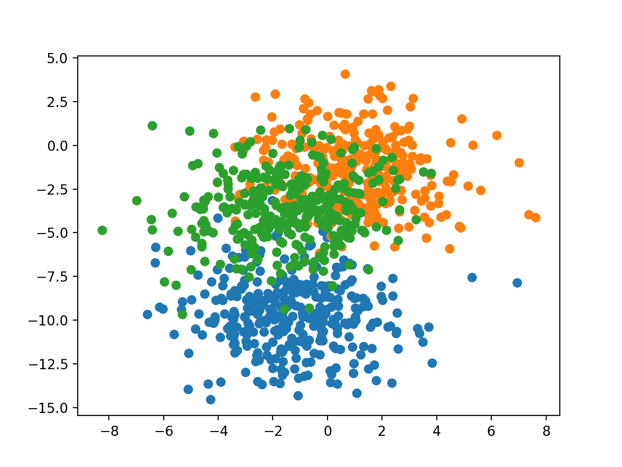
Scatter Plot of Blobs Dataset With Three Classes and Points Colored by Class Value
MLP Fit With Batch Gradient Descent
We can develop a Multilayer Perceptron model (MLP) to address the multi-class classification problem described in the previous section and train it using batch gradient descent.
Firstly, we need to one hot encode the target variable, transforming the integer class values into binary vectors. This will allow the model to predict the probability of each example belonging to each of the three classes, providing more nuance in the predictions and context when training the model.
|
1 2 |
# one hot encode output variable y = to_categorical(y) |
Next, we will split the training dataset of 1,000 examples into a train and test dataset with 500 examples each.
This even split will allow us to evaluate and compare the performance of different configurations of the batch size on the model and its performance.
|
1 2 3 4 |
# split into train and test n_train = 500 trainX, testX = X[:n_train, :], X[n_train:, :] trainy, testy = y[:n_train], y[n_train:] |
We will define an MLP model with an input layer that expects two input variables, for the two variables in the dataset.
The model will have a single hidden layer with 50 nodes and a rectified linear activation function and He random weight initialization. Finally, the output layer has 3 nodes in order to make predictions for the three classes and a softmax activation function.
|
1 2 3 4 |
# define model model = Sequential() model.add(Dense(50, input_dim=2, activation='relu', kernel_initializer='he_uniform')) model.add(Dense(3, activation='softmax')) |
We will optimize the model with stochastic gradient descent and use categorical cross entropy to calculate the error of the model during training.
In this example, we will use “batch gradient descent“, meaning that the batch size will be set to the size of the training dataset. The model will be fit for 200 training epochs and the test dataset will be used as the validation set in order to monitor the performance of the model on a holdout set during training.
The effect will be more time between weight updates and we would expect faster training than other batch sizes, and more stable estimates of the gradient, which should result in a more stable performance of the model during training.
|
1 2 3 4 5 |
# compile model opt = SGD(lr=0.01, momentum=0.9) model.compile(loss='categorical_crossentropy', optimizer=opt, metrics=['accuracy']) # fit model history = model.fit(trainX, trainy, validation_data=(testX, testy), epochs=200, verbose=0, batch_size=len(trainX)) |
Once the model is fit, the performance is evaluated and reported on the train and test datasets.
|
1 2 3 4 |
# evaluate the model _, train_acc = model.evaluate(trainX, trainy, verbose=0) _, test_acc = model.evaluate(testX, testy, verbose=0) print('Train: %.3f, Test: %.3f' % (train_acc, test_acc)) |
A line plot is created showing the train and test set accuracy of the model for each training epoch.
These learning curves provide an indication of three things: how quickly the model learns the problem, how well it has learned the problem, and how noisy the updates were to the model during training.
|
1 2 3 4 5 |
# plot training history pyplot.plot(history.history['accuracy'], label='train') pyplot.plot(history.history['val_accuracy'], label='test') pyplot.legend() pyplot.show() |
Tying these elements together, the complete example is listed below.
|
1 2 3 4 5 6 7 8 9 10 11 12 13 14 15 16 17 18 19 20 21 22 23 24 25 26 27 28 29 30 31 32 33 |
# mlp for the blobs problem with batch gradient descent from sklearn.datasets import make_blobs from keras.layers import Dense from keras.models import Sequential from keras.optimizers import SGD from keras.utils import to_categorical from matplotlib import pyplot # generate 2d classification dataset X, y = make_blobs(n_samples=1000, centers=3, n_features=2, cluster_std=2, random_state=2) # one hot encode output variable y = to_categorical(y) # split into train and test n_train = 500 trainX, testX = X[:n_train, :], X[n_train:, :] trainy, testy = y[:n_train], y[n_train:] # define model model = Sequential() model.add(Dense(50, input_dim=2, activation='relu', kernel_initializer='he_uniform')) model.add(Dense(3, activation='softmax')) # compile model opt = SGD(lr=0.01, momentum=0.9) model.compile(loss='categorical_crossentropy', optimizer=opt, metrics=['accuracy']) # fit model history = model.fit(trainX, trainy, validation_data=(testX, testy), epochs=200, verbose=0, batch_size=len(trainX)) # evaluate the model _, train_acc = model.evaluate(trainX, trainy, verbose=0) _, test_acc = model.evaluate(testX, testy, verbose=0) print('Train: %.3f, Test: %.3f' % (train_acc, test_acc)) # plot training history pyplot.plot(history.history['accuracy'], label='train') pyplot.plot(history.history['val_accuracy'], label='test') pyplot.legend() pyplot.show() |
Running the example first reports the performance of the model on the train and test datasets.
Note: Your results may vary given the stochastic nature of the algorithm or evaluation procedure, or differences in numerical precision. Consider running the example a few times and compare the average outcome.
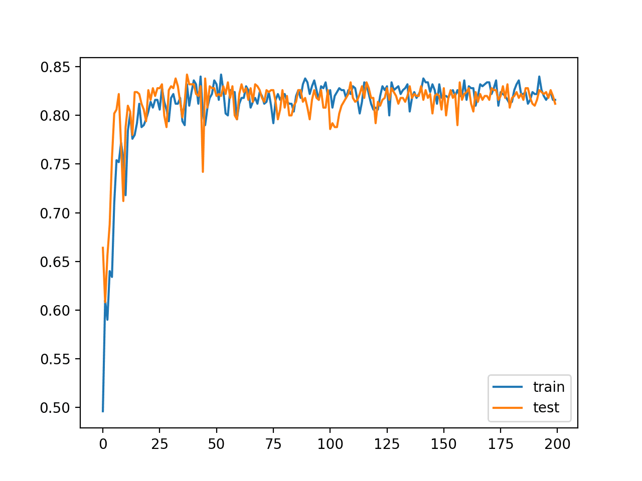
In this case, we can see that performance was similar between the train and test sets with 81% and 83% respectively.
|
1 |
Train: 0.816, Test: 0.830 |
A line plot of model classification accuracy on the train (blue) and test (orange) dataset is created. We can see that the model is relatively slow to learn this problem, converging on a solution after about 100 epochs after which changes in model performance are minor.
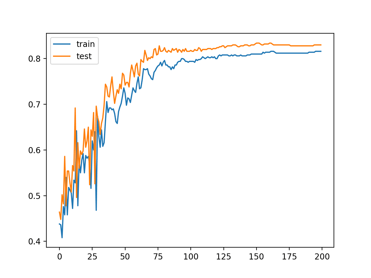
Line Plot of Classification Accuracy on Train and Tests Sets of an MLP Fit With Batch Gradient Descent
MLP Fit With Stochastic Gradient Descent
The example of batch gradient descent from the previous section can be updated to instead use stochastic gradient descent.
This requires changing the batch size from the size of the training dataset to 1.
|
1 2 |
# fit model history = model.fit(trainX, trainy, validation_data=(testX, testy), epochs=200, verbose=0, batch_size=1) |
Stochastic gradient descent requires that the model make a prediction and have the weights updated for each training example. This has the effect of dramatically slowing down the training process as compared to batch gradient descent.
The expectation of this change is that the model learns faster and that changes to the model are noisy, resulting, in turn, in noisy performance over training epochs.
The complete example with this change is listed below.
|
1 2 3 4 5 6 7 8 9 10 11 12 13 14 15 16 17 18 19 20 21 22 23 24 25 26 27 28 29 30 31 32 33 |
# mlp for the blobs problem with stochastic gradient descent from sklearn.datasets import make_blobs from keras.layers import Dense from keras.models import Sequential from keras.optimizers import SGD from keras.utils import to_categorical from matplotlib import pyplot # generate 2d classification dataset X, y = make_blobs(n_samples=1000, centers=3, n_features=2, cluster_std=2, random_state=2) # one hot encode output variable y = to_categorical(y) # split into train and test n_train = 500 trainX, testX = X[:n_train, :], X[n_train:, :] trainy, testy = y[:n_train], y[n_train:] # define model model = Sequential() model.add(Dense(50, input_dim=2, activation='relu', kernel_initializer='he_uniform')) model.add(Dense(3, activation='softmax')) # compile model opt = SGD(lr=0.01, momentum=0.9) model.compile(loss='categorical_crossentropy', optimizer=opt, metrics=['accuracy']) # fit model history = model.fit(trainX, trainy, validation_data=(testX, testy), epochs=200, verbose=0, batch_size=1) # evaluate the model _, train_acc = model.evaluate(trainX, trainy, verbose=0) _, test_acc = model.evaluate(testX, testy, verbose=0) print('Train: %.3f, Test: %.3f' % (train_acc, test_acc)) # plot training history pyplot.plot(history.history['accuracy'], label='train') pyplot.plot(history.history['val_accuracy'], label='test') pyplot.legend() pyplot.show() |
Running the example first reports the performance of the model on the train and test datasets.
Note: Your results may vary given the stochastic nature of the algorithm or evaluation procedure, or differences in numerical precision. Consider running the example a few times and compare the average outcome.
In this case, we can see that performance was similar between the train and test sets, around 60% accuracy, but was dramatically worse (about 20 percentage points) than using batch gradient descent.
At least for this problem and the chosen model and model configuration, stochastic (online) gradient descent is not appropriate.
|
1 |
Train: 0.612, Test: 0.606 |
A line plot of model classification accuracy on the train (blue) and test (orange) dataset is created.
The plot shows the unstable nature of the training process with the chosen configuration. The poor performance and violent changes to the model suggest that the learning rate used to update weights after each training example may be too large and that a smaller learning rate may make the learning process more stable.
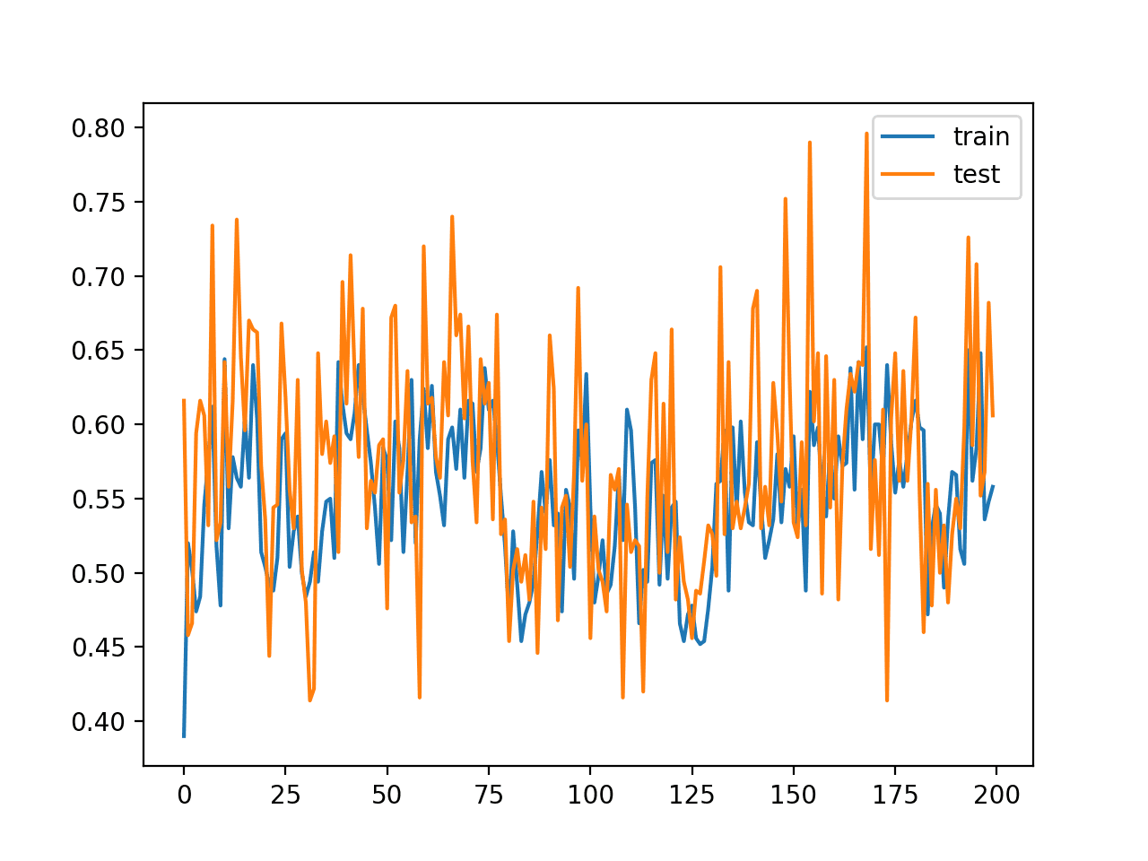
Line Plot of Classification Accuracy on Train and Tests Sets of an MLP Fit With Stochastic Gradient Descent
We can test this by re-running the model fit with stochastic gradient descent and a smaller learning rate. For example, we can drop the learning rate by an order of magnitude form 0.01 to 0.001.
|
1 2 3 |
# compile model opt = SGD(lr=0.001, momentum=0.9) model.compile(loss='categorical_crossentropy', optimizer=opt, metrics=['accuracy']) |
The full code listing with this change is provided below for completeness.
|
1 2 3 4 5 6 7 8 9 10 11 12 13 14 15 16 17 18 19 20 21 22 23 24 25 26 27 28 29 30 31 32 33 |
# mlp for the blobs problem with stochastic gradient descent from sklearn.datasets import make_blobs from keras.layers import Dense from keras.models import Sequential from keras.optimizers import SGD from keras.utils import to_categorical from matplotlib import pyplot # generate 2d classification dataset X, y = make_blobs(n_samples=1000, centers=3, n_features=2, cluster_std=2, random_state=2) # one hot encode output variable y = to_categorical(y) # split into train and test n_train = 500 trainX, testX = X[:n_train, :], X[n_train:, :] trainy, testy = y[:n_train], y[n_train:] # define model model = Sequential() model.add(Dense(50, input_dim=2, activation='relu', kernel_initializer='he_uniform')) model.add(Dense(3, activation='softmax')) # compile model opt = SGD(lr=0.001, momentum=0.9) model.compile(loss='categorical_crossentropy', optimizer=opt, metrics=['accuracy']) # fit model history = model.fit(trainX, trainy, validation_data=(testX, testy), epochs=200, verbose=0, batch_size=1) # evaluate the model _, train_acc = model.evaluate(trainX, trainy, verbose=0) _, test_acc = model.evaluate(testX, testy, verbose=0) print('Train: %.3f, Test: %.3f' % (train_acc, test_acc)) # plot training history pyplot.plot(history.history['accuracy'], label='train') pyplot.plot(history.history['val_accuracy'], label='test') pyplot.legend() pyplot.show() |
Running this example tells a very different story.
Note: Your results may vary given the stochastic nature of the algorithm or evaluation procedure, or differences in numerical precision. Consider running the example a few times and compare the average outcome.
The reported performance is greatly improved, achieving classification accuracy on the train and test sets on par with fit using batch gradient descent.
|
1 |
Train: 0.816, Test: 0.824 |
The line plot shows the expected behavior. Namely, that the model rapidly learns the problem as compared to batch gradient descent, leaping up to about 80% accuracy in about 25 epochs rather than the 100 epochs seen when using batch gradient descent. We could have stopped training at epoch 50 instead of epoch 200 due to the faster training.
This is not surprising. With batch gradient descent, 100 epochs involved 100 estimates of error and 100 weight updates. In stochastic gradient descent, 25 epochs involved (500 * 25) or 12,500 weight updates, providing more than 10-times more feedback, albeit more noisy feedback, about how to improve the model.
The line plot also shows that train and test performance remain comparable during training, as compared to the dynamics with batch gradient descent where the performance on the test set was slightly better and remained so throughout training.
Unlike batch gradient descent, we can see that the noisy updates result in noisy performance throughout the duration of training. This variance in the model means that it may be challenging to choose which model to use as the final model, as opposed to batch gradient descent where performance is stabilized because the model has converged.
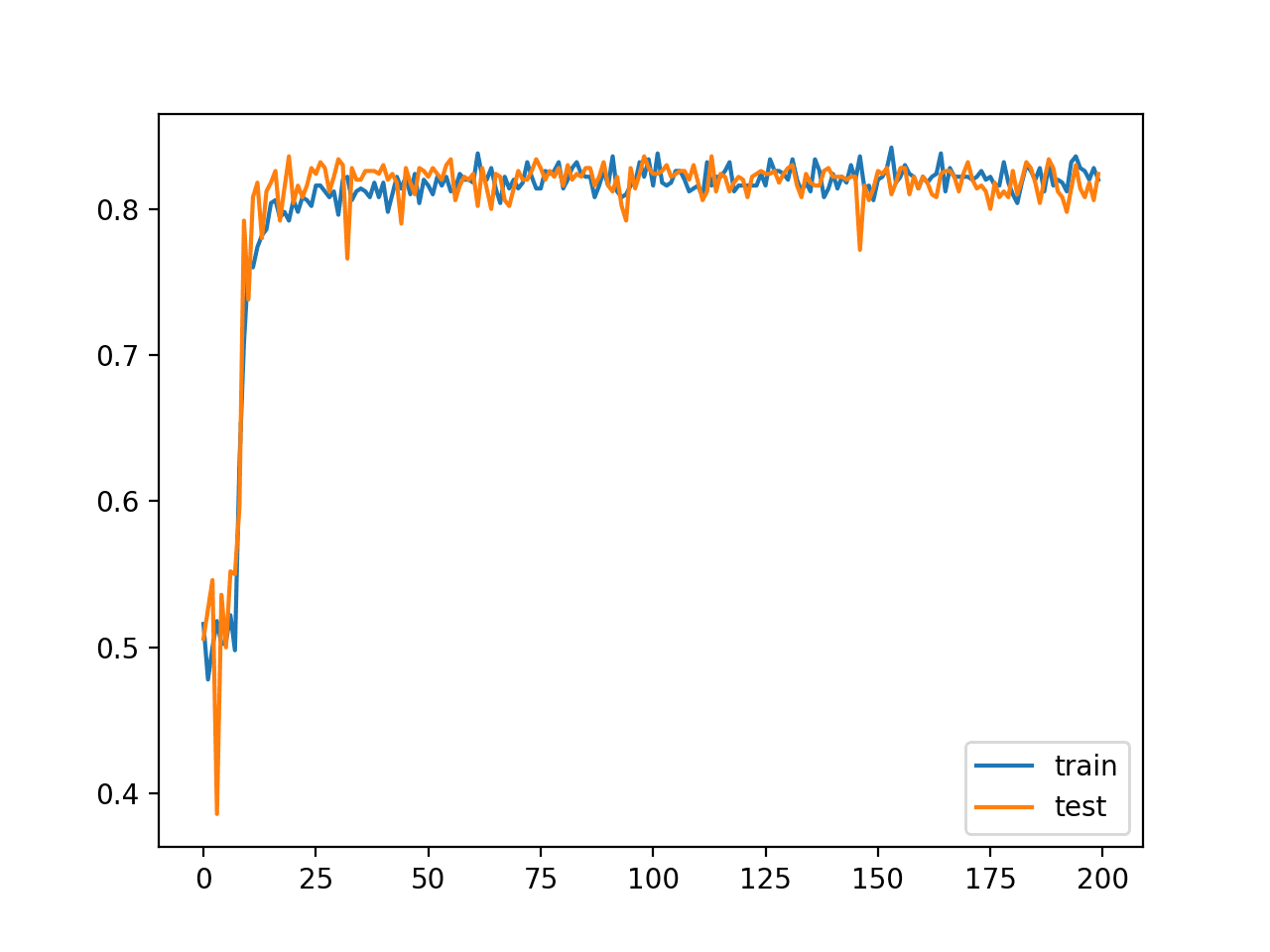
Line Plot of Classification Accuracy on Train and Tests Sets of an MLP Fit With Stochastic Gradient Descent and Smaller Learning Rate
This example highlights the important relationship between batch size and the learning rate. Namely, more noisy updates to the model require a smaller learning rate, whereas less noisy more accurate estimates of the error gradient may be applied to the model more liberally. We can summarize this as follows:
- Batch Gradient Descent: Use a relatively larger learning rate and more training epochs.
- Stochastic Gradient Descent: Use a relatively smaller learning rate and fewer training epochs.
Mini-batch gradient descent provides an alternative approach.
MLP Fit With Minibatch Gradient Descent
An alternative to using stochastic gradient descent and tuning the learning rate is to hold the learning rate constant and to change the batch size.
In effect, it means that we specify the rate of learning or amount of change to apply to the weights each time we estimate the error gradient, but to vary the accuracy of the gradient based on the number of samples used to estimate it.
Holding the learning rate at 0.01 as we did with batch gradient descent, we can set the batch size to 32, a widely adopted default batch size.
|
1 2 |
# fit model history = model.fit(trainX, trainy, validation_data=(testX, testy), epochs=200, verbose=0, batch_size=32) |
We would expect to get some of the benefits of stochastic gradient descent with a larger learning rate.
The complete example with this modification is listed below.
|
1 2 3 4 5 6 7 8 9 10 11 12 13 14 15 16 17 18 19 20 21 22 23 24 25 26 27 28 29 30 31 32 33 |
# mlp for the blobs problem with minibatch gradient descent from sklearn.datasets import make_blobs from keras.layers import Dense from keras.models import Sequential from keras.optimizers import SGD from keras.utils import to_categorical from matplotlib import pyplot # generate 2d classification dataset X, y = make_blobs(n_samples=1000, centers=3, n_features=2, cluster_std=2, random_state=2) # one hot encode output variable y = to_categorical(y) # split into train and test n_train = 500 trainX, testX = X[:n_train, :], X[n_train:, :] trainy, testy = y[:n_train], y[n_train:] # define model model = Sequential() model.add(Dense(50, input_dim=2, activation='relu', kernel_initializer='he_uniform')) model.add(Dense(3, activation='softmax')) # compile model opt = SGD(lr=0.01, momentum=0.9) model.compile(loss='categorical_crossentropy', optimizer=opt, metrics=['accuracy']) # fit model history = model.fit(trainX, trainy, validation_data=(testX, testy), epochs=200, verbose=0, batch_size=32) # evaluate the model _, train_acc = model.evaluate(trainX, trainy, verbose=0) _, test_acc = model.evaluate(testX, testy, verbose=0) print('Train: %.3f, Test: %.3f' % (train_acc, test_acc)) # plot training history pyplot.plot(history.history['accuracy'], label='train') pyplot.plot(history.history['val_accuracy'], label='test') pyplot.legend() pyplot.show() |
Note: Your results may vary given the stochastic nature of the algorithm or evaluation procedure, or differences in numerical precision. Consider running the example a few times and compare the average outcome.
Running the example reports similar performance on both train and test sets, comparable with batch gradient descent and stochastic gradient descent after we reduced the learning rate.
|
1 |
Train: 0.832, Test: 0.812 |
The line plot shows the dynamics of both stochastic and batch gradient descent. Specifically, the model learns fast and has noisy updates but also stabilizes more towards the end of the run, more so than stochastic gradient descent.
Holding learning rate constant and varying the batch size allows you to dial in the best of both approaches.
Line Plot of Classification Accuracy on Train and Tests Sets of an MLP Fit With Minibatch Gradient Descent
Effect of Batch Size on Model Behavior
We can refit the model with different batch sizes and review the impact the change in batch size has on the speed of learning, stability during learning, and on the final result.
First, we can clean up the code and create a function to prepare the dataset.
|
1 2 3 4 5 6 7 8 9 10 11 |
# prepare train and test dataset def prepare_data(): # generate 2d classification dataset X, y = make_blobs(n_samples=1000, centers=3, n_features=2, cluster_std=2, random_state=2) # one hot encode output variable y = to_categorical(y) # split into train and test n_train = 500 trainX, testX = X[:n_train, :], X[n_train:, :] trainy, testy = y[:n_train], y[n_train:] return trainX, trainy, testX, testy |
Next, we can create a function to fit a model on the problem with a given batch size and plot the learning curves of classification accuracy on the train and test datasets.
|
1 2 3 4 5 6 7 8 9 10 11 12 13 14 15 |
# fit a model and plot learning curve def fit_model(trainX, trainy, testX, testy, n_batch): # define model model = Sequential() model.add(Dense(50, input_dim=2, activation='relu', kernel_initializer='he_uniform')) model.add(Dense(3, activation='softmax')) # compile model opt = SGD(lr=0.01, momentum=0.9) model.compile(loss='categorical_crossentropy', optimizer=opt, metrics=['accuracy']) # fit model history = model.fit(trainX, trainy, validation_data=(testX, testy), epochs=200, verbose=0, batch_size=n_batch) # plot learning curves pyplot.plot(history.history['accuracy'], label='train') pyplot.plot(history.history['val_accuracy'], label='test') pyplot.title('batch='+str(n_batch), pad=-40) |
Finally, we can evaluate the model behavior with a suite of different batch sizes while holding everything else about the model constant, including the learning rate.
|
1 2 3 4 5 6 7 8 9 10 11 12 |
# prepare dataset trainX, trainy, testX, testy = prepare_data() # create learning curves for different batch sizes batch_sizes = [4, 8, 16, 32, 64, 128, 256, 450] for i in range(len(batch_sizes)): # determine the plot number plot_no = 420 + (i+1) pyplot.subplot(plot_no) # fit model and plot learning curves for a batch size fit_model(trainX, trainy, testX, testy, batch_sizes[i]) # show learning curves pyplot.show() |
The result will be a figure with eight plots of model behavior with eight different batch sizes.
Tying this together, the complete example is listed below.
|
1 2 3 4 5 6 7 8 9 10 11 12 13 14 15 16 17 18 19 20 21 22 23 24 25 26 27 28 29 30 31 32 33 34 35 36 37 38 39 40 41 42 43 44 45 46 47 48 |
# mlp for the blobs problem with minibatch gradient descent with varied batch size from sklearn.datasets import make_blobs from keras.layers import Dense from keras.models import Sequential from keras.optimizers import SGD from keras.utils import to_categorical from matplotlib import pyplot # prepare train and test dataset def prepare_data(): # generate 2d classification dataset X, y = make_blobs(n_samples=1000, centers=3, n_features=2, cluster_std=2, random_state=2) # one hot encode output variable y = to_categorical(y) # split into train and test n_train = 500 trainX, testX = X[:n_train, :], X[n_train:, :] trainy, testy = y[:n_train], y[n_train:] return trainX, trainy, testX, testy # fit a model and plot learning curve def fit_model(trainX, trainy, testX, testy, n_batch): # define model model = Sequential() model.add(Dense(50, input_dim=2, activation='relu', kernel_initializer='he_uniform')) model.add(Dense(3, activation='softmax')) # compile model opt = SGD(lr=0.01, momentum=0.9) model.compile(loss='categorical_crossentropy', optimizer=opt, metrics=['accuracy']) # fit model history = model.fit(trainX, trainy, validation_data=(testX, testy), epochs=200, verbose=0, batch_size=n_batch) # plot learning curves pyplot.plot(history.history['accuracy'], label='train') pyplot.plot(history.history['val_accuracy'], label='test') pyplot.title('batch='+str(n_batch), pad=-40) # prepare dataset trainX, trainy, testX, testy = prepare_data() # create learning curves for different batch sizes batch_sizes = [4, 8, 16, 32, 64, 128, 256, 450] for i in range(len(batch_sizes)): # determine the plot number plot_no = 420 + (i+1) pyplot.subplot(plot_no) # fit model and plot learning curves for a batch size fit_model(trainX, trainy, testX, testy, batch_sizes[i]) # show learning curves pyplot.show() |
Running the example creates a figure with eight line plots showing the classification accuracy on the train and test sets of models with different batch sizes when using mini-batch gradient descent.
Note: Your results may vary given the stochastic nature of the algorithm or evaluation procedure, or differences in numerical precision. Consider running the example a few times and compare the average outcome.
The plots show that small batch results generally in rapid learning but a volatile learning process with higher variance in the classification accuracy. Larger batch sizes slow down the learning process but the final stages result in a convergence to a more stable model exemplified by lower variance in classification accuracy.
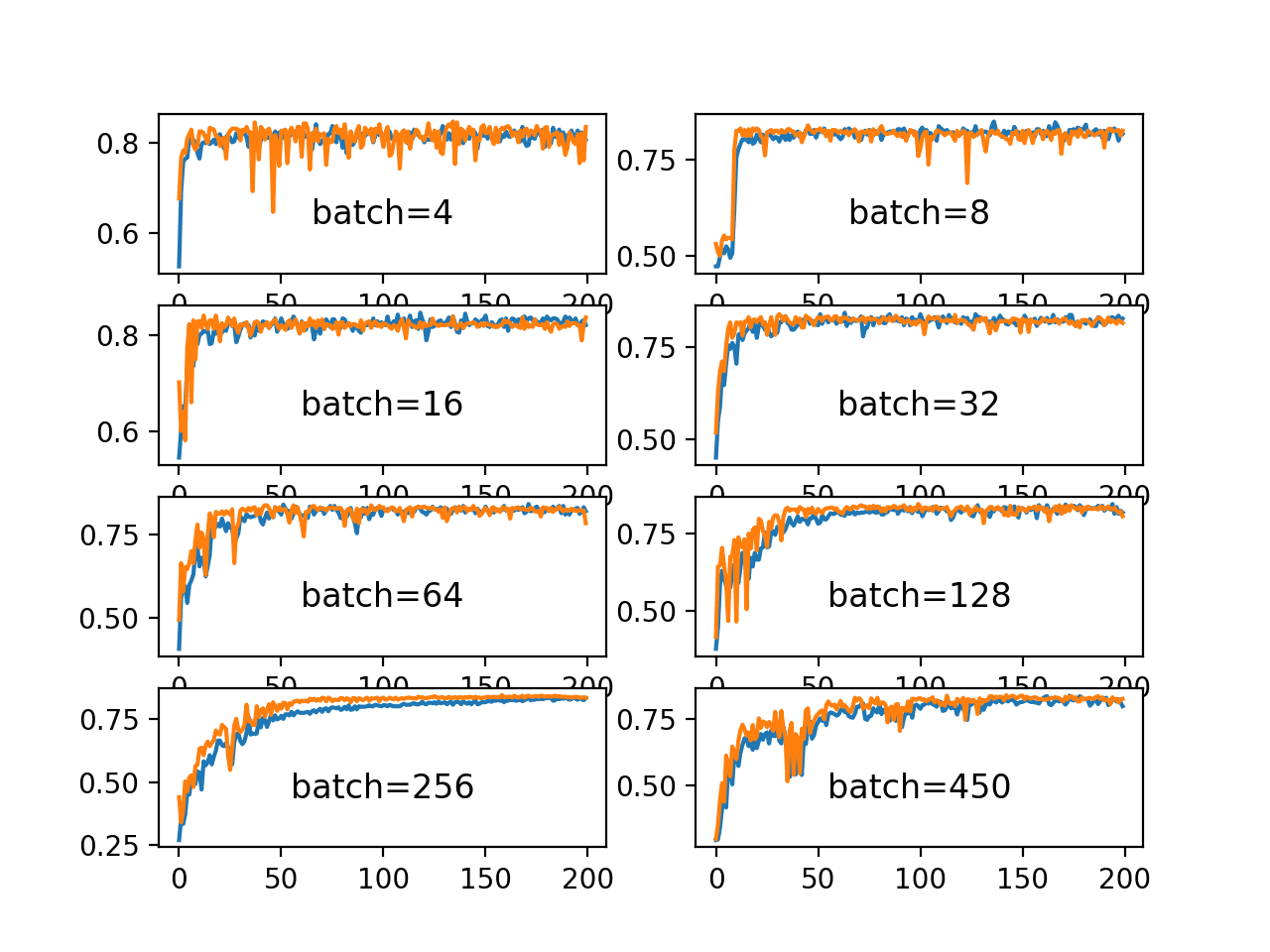
Line Plots of Classification Accuracy on Train and Test Datasets With Different Batch Sizes
Further Reading
This section provides more resources on the topic if you are looking to go deeper.
Posts
Papers
- Revisiting Small Batch Training for Deep Neural Networks, 2018.
- Practical recommendations for gradient-based training of deep architectures, 2012.
Books
- 8.1.3 Batch and Minibatch Algorithms, Deep Learning, 2016.
Articles
Summary
In this tutorial, you discovered three different flavors of gradient descent and how to explore and diagnose the effect of batch size on the learning process.
Specifically, you learned:
- Batch size controls the accuracy of the estimate of the error gradient when training neural networks.
- Batch, Stochastic, and Minibatch gradient descent are the three main flavors of the learning algorithm.
- There is a tension between batch size and the speed and stability of the learning process.
Do you have any questions?
Ask your questions in the comments below and I will do my best to answer.
Develop Better Deep Learning Models Today!

Train Faster, Reduce Overftting, and Ensembles
...with just a few lines of python code
Discover how in my new Ebook:
Better Deep Learning
It provides self-study tutorials on topics like:
weight decay, batch normalization, dropout, model stacking and much more...
Bring better deep learning to your projects!
Skip the Academics. Just Results.


I always thank you for information.
I have learned a lot from your blog.
I have one quesiton regarding Stateless LSTM network with batch_size 1 and fixed sliding window.
This LSTM model outperforms other classical method such as polynomial and MLP model.
In this setting, this LSTM model is almost the same as normal MLP Becasue cell state is reset after each batch.
I do not take any advantage of LSTM model. Of course, there are more parameters in each LSTM layer. But this is not enough to explain the result.
Can you give some intuitive advice?
Is it worth using LSTM in this case?
Interesting. I would expect that an MLP would be able to outperform such an LSTM.
Perhaps try this approach:
https://machinelearningmastery.com/how-to-develop-a-skilful-time-series-forecasting-model/
Thank you so much this is one of your best articles ever. I had taken Andrew ngs full 5 courses class and still did not grasp this so great job. Only took 15 minutes to grasp 🙂
Thanks Todd!
same here
Very nice article. I have a question about the last figure. I notice the plots have different scales on the Y axis. Does it imply that batch-4 and batch-16 have converged with better overall accuracy?
Great comment! Ideally the plots would all have the same y-axis.
In this case, I don’t expect the y axis to differ, only the choice of labels printed.
very nice article. i learned a lot from this !!!!!
Thanks, I’m glad it helped.
Hi Jason,
thanks for your article,
I have a question,
does number of category (y) has any relation with batch_size ?
suppose we have 150 category to classify and if we initialize batch_size=32,
In one batch, our process won’t be able to train all type of class, hence learning will be very slow ?
Please correct me if i m wrong
Great question!
We want the batch to contain a diverse set of examples. If you have 150 categories, perhaps a larger batch size would be more repetitive of the dataset.
Test it and see.
Hi Jason,
As you suggested to train with larger batch size if we have more categories let say 150 in above case. But most of time I face GPU ram challenge so how can I approach this problem any other way ?
Perhaps some of the suggestions here:
https://machinelearningmastery.com/improve-deep-learning-performance/
Dear Dr.Brownlee,
thank you so much for your useful information.
i have learned a lot of things from your blog.
kind regard,
Abolfazl Nejatian
Thanks, I’m glad the tutorials helped.
Hi, thank you for this article which is very clear, with very nice examples.
I have a question:
Regarding the last figure with the eight graphics, would it be insteresting to imagine a dynamic batch size?
I mean we could start the learning process with a very small batch size (say 4) to get a fast but coarse convergence and then we could increase the batch size (say 256) to get the stability?
May be it will be faster than Batch Gradient Descent and steadier than stochastic gradient descent, isn’t it?
Regards
Romain Schuster, PhD
You’re welcome!
You could, perhaps try it!
We typically fix the batch size for efficiency reasons – so we can prepare the structures (in tensorflow) fast computation.
Hi Schuster,
There is an article that supports this hypothesis which you may be interested in: https://openreview.net/pdf?id=B1Yy1BxCZ
Cheers,
AG
Thanks for sharing!
WHat does that 420 do in the plot_no?
Sorry, I don’t understand your question.
Can you please elaborate?
HI,
Based on your post and some more related posted I came across this repository and have doubts on what is the use of normalizing the weight initialization. can you help-
https://github.com/PranaySPatil/ComputerVision-CSCI5561/tree/master/HW4
If you have questions about the repository, perhaps contact the author directly.
Keeping the learning rate constant, what would be the effect of increasing/decreasing
batch size on NN training?
Probably slower or faster learning – but to a point given the quality of the gradient estimates.
Hi, I have a doubt. I am having sparse matrices and I wanted to train a sparse mlp. If given sparse=True in keras input layer, which is followed by dense layer, it throws error. But the same code works in colab but in kaggle kernel I face this issue. Any idea?
Not offhand sorry, you will need to debug your code to discover the answer, or try posting the code and error to stackoverflow.
Thanks! I will surely do that. Your posts are of great help. Thank You so much.
You’re welcome.
Hi Jason,
Thank you so much for this incredible source of information.
I have a question, probably a basic one, so I apologize in advance.
On the model accuracy plot (first figure), the test set has better accuracy than the training set. What would be the explanation for this? I was under the impression that the test accuracy is always expected to be slightly worse, given that the test data is new to the model.
Best,
Stani
You’re welcome!
This can help you interpret learning curves:
https://machinelearningmastery.com/learning-curves-for-diagnosing-machine-learning-model-performance/
Hi Jason thanks for this tutorial. I have a quetion,
what about model.fit_generator() how can we change the batch_size on it?
“steps_per_epoch” controls the number of batches in one epoch of your training dataset.
Thank you Jason for such a useful page. Umm I am newbie to ML world , and my question may be silly ,but i am really confused about it. you mentioned that using small batch size, the learning would be quick and vice versa. However, I implemented the code and noticed that using small number for mini batch size takes longer time than using large number. Could you pls explain to me why is that happens? did i misunderstand the idea?
your time is totaly appreciated
You’re welcome.
Yes, smaller batch size means more calculation and more updates to the model weights, which is slower.
Larger batch size does less work and is faster to execute.
Hi Jason.
Thanks, for you insightful topic.
I have question :
how about if it’s trapped in local minimum(let’s say mainly because that first random weight initialize) . When we re-run again sometimes it’s go to direction of global minimum. But sometimes is not… sometimes it’s going to direction of local minimum. As NN is using gradient as direction to go.(as trap in local minimun, gradient just back and forth)
I ever encounter this situation, even playing batch number, doesn’t help, as somehow
the “beginning weight during random initialize” is seems really determine the “first direction”
I heard about simulated annealing that can try “jump” to other place from local minimum, but I am not sure is this method exist in Keras.
any hint
Thanks
Mike
One approach is to fit many model and average their predictions.
Another is to fit many models and choose the one that performs the best on a hold out validation set.
Hi Jason, another great post.
Now, for the first time in my life, I am trying Keras’ tuner’s BayesianOptimization() function for hyperparameter tuning.
In this setting, how can I incorporate optimization of batch size?
Do you have any good example?
Hi Michio…Thank you for your feedback! The following resource provides a great introduction to an amazing bayesian optimization tuner with examples.
https://github.com/bayesian-optimization/BayesianOptimization