A sample of data will form a distribution, and by far the most well-known distribution is the Gaussian distribution, often called the Normal distribution.
The distribution provides a parameterized mathematical function that can be used to calculate the probability for any individual observation from the sample space. This distribution describes the grouping or the density of the observations, called the probability density function. We can also calculate the likelihood of an observation having a value equal to or lesser than a given value. A summary of these relationships between observations is called a cumulative density function.
In this tutorial, you will discover the Gaussian and related distribution functions and how to calculate probability and cumulative density functions for each.
After completing this tutorial, you will know:
A gentle introduction to standard distributions to summarize the relationship of observations.
How to calculate and plot probability and density functions for the Gaussian distribution.
The Student t and Chi-squared distributions related to the Gaussian distribution.
Kick-start your project with my new book Statistics for Machine Learning, including step-by-step tutorials and the Python source code files for all examples.
Let’s get started.
A Gentle Introduction to Statistical Data Distributions Photo by Ed Dunens, some rights reserved.
Tutorial Overview
This tutorial is divided into 4 parts; they are:
Distributions
Gaussian Distribution
Student’s t-Distribution
Chi-Squared Distribution
Need help with Statistics for Machine Learning?
Take my free 7-day email crash course now (with sample code).
Click to sign-up and also get a free PDF Ebook version of the course.
Distributions
From a practical perspective, we can think of a distribution as a function that describes the relationship between observations in a sample space.
For example, we may be interested in the age of humans, with individual ages representing observations in the domain, and ages 0 to 125 the extent of the sample space. The distribution is a mathematical function that describes the relationship of observations of different heights.
A distribution is simply a collection of data, or scores, on a variable. Usually, these scores are arranged in order from smallest to largest and then they can be presented graphically.
Many data conform to well-known and well-understood mathematical functions, such as the Gaussian distribution. A function can fit the data with a modification of the parameters of the function, such as the mean and standard deviation in the case of the Gaussian.
Once a distribution function is known, it can be used as a shorthand for describing and calculating related quantities, such as likelihoods of observations, and plotting the relationship between observations in the domain.
Density Functions
Distributions are often described in terms of their density or density functions.
Density functions are functions that describe how the proportion of data or likelihood of the proportion of observations change over the range of the distribution.
Two types of density functions are probability density functions and cumulative density functions.
Probability Density function: calculates the probability of observing a given value.
Cumulative Density function: calculates the probability of an observation equal or less than a value.
A probability density function, or PDF, can be used to calculate the likelihood of a given observation in a distribution. It can also be used to summarize the likelihood of observations across the distribution’s sample space. Plots of the PDF show the familiar shape of a distribution, such as the bell-curve for the Gaussian distribution.
Distributions are often defined in terms of their probability density functions with their associated parameters.
A cumulative density function, or CDF, is a different way of thinking about the likelihood of observed values. Rather than calculating the likelihood of a given observation as with the PDF, the CDF calculates the cumulative likelihood for the observation and all prior observations in the sample space. It allows you to quickly understand and comment on how much of the distribution lies before and after a given value. A CDF is often plotted as a curve from 0 to 1 for the distribution.
Both PDFs and CDFs are continuous functions. The equivalent of a PDF for a discrete distribution is called a probability mass function, or PMF.
Next, let’s look at the Gaussian distribution and two other distributions related to the Gaussian that you will encounter when using statistical methods. We will look at each in turn in terms of their parameters, probability, and cumulative density functions.
Gaussian Distribution
The Gaussian distribution, named for Carl Friedrich Gauss, is the focus of much of the field of statistics.
Data from many fields of study surprisingly can be described using a Gaussian distribution, so much so that the distribution is often called the “normal” distribution because it is so common.
A Gaussian distribution can be described using two parameters:
mean: Denoted with the Greek lowercase letter mu, is the expected value of the distribution.
variance: Denoted with the Greek lowercase letter sigma raised to the second power (because the units of the variable are squared), describes the spread of observation from the mean.
It is common to use a normalized calculation of the variance called the standard deviation
standard deviation: Denoted with the Greek lowercase letter sigma, describes the normalized spread of observations from the mean.
We can work with the Gaussian distribution via the norm SciPy module. The norm.pdf() function can be used to create a Gaussian probability density function with a given sample space, mean, and standard deviation.
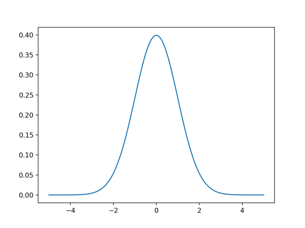
The example below creates a Gaussian PDF with a sample space from -5 to 5, a mean of 0, and a standard deviation of 1. A Gaussian with these values for the mean and standard deviation is called the Standard Gaussian.
1
2
3
4
5
6
7
8
9
10
11
12
13
# plot the gaussian pdf
from numpy import arange
from matplotlib import pyplot
from scipy.stats import norm
# define the distribution parameters
sample_space=arange(-5,5,0.001)
mean=0.0
stdev=1.0
# calculate the pdf
pdf=norm.pdf(sample_space,mean,stdev)
# plot
pyplot.plot(sample_space,pdf)
pyplot.show()
Running the example creates a line plot showing the sample space in the x-axis and the likelihood of each value of the y-axis. The line plot shows the familiar bell-shape for the Gaussian distribution.
The top of the bell shows the most likely value from the distribution, called the expected value or the mean, which in this case is zero, as we specified in creating the distribution.
Line Plot of the Gaussian Probability Density Function
The norm.cdf() function can be used to create a Gaussian cumulative density function.
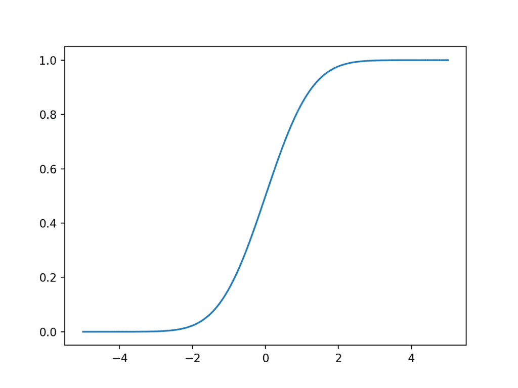
The example below creates a Gaussian CDF for the same sample space.
1
2
3
4
5
6
7
8
9
10
11
# plot the gaussian cdf
from numpy import arange
from matplotlib import pyplot
from scipy.stats import norm
# define the distribution parameters
sample_space=arange(-5,5,0.001)
# calculate the cdf
cdf=norm.cdf(sample_space)
# plot
pyplot.plot(sample_space,cdf)
pyplot.show()
Running the example creates a plot showing an S-shape with the sample space on the x-axis and the cumulative probability of the y-axis.
We can see that a value of 2 covers close to 100% of the observations, with only a very thin tail of the distribution beyond that point.
We can also see that the mean value of zero shows 50% of the observations before and after that point.
Line Plot of the Gaussian Cumulative Density Function
Student’s t-Distribution
The Student’s t-distribution, or just t-distribution for short, is named for the pseudonym “Student” by William Sealy Gosset.
It is a distribution that arises when attempting to estimate the mean of a normal distribution with different sized samples. As such, it is a helpful shortcut when describing uncertainty or error related to estimating population statistics for data drawn from Gaussian distributions when the size of the sample must be taken into account.
Although you may not use the Student’s t-distribution directly, you may estimate values from the distribution required as parameters in other statistical methods, such as statistical significance tests.
The distribution can be described using a single parameter:
number of degrees of freedom: denoted with the lowercase Greek letter nu (v), denotes the number degrees of freedom.
Key to the use of the t-distribution is knowing the desired number of degrees of freedom.
The number of degrees of freedom describes the number of pieces of information used to describe a population quantity. For example, the mean has n degrees of freedom as all n observations in the sample are used to calculate the estimate of the population mean. A statistical quantity that makes use of another statistical quantity in its calculation must subtract 1 from the degrees of freedom, such as the use of the mean in the calculation of the sample variance.
Observations in a Student’s t-distribution are calculated from observations in a normal distribution in order to describe the interval for the populations mean in the normal distribution. Observations are calculated as:
1
data = (x - mean(x)) / S / sqrt(n)
Where x is the observations from the Gaussian distribution, mean is the average observation of x, S is the standard deviation and n is the total number of observations. The resulting observations form the t-observation with (n – 1) degrees of freedom.
In practice, if you require a value from a t-distribution in the calculation of a statistic, then the number of degrees of freedom will likely be n – 1, where n is the size of your sample drawn from a Gaussian distribution.
Which specific distribution you use for a given problem depends on the size of your sample.
SciPy provides tools for working with the t-distribution in the stats.t module. The t.pdf() function can be used to create a Student t-distribution with the specified degrees of freedom.
The example below creates a t-distribution using the sample space from -5 to 5 and (10,000 – 1) degrees of freedom.
1
2
3
4
5
6
7
8
9
10
11
12
# plot the t-distribution pdf
from numpy import arange
from matplotlib import pyplot
from scipy.stats importt
# define the distribution parameters
sample_space=arange(-5,5,0.001)
dof=len(sample_space)-1
# calculate the pdf
pdf=t.pdf(sample_space,dof)
# plot
pyplot.plot(sample_space,pdf)
pyplot.show()
Running the example creates and plots the t-distribution PDF.
We can see the familiar bell-shape to the distribution much like the normal. A key difference is the fatter tails in the distribution, highlighting the increased likelihood of observations in the tails compared to that of the Gaussian.
Line Plot of the Student’s t-Distribution Probability Density Function
The t.cdf() function can be used to create the cumulative density function for the t-distribution. The example below creates the CDF over the same range as above.
1
2
3
4
5
6
7
8
9
10
11
12
# plot the t-distribution cdf
from numpy import arange
from matplotlib import pyplot
from scipy.stats importt
# define the distribution parameters
sample_space=arange(-5,5,0.001)
dof=len(sample_space)-1
# calculate the cdf
cdf=t.cdf(sample_space,dof)
# plot
pyplot.plot(sample_space,cdf)
pyplot.show()
Running the example, we see the familiar S-shaped curve as we see with the Gaussian distribution, although with slightly softer transitions from zero-probability to one-probability for the fatter tails.
Line Plot of the Student’s t-distribution Cumulative Density Function
Chi-Squared Distribution
The chi-squared distribution is denoted as the lowecase Greek letter chi (X) raised to the second power (X^2).
Like the Student’s t-distribution, the chi-squared distribution is also used in statistical methods on data drawn from a Gaussian distribution to quantify the uncertainty. For example, the chi-squared distribution is used in the chi-squared statistical tests for independence. In fact, the chi-squared distribution is used in the derivation of the Student’s t-distribution.
The chi-squared distribution has one parameter:
degrees of freedom, denoted k.
An observation in a chi-squared distribution is calculated as the sum of k squared observations drawn from a Gaussian distribution.
1
chi = sum x[i]^2 for i=1 to k.
Where chi is an observation that has a chi-squared distribution, x are observation drawn from a Gaussian distribution, and k is the number of x observations which is also the number of degrees of freedom for the chi-squared distribution.
Again, as with the Student’s t-distribution, data does not fit a chi-squared distribution; instead, observations are drawn from this distribution in the calculation of statistical methods for a sample of Gaussian data.
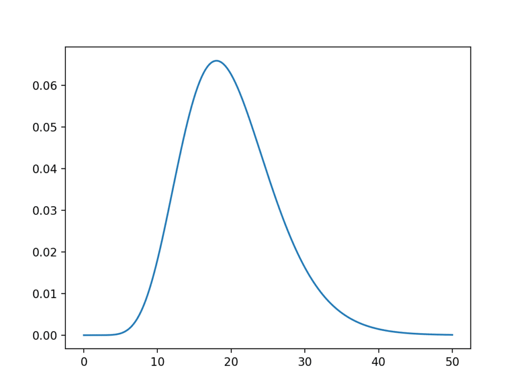
SciPy provides the stats.chi2 module for calculating statistics for the chi-squared distribution. The chi2.pdf() function can be used to calculate the chi-squared distribution for a sample space between 0 and 50 with 20 degrees of freedom. Recall that the sum squared values must be positive, hence the need for a positive sample space.
1
2
3
4
5
6
7
8
9
10
11
12
# plot the chi-squared pdf
from numpy import arange
from matplotlib import pyplot
from scipy.stats import chi2
# define the distribution parameters
sample_space=arange(0,50,0.01)
dof=20
# calculate the pdf
pdf=chi2.pdf(sample_space,dof)
# plot
pyplot.plot(sample_space,pdf)
pyplot.show()
Running the example calculates the chi-squared PDF and presents it as a line plot.
With 20 degrees of freedom, we can see that the expected value of the distribution is just short of the value 20 on the sample space. This is intuitive if we think most of the density in the Gaussian distribution lies between -1 and 1 and then the sum of the squared random observations from the standard Gaussian would sum to just under the number of degrees of freedom, in this case 20.
Although the distribution has a bell-like shape, the distribution is not symmetric.
Line Plot of the Chi-Squared Probability Density Function
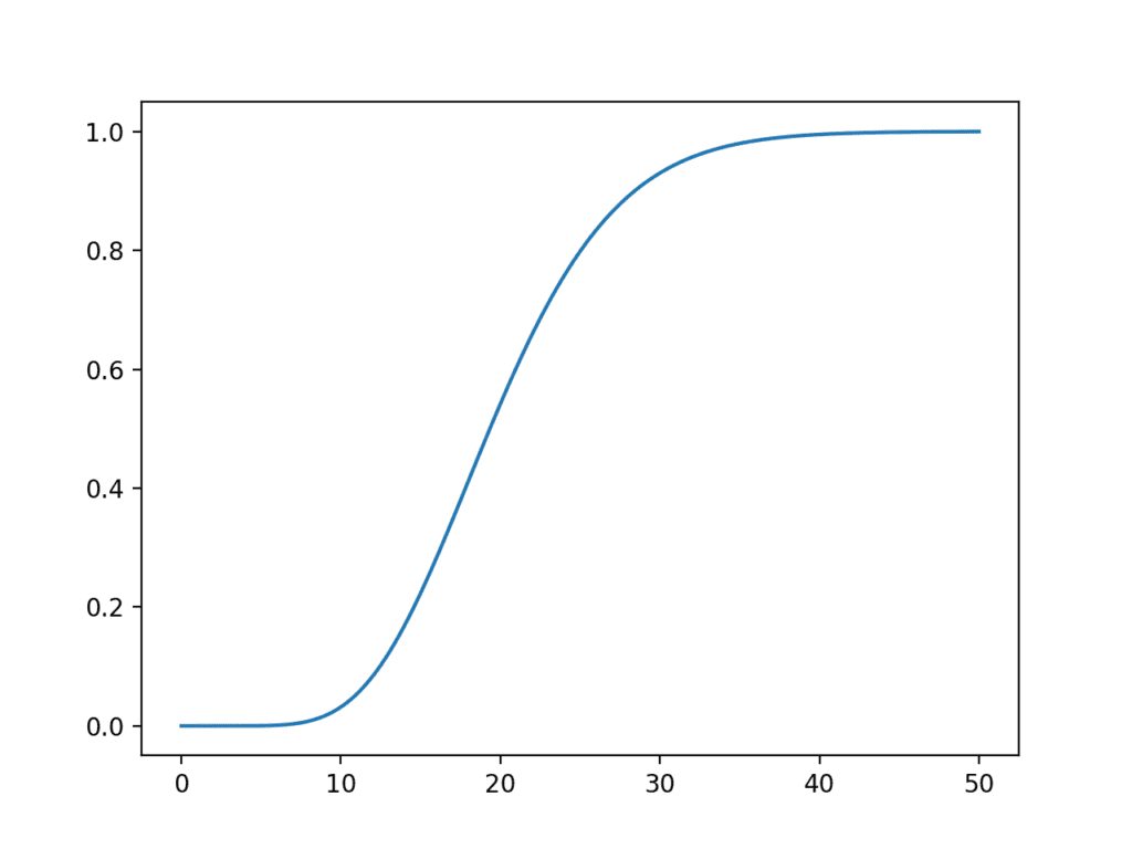
The chi2.cdf() function can be used to calculate the cumulative density function over the same sample space.
1
2
3
4
5
6
7
8
9
10
11
12
# plot the chi-squared cdf
from numpy import arange
from matplotlib import pyplot
from scipy.stats import chi2
# define the distribution parameters
sample_space=arange(0,50,0.01)
dof=20
# calculate the cdf
cdf=chi2.cdf(sample_space,dof)
# plot
pyplot.plot(sample_space,cdf)
pyplot.show()
Running the example creates a plot of the cumulative density function for the chi-squared distribution.
The distribution helps to see the likelihood for the chi-squared value around 20 with the fat tail to the right of the distribution that would continue on long after the end of the plot.
Line Plot of the Chi-squared distribution Cumulative Density Function
Extensions
This section lists some ideas for extending the tutorial that you may wish to explore.
Recreate the PDF and CDF plots for one distribution with a new sample space.
Calculate and plot the PDF and CDF for the Cauchy and Laplace distributions.
Look up and implement the equations for the PDF and CDF for one distribution from scratch.
If you explore any of these extensions, I’d love to know.
Further Reading
This section provides more resources on the topic if you are looking to go deeper.
In this tutorial, you discovered the Gaussian and related distribution functions and how to calculate probability and cumulative density functions for each.
Specifically, you learned:
A gentle introduction to standard distributions to summarize the relationship of observations.
How to calculate and plot probability and density functions for the Gaussian distribution.
The Student t and Chi-squared distributions related to the Gaussian distribution.
Do you have any questions?
Ask your questions in the comments below and I will do my best to answer.
Dear Dr Jason,
This question is about chi-squared distribution.
(1) In the t-test, the dof= len(data)-1. What is the basis of the dof for the chi-square distribution?
(2) The sum(observation**2) follows a chi-squared distribution. What is the point of squaring all observations and summing then when you can make an inference on the unsquared observation using the gaussian or t-dist?
Dear Dr Jason,
I have read the article. The chi-squared test is used for a number of hypothesis tests. Relevant to the question on hypothesis testing gaussian variables using gaussian or chi-squared distributions, i quote from the article “So wherever a normal distribution could be used for a hypothesis test, a chi-squared distribution could be used.”
That is where a set of data that is or approximates a normal distribution, a hypothesis test can be calculated using either the gaussian or chi-squared methods.
But the question still does not answer why the choose 20 dof in the above blog where there are 50 data points.
After reading the article, it raised a further question: when a hypothesis test is done on a single array of data, what is the null hypothesis you are testing using a chi-sq test?
Dear Dr Jason,
Thank you for the reply. I did understand the concept of observed and expected values (as per Wikipedia article) which is used in categorical data.
However according to the code at “Chi squared distribution” you have 5000 observations, but 20 degrees of freedom. How did you choose 20 degrees of freedom from 5000 observations.
Where chi is an observation that has a chi-squared distribution, x are observation drawn from a Gaussian distribution, and k is the number of x observations which is also the number of degrees of freedom for the chi-squared distribution.
Dear Dr Jason,
I get it now. The variable sample_space is a chi-square distributed random variable. The degrees of freedom is the maximum value of the probability exists. You created 5000 points to make the graph more smoother.
To illustrate that the peak/max is the degrees of freedom:
Generate two sample chi-square spaces, 0 to 50 (5000 points) and 0 to 100 (10000 points) each with 20 degrees of freedom.
If you plot the two graphs, you will get the maximum occur at 20 degrees of freedom.
Hi Jason,
What is the relevance of Gaussian Distribution in machine learning? Why do machine learning models perform better when the data distribution Gaussian or Gaussian-like?
Thanks
Linear models may assume a gaussian distribution or can operate better if data is gaussian. Knowing that we have gaussian vars can help with the choice of data prep as well, e.g. standardize instead of normalize.


Dear Dr Jason,
This question is about chi-squared distribution.
(1) In the t-test, the dof= len(data)-1. What is the basis of the dof for the chi-square distribution?
(2) The sum(observation**2) follows a chi-squared distribution. What is the point of squaring all observations and summing then when you can make an inference on the unsquared observation using the gaussian or t-dist?
Thank you,
Anthony of Sydney
Good questions, perhaps here is a good place to dive deeper:
https://en.wikipedia.org/wiki/Chi-squared_distribution
Dear Dr Jason,
I have read the article. The chi-squared test is used for a number of hypothesis tests. Relevant to the question on hypothesis testing gaussian variables using gaussian or chi-squared distributions, i quote from the article “So wherever a normal distribution could be used for a hypothesis test, a chi-squared distribution could be used.”
That is where a set of data that is or approximates a normal distribution, a hypothesis test can be calculated using either the gaussian or chi-squared methods.
But the question still does not answer why the choose 20 dof in the above blog where there are 50 data points.
After reading the article, it raised a further question: when a hypothesis test is done on a single array of data, what is the null hypothesis you are testing using a chi-sq test?
Thank you
Anthony of Sydney
A one sample chi squared test is used to determine if observed frequencies match the expected frequencies.
Dear Dr Jason,
Thank you for the reply. I did understand the concept of observed and expected values (as per Wikipedia article) which is used in categorical data.
However according to the code at “Chi squared distribution” you have 5000 observations, but 20 degrees of freedom. How did you choose 20 degrees of freedom from 5000 observations.
Thank you,
Anthony of NSW
I explain in the section, from the post:
In the code example, we are fixing the dof.
Dear Dr Jason,
I get it now. The variable sample_space is a chi-square distributed random variable. The degrees of freedom is the maximum value of the probability exists. You created 5000 points to make the graph more smoother.
To illustrate that the peak/max is the degrees of freedom:
Generate two sample chi-square spaces, 0 to 50 (5000 points) and 0 to 100 (10000 points) each with 20 degrees of freedom.
If you plot the two graphs, you will get the maximum occur at 20 degrees of freedom.
Let’s plot for different degrees of freedom, say, 10, 20, 30, 40 for a given sample space.
Note the maximum for each curve occurs at the degrees of freedom. The magnitude of the maximum is greater for fewer degrees of freedom.
Source article: http://maxwell.ucsc.edu/~drip/133/ch4.pdf , page 2
Thank you,
Anthony of Sydney
Yes.
Hello Jason:
Can you please send me links where i can learn Gaussian distribution using code examples with real world data.
Above given code is very confusing for me, i understand with real world data.
Yes, see this:
https://machinelearningmastery.com/continuous-probability-distributions-for-machine-learning/
Hi Jason,
What is the relevance of Gaussian Distribution in machine learning? Why do machine learning models perform better when the data distribution Gaussian or Gaussian-like?
Thanks
Linear models may assume a gaussian distribution or can operate better if data is gaussian. Knowing that we have gaussian vars can help with the choice of data prep as well, e.g. standardize instead of normalize.