How to Make Baseline Predictions for Time Series Forecasting with Python

By Jason Brownlee on August 21, 2019 in Time Series 84

Establishing a baseline is essential on any time series forecasting problem.

A baseline in performance gives you an idea of how well all other models will actually perform on your problem.

In this tutorial, you will discover how to develop a persistence forecast that you can use to calculate a baseline level of performance on a time series dataset with Python.

After completing this tutorial, you will know:

The importance of calculating a baseline of performance on time series forecast problems.
How to develop a persistence model from scratch in Python.
How to evaluate the forecast from a persistence model and use it to establish a baseline in performance.

Kick-start your project with my new book Time Series Forecasting With Python, including step-by-step tutorials and the Python source code files for all examples.

Let’s get started.

Updated Apr/2019: Updated the link to dataset.

How to Make Baseline Predictions for Time Series Forecasting with Python
Photo by Bernard Spragg. NZ, some rights reserved.

Forecast Performance Baseline

A baseline in forecast performance provides a point of comparison.

It is a point of reference for all other modeling techniques on your problem. If a model achieves performance at or below the baseline, the technique should be fixed or abandoned.

The technique used to generate a forecast to calculate the baseline performance must be easy to implement and naive of problem-specific details.

Before you can establish a performance baseline on your forecast problem, you must develop a test harness. This is comprised of:

The dataset you intend to use to train and evaluate models.
The resampling technique you intend to use to estimate the performance of the technique (e.g. train/test split).
The performance measure you intend to use to evaluate forecasts (e.g. mean squared error).

Once prepared, you then need to select a naive technique that you can use to make a forecast and calculate the baseline performance.

The goal is to get a baseline performance on your time series forecast problem as quickly as possible so that you can get to work better understanding the dataset and developing more advanced models.

Three properties of a good technique for making a baseline forecast are:

Simple: A method that requires little or no training or intelligence.
Fast: A method that is fast to implement and computationally trivial to make a prediction.
Repeatable: A method that is deterministic, meaning that it produces an expected output given the same input.

A common algorithm used in establishing a baseline performance is the persistence algorithm.

Stop learning Time Series Forecasting the slow way!

Take my free 7-day email course and discover how to get started (with sample code).

Click to sign-up and also get a free PDF Ebook version of the course.

Persistence Algorithm (the “naive” forecast)

The most common baseline method for supervised machine learning is the Zero Rule algorithm.

This algorithm predicts the majority class in the case of classification, or the average outcome in the case of regression. This could be used for time series, but does not respect the serial correlation structure in time series datasets.

The equivalent technique for use with time series dataset is the persistence algorithm.

The persistence algorithm uses the value at the previous time step (t-1) to predict the expected outcome at the next time step (t+1).

This satisfies the three above conditions for a baseline forecast.

To make this concrete, we will look at how to develop a persistence model and use it to establish a baseline performance for a simple univariate time series problem. First, let’s review the Shampoo Sales dataset.

Shampoo Sales Dataset

This dataset describes the monthly number of shampoo sales over a 3 year period.

The units are a sales count and there are 36 observations. The original dataset is credited to Makridakis, Wheelwright, and Hyndman (1998).

Below is a sample of the first 5 rows of data, including the header row.

"Month","Sales"
"1-01",266.0
"1-02",145.9
"1-03",183.1
"1-04",119.3
"1-05",180.3

"Month","Sales"

"1-01",266.0

"1-02",145.9

"1-03",183.1

"1-04",119.3

"1-05",180.3

Below is a plot of the entire dataset where you can download the dataset and learn more about it.

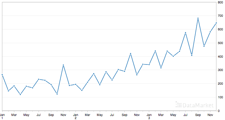
Shampoo Sales Dataset

The dataset shows an increasing trend, and possibly some seasonal component.

Download the dataset and place it in the current working directory with the filename “shampoo-sales.csv“.

Download the dataset.

The following snippet of code will load the Shampoo Sales dataset and plot the time series.

from pandas import read_csv
from pandas import datetime
from matplotlib import pyplot

def parser(x):
	return datetime.strptime('190'+x, '%Y-%m')

series = read_csv('shampoo-sales.csv', header=0, parse_dates=[0], index_col=0, squeeze=True, date_parser=parser)
series.plot()
pyplot.show()

from pandas import read_csv

from pandas import datetime

from matplotlib import pyplot

def parser(x):

return datetime.strptime('190'+x, '%Y-%m')

series = read_csv('shampoo-sales.csv', header=0, parse_dates=[0], index_col=0, squeeze=True, date_parser=parser)

series.plot()

pyplot.show()

Running the example plots the time series, as follows:

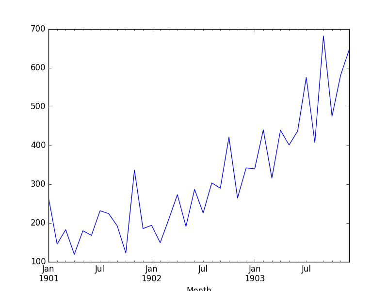
Shampoo Sales Dataset Plot

Persistence Algorithm

A persistence model can be implemented easily in Python.

We will break this section down into 4 steps:

Transform the univariate dataset into a supervised learning problem.
Establish the train and test datasets for the test harness.
Define the persistence model.
Make a forecast and establish a baseline performance.
Review the complete example and plot the output.

Let’s dive in.

Step 1: Define the Supervised Learning Problem

The first step is to load the dataset and create a lagged representation. That is, given the observation at t-1, predict the observation at t+1.

# Create lagged dataset
values = DataFrame(series.values)
dataframe = concat([values.shift(1), values], axis=1)
dataframe.columns = ['t-1', 't+1']
print(dataframe.head(5))

# Create lagged dataset

values = DataFrame(series.values)

dataframe = concat([values.shift(1), values], axis=1)

dataframe.columns = ['t-1', 't+1']

print(dataframe.head(5))

This snippet creates the dataset and prints the first 5 rows of the new dataset.

We can see that the first row (index 0) will have to be discarded as there was no observation prior to the first observation to use to make the prediction.

From a supervised learning perspective, the t-1 column is the input variable, or X, and the t+1 column is the output variable, or y.

     t-1    t+1
0    NaN  266.0
1  266.0  145.9
2  145.9  183.1
3  183.1  119.3
4  119.3  180.3

t-1 t+1

0 NaN 266.0

1 266.0 145.9

2 145.9 183.1

3 183.1 119.3

4 119.3 180.3

Step 2: Train and Test Sets

The next step is to separate the dataset into train and test sets.

We will keep the first 66% of the observations for “training” and the remaining 34% for evaluation. During the split, we are careful to exclude the first row of data with the NaN value.

No training is required in this case; it’s just habit. Each of the train and test sets are then split into the input and output variables.

# split into train and test sets
X = dataframe.values
train_size = int(len(X) * 0.66)
train, test = X[1:train_size], X[train_size:]
train_X, train_y = train[:,0], train[:,1]
test_X, test_y = test[:,0], test[:,1]

# split into train and test sets

X = dataframe.values

train_size = int(len(X) * 0.66)

train, test = X[1:train_size], X[train_size:]

train_X, train_y = train[:,0], train[:,1]

test_X, test_y = test[:,0], test[:,1]

Step 3: Persistence Algorithm

We can define our persistence model as a function that returns the value provided as input.

For example, if the t-1 value of 266.0 was provided, then this is returned as the prediction, whereas the actual real or expected value happens to be 145.9 (taken from the first usable row in our lagged dataset).

# persistence model
def model_persistence(x):
	return x

# persistence model

def model_persistence(x):

return x

Step 4: Make and Evaluate Forecast

Now we can evaluate this model on the test dataset.

We do this using the walk-forward validation method.

No model training or retraining is required, so in essence, we step through the test dataset time step by time step and get predictions.

Once predictions are made for each time step in the training dataset, they are compared to the expected values and a Mean Squared Error (MSE) score is calculated.

# walk-forward validation
predictions = list()
for x in test_X:
	yhat = model_persistence(x)
	predictions.append(yhat)
test_score = mean_squared_error(test_y, predictions)
print('Test MSE: %.3f' % test_score)

# walk-forward validation

predictions = list()

for x in test_X:

yhat = model_persistence(x)

predictions.append(yhat)

test_score = mean_squared_error(test_y, predictions)

print('Test MSE: %.3f' % test_score)

In this case, the error is more than 17,730 over the test dataset.

Test MSE: 17730.518

1	Test MSE: 17730.518

Step 5: Complete Example

Finally, a plot is made to show the training dataset and the diverging predictions from the expected values from the test dataset.

From the plot of the persistence model predictions, it is clear that the model is 1-step behind reality. There is a rising trend and month-to-month noise in the sales figures, which highlights the limitations of the persistence technique.

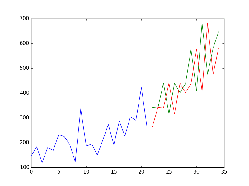
Shampoo Sales Persistence Model

The complete example is listed below.

from pandas import read_csv
from pandas import datetime
from pandas import DataFrame
from pandas import concat
from matplotlib import pyplot
from sklearn.metrics import mean_squared_error

def parser(x):
	return datetime.strptime('190'+x, '%Y-%m')

series = read_csv('shampoo-sales.csv', header=0, parse_dates=[0], index_col=0, squeeze=True, date_parser=parser)
# Create lagged dataset
values = DataFrame(series.values)
dataframe = concat([values.shift(1), values], axis=1)
dataframe.columns = ['t-1', 't+1']
print(dataframe.head(5))

# split into train and test sets
X = dataframe.values
train_size = int(len(X) * 0.66)
train, test = X[1:train_size], X[train_size:]
train_X, train_y = train[:,0], train[:,1]
test_X, test_y = test[:,0], test[:,1]

# persistence model
def model_persistence(x):
	return x

# walk-forward validation
predictions = list()
for x in test_X:
	yhat = model_persistence(x)
	predictions.append(yhat)
test_score = mean_squared_error(test_y, predictions)
print('Test MSE: %.3f' % test_score)

# plot predictions and expected results
pyplot.plot(train_y)
pyplot.plot([None for i in train_y] + [x for x in test_y])
pyplot.plot([None for i in train_y] + [x for x in predictions])
pyplot.show()

from pandas import read_csv

from pandas import datetime

from pandas import DataFrame

from pandas import concat

from matplotlib import pyplot

from sklearn.metrics import mean_squared_error

def parser(x):

return datetime.strptime('190'+x, '%Y-%m')

series = read_csv('shampoo-sales.csv', header=0, parse_dates=[0], index_col=0, squeeze=True, date_parser=parser)

# Create lagged dataset

values = DataFrame(series.values)

dataframe = concat([values.shift(1), values], axis=1)

dataframe.columns = ['t-1', 't+1']

print(dataframe.head(5))

# split into train and test sets

X = dataframe.values

train_size = int(len(X) * 0.66)

train, test = X[1:train_size], X[train_size:]

train_X, train_y = train[:,0], train[:,1]

test_X, test_y = test[:,0], test[:,1]

# persistence model

def model_persistence(x):

return x

# walk-forward validation

predictions = list()

for x in test_X:

yhat = model_persistence(x)

predictions.append(yhat)

test_score = mean_squared_error(test_y, predictions)

print('Test MSE: %.3f' % test_score)

# plot predictions and expected results

pyplot.plot(train_y)

pyplot.plot([None for i in train_y] + [x for x in test_y])

pyplot.plot([None for i in train_y] + [x for x in predictions])

pyplot.show()

We have seen an example of the persistence model developed from scratch for the Shampoo Sales problem.

The persistence algorithm is naive. It is often called the naive forecast.

It assumes nothing about the specifics of the time series problem to which it is applied. This is what makes it so easy to understand and so quick to implement and evaluate.

As a machine learning practitioner, it can also spark a large number of improvements.

Write them down.

This is useful because these ideas can become input features in a feature engineering effort or simple models that may be combined in an ensembling effort later.

Summary

In this tutorial, you discovered how to establish a baseline performance on time series forecast problems with Python.

Specifically, you learned:

The importance of establishing a baseline and the persistence algorithm that you can use.
How to implement the persistence algorithm in Python from scratch.
How to evaluate the forecasts of the persistence algorithm and use them as a baseline.

Do you have any questions about baseline performance, or about this tutorial?
Ask your questions in the comments below and I will do my best to answer.

84 Responses to How to Make Baseline Predictions for Time Series Forecasting with Python

Kevin December 26, 2016 at 3:56 pm #

Great post. However, I think instead of (t-1) and (t+1), it should be (t) and (t+1). The former indicates a lag of 2 time steps; the persistence model only requires a 1 step look-back.

Reply
- Jason Brownlee December 27, 2016 at 5:21 am #
  
  That would be clearer, thanks Kevin.
  
  Reply
- Hans April 26, 2017 at 7:05 pm #
  
  Any suggestion how to implement this?
  
  Reply
  - Hans April 27, 2017 at 6:17 pm #
    
    Is it only a question of column declarations?
    
    dataframe.columns = [‘t-1’, ‘t+1’] vs. dataframe.columns = [‘t’, ‘t+1’]
    
    …or do I have to change some more code logic?
    
    Reply
Ansh Gandhi December 27, 2016 at 9:30 am #

Great post!

Reply
- Jason Brownlee December 28, 2016 at 7:01 am #
  
  Thanks Ansh.
  
  Reply
electricscootershq.org December 28, 2016 at 9:33 am #

Creating a forecast for a baseline. The hard part of baselines is, of course, the future. How good are economists or meteorologists at predicting the stock market or weather? Uncertainty is an unavoidable part of this part of the work.

Reply
- Jason Brownlee December 29, 2016 at 7:14 am #
  
  Yes, not sure I follow. Perhaps you could restate your point?
  
  Reply
Hans April 26, 2017 at 6:37 pm #

Hello, I have a question.

Quote: “If a model achieves performance at or below the baseline,
..the technique should be fixed or abandoned”

Where is the baseline in the plot?

What does it mean at or below the baseline in regard of the example plots?

What does the red and the green line describe?

I assume:

blue line = training data
green line = test data
red line = prediction

Am I right?

I’m not afraid to ask stupid questions. I’ve studied a lot and know no one knows everything :-).

Reply
- Jason Brownlee April 27, 2017 at 8:37 am #
  
  Here, baseline is the model you have chosen to be the baseline. E.g. a persistence forecast.
  
  Reply
  - Hans April 27, 2017 at 6:06 pm #
    
    So then I have to compare the MSE-values of the baseline model and a chosen model
    to decide whether my chosen model is the right model to predict something.
    
    The performance of the baseline model is:
    
    Test Score: 17730.518 MSE
    
    I have feeded the shampoo-data into your Multilayer Perceptron-example.
    
    Test A)
    
    The performance of the Multilayer Perceptron Model on the shampoo-data is:
    
    Train Score: 6623.57 MSE
    
    Test Score: 19589.78 MSE
    
    Test Score mlp model: 19589.78 MSE > Test Score baseline model: 17730.518 MSE
    
    Conclusion:
    
    The choosen mlp model predicts something, because its MSE is higher then
    the MSE of the baseline model while using the same raw data.
    ‘There is some significance’.
    
    Is this right so far?
    Actually I would expect I higher error rate as bad sign.
    
    Test B)
    Airline LSTM Example (feeded with shampoo data):
    
    testScoreMyTest = mean_squared_error(testY[0], testPredict[:,0])
    print(‘testScoreMyTest: %.2f MSE’ % (testScoreMyTest))
    
    Test Score Airline LSTM: 20288.20 MSE > Test Score baseline model: 17730.518 MSE
    
    Conclusion:
    
    Airline LSTM Example predicts something on shampoo data.
    Here I have a problem. I wanted to see if user Wollner is right.
    https://machinelearningmastery.com/time-series-prediction-lstm-recurrent-neural-networks-python-keras/#comment-383708
    
    Does the baseline test shows that he isn’t right???
    
    Reply
    - Hans April 27, 2017 at 6:51 pm #
      
      I also try it with RMSE
      
      testScore = math.sqrt(mean_squared_error(test_y, predictions))
      print(‘Test Score: %.2f RMSE’ % (testScore))
      
      The smaller the value of the RMSE, the better is the predictive accuracy of the model.
      
      http://docs.aws.amazon.com/machine-learning/latest/dg/regression-model-insights.html
      
      The performance of the baseline model is:
      
      testScore = math.sqrt(mean_squared_error(test_y, predictions))
      print(‘Test Score: %.2f RMSE’ % (testScore))
      
      Test Score: 133.16 RMSE
      
      I have feeded the shampoo-data into your Multilayer Perceptron-example.
      
      Test A)
      The performance of the Multilayer Perceptron Model on the shampoo-data is:
      
      Test Score: 139.96 RMSE > 133.16 RMSE
      
      Test B)
      Airline LSTM Example (feeded with shampoo data):
      
      Test Score: 142.43 RMSE > 133.16 RMSE
      
      Conclusion:
      
      Actually in regard to the Amazon documentation, I would say both models
      perform bad compared to the baseline model and therefore they
      are NOT professionally qualified to solve the ‘shampoo problem’.
      
      Do I have a misconception here?
      
      Reply
    - Jason Brownlee April 28, 2017 at 7:37 am #
      
      The idea is to compare the performance of the baseline model to all other models that you evaluate on your problem.
      
      Regarding MSE, the goal is to minimize the error, so smaller values are better.
      
      Reply
Hans April 26, 2017 at 6:52 pm #

I try to use labels in the plot according to http://matplotlib.org/users/legend_guide.html

Example:

pyplot.plot(train_y, label=’Training Data’)

But every time I have to go to options in the plot window and check auto generate labels to view my declarations.

Is this behavior normal?

Reply
- Jason Brownlee April 27, 2017 at 8:38 am #
  
  I am not an expert in matplotlib sorry, but you can style everything about your plots programmatically.
  
  Reply
Vlad December 10, 2017 at 2:20 am #

great post, read the whole mini course and i’m now trying to implement it.

any tips on modifying the code to accept multivariate inputs?

Reply
- Jason Brownlee December 10, 2017 at 5:21 am #
  
  Thanks.
  
  I hope to cover multivariate cases in more detail in the future.
  
  Reply
Howell December 12, 2017 at 10:12 am #

Why is there a gap in the persistence model graph in step 5? how to close that gap in graph?

Reply
- Jason Brownlee December 12, 2017 at 4:08 pm #
  
  Not sure I follow?
  
  We are plotting different series so they start and end at different places and have different colors.
  
  I guess you can plot whatever you like, such as concatenate the history with the predictions?
  
  Reply
Aditya Sharma April 18, 2018 at 9:05 pm #

Hey Jason
Can you tell how can we get the next month’s forecasted value?
lets say i have a data of n months then how t predict what will be its value in n+1 month?

Reply
- Jason Brownlee April 19, 2018 at 6:31 am #
  
  Yes, see this post:
  https://machinelearningmastery.com/make-sample-forecasts-arima-python/
  
  Reply
Ankit Tripathi May 21, 2018 at 5:30 pm #

Hey Jason,

Is there a way so set cap and floor while forecasting through ARIMA? It would be useful to avoid erroneous values for a business data.

Reply
- Jason Brownlee May 22, 2018 at 6:23 am #
  
  You can post-process the forecast prior to evaluation.
  
  Reply
  - Ankit Tripathi May 23, 2018 at 3:26 am #
    
    Yeah I did that. I thought, may be there is a way to pass the bounds as parameters like its possible in Prophet in R. Anyway, thanks Jason 🙂
    
    Reply
Andrea June 21, 2018 at 5:41 pm #

Hi, Thank you for your good posting! 😀

I read a lot of your articles. I have question, though.

Making predictions, using LSTM, on random walk process(= like stock price) results in baseline prediction.

How can I evade this?

Any suggestions would helpful. Thank you!

Reply
- Jason Brownlee June 22, 2018 at 6:02 am #
  
  Some problems are not predictable, e.g. those that are a random walk.
  
  Reply
KR Ju July 14, 2018 at 7:04 pm #

thanks for your blog, Jason.
even after readied this article, I don’t understand it fully.
according to you, persistence model is not forecasting. the word “prediction” could be not suitable in this topic, isn’t it?

Could you tell; when I obtained a fully matched persistence plot with the raw data plot, what does mean that?
Ju

Reply
- Jason Brownlee July 15, 2018 at 6:10 am #
  
  It is a prediction, just a naive prediction.
  
  Reply
KR Ju July 14, 2018 at 7:08 pm #

Jason, furthermore in this blog,

if I got the completely matched baseline with the raw data plot, I don’t need to apply other models for solving the targeted problem?

Ju

Reply
- Jason Brownlee July 15, 2018 at 6:11 am #
  
  If the persistence model gives zero error, it means your time series is a flat straight line (e.g. has no information).
  
  Otherwise, perhaps you have a bug?
  
  Reply
Brian Stephans August 7, 2018 at 4:49 am #

Hello Dr,

I am having to problem with loading the data, It seems I always have issues with data with datetime but cant seem to figure out the issue, I am new to python. hopefully you can help me out as I am loving your website. It seems that the error is in line 6

/usr/local/bin/python3.7 /Users/Brian/PycharmProjects/MachineLearningMasteryTimeSeries1/baselinezerorule.py
Traceback (most recent call last):
File “/Library/Frameworks/Python.framework/Versions/3.7/lib/python3.7/site-packages/pandas/io/parsers.py”, line 3021, in converter
date_parser(*date_cols), errors=’ignore’)
File “/Users/Brian/PycharmProjects/MachineLearningMasteryTimeSeries1/baselinezerorule.py”, line 6, in parser
return datetime.strptime(‘190 ‘ +x, ‘%Y-%m’)
TypeError: strptime() argument 1 must be str, not numpy.ndarray

During handling of the above exception, another exception occurred:

Traceback (most recent call last):
File “/Library/Frameworks/Python.framework/Versions/3.7/lib/python3.7/site-packages/pandas/io/parsers.py”, line 3030, in converter
dayfirst=dayfirst),
File “pandas/_libs/tslibs/parsing.pyx”, line 434, in pandas._libs.tslibs.parsing.try_parse_dates
File “pandas/_libs/tslibs/parsing.pyx”, line 431, in pandas._libs.tslibs.parsing.try_parse_dates
File “/Users/Brian/PycharmProjects/MachineLearningMasteryTimeSeries1/baselinezerorule.py”, line 6, in parser
return datetime.strptime(‘190 ‘ +x, ‘%Y-%m’)
File “/Library/Frameworks/Python.framework/Versions/3.7/lib/python3.7/_strptime.py”, line 577, in _strptime_datetime
tt, fraction, gmtoff_fraction = _strptime(data_string, format)
File “/Library/Frameworks/Python.framework/Versions/3.7/lib/python3.7/_strptime.py”, line 359, in _strptime
(data_string, format))
ValueError: time data ‘190 1-01’ does not match format ‘%Y-%m’

During handling of the above exception, another exception occurred:

Traceback (most recent call last):
File “/Users/Brian/PycharmProjects/MachineLearningMasteryTimeSeries1/baselinezerorule.py”, line 8, in
series = read_csv(‘shampoo-sales.csv’, header=0, parse_dates=[0], index_col=0, squeeze=True, date_parser=parser)
File “/Library/Frameworks/Python.framework/Versions/3.7/lib/python3.7/site-packages/pandas/io/parsers.py”, line 678, in parser_f
return _read(filepath_or_buffer, kwds)
File “/Library/Frameworks/Python.framework/Versions/3.7/lib/python3.7/site-packages/pandas/io/parsers.py”, line 446, in _read
data = parser.read(nrows)
File “/Library/Frameworks/Python.framework/Versions/3.7/lib/python3.7/site-packages/pandas/io/parsers.py”, line 1036, in read
ret = self._engine.read(nrows)
File “/Library/Frameworks/Python.framework/Versions/3.7/lib/python3.7/site-packages/pandas/io/parsers.py”, line 1922, in read
index, names = self._make_index(data, alldata, names)
File “/Library/Frameworks/Python.framework/Versions/3.7/lib/python3.7/site-packages/pandas/io/parsers.py”, line 1426, in _make_index
index = self._agg_index(index)
File “/Library/Frameworks/Python.framework/Versions/3.7/lib/python3.7/site-packages/pandas/io/parsers.py”, line 1504, in _agg_index
arr = self._date_conv(arr)
File “/Library/Frameworks/Python.framework/Versions/3.7/lib/python3.7/site-packages/pandas/io/parsers.py”, line 3033, in converter
return generic_parser(date_parser, *date_cols)
File “/Library/Frameworks/Python.framework/Versions/3.7/lib/python3.7/site-packages/pandas/io/date_converters.py”, line 39, in generic_parser
results[i] = parse_func(*args)
File “/Users/Brian/PycharmProjects/MachineLearningMasteryTimeSeries1/baselinezerorule.py”, line 6, in parser
return datetime.strptime(‘190 ‘ +x, ‘%Y-%m’)
File “/Library/Frameworks/Python.framework/Versions/3.7/lib/python3.7/_strptime.py”, line 577, in _strptime_datetime
tt, fraction, gmtoff_fraction = _strptime(data_string, format)
File “/Library/Frameworks/Python.framework/Versions/3.7/lib/python3.7/_strptime.py”, line 359, in _strptime
(data_string, format))
ValueError: time data ‘190 1-01’ does not match format ‘%Y-%m’

Process finished with exit code 1

Reply
- Jason Brownlee August 7, 2018 at 6:34 am #
  
  It may be the version of the dataset that you have downloaded.
  
  I have a copy of the datasets ready to use here:
  https://github.com/jbrownlee/Datasets
  
  Reply
András Novoszáth October 9, 2018 at 1:47 am #

Hi, great post, I was just wondering why do we need the for loop for calculating predictions and then the error rate, when it seems to me that we could simply use the following line:

test_score = mean_squared_error(test_y, test_X)

Do I miss something?

Reply
- Jason Brownlee October 9, 2018 at 8:46 am #
  
  It was more the methodology, you can substitute the persistance forecast for whatever you like.
  
  Reply
Hossein March 12, 2019 at 3:14 pm #

But I think it’s not just about being clearer. t-1 is totally wrong and it should be t. Thanks Jason!

Reply
Leen April 1, 2019 at 3:38 pm #

Hello Jason, Thank you for the awesome tutorials!!

Can we make persistence models for multivariate time series ??

Reply
- Jason Brownlee April 2, 2019 at 8:03 am #
  
  Yes.
  
  Reply
  - Leen April 3, 2019 at 10:25 pm #
    
    but by doing that, we take only the target column and discard all others right ?
    
    Reply
    - Jason Brownlee April 4, 2019 at 7:57 am #
      
      Yes, that is correct.
      
      Reply
Amin April 7, 2019 at 3:04 am #

Thanks for the nice work, Do you find out that the model is stationary only by looking at the graph? It is mentioned that data shows possibly some seasonal component? Do we need to confirm this?

Reply
- Jason Brownlee April 7, 2019 at 5:34 am #
  
  You can use a statistical test to check if the time series is stationary:
  https://machinelearningmastery.com/time-series-data-stationary-python/
  
  Reply
Lhicel Joyce Aytona April 27, 2019 at 4:50 am #

What if machine learning cannot beat RMSE of persistence model (uses t-1 data for t+1 prediction)? What can we do to improve model? or maybe other ways of measuring predictive capability of model?

Reply
- Jason Brownlee April 27, 2019 at 6:37 am #
  
  It is possible that your time series is not predictable.
  
  Try exhausting the ideas on this list:
  https://machinelearningmastery.com/machine-learning-performance-improvement-cheat-sheet/
  
  Reply
Claire Taylor May 25, 2019 at 3:03 pm #

Hi Jason, I’m wondering why predicted model looks shifted one step from the test data? It looks like our model a lil bit late from the real observations. So how to correct it? Thanks in advance.

Reply
- Jason Brownlee May 26, 2019 at 6:40 am #
  
  That is called a persistence model and its the simplest time series forecasting method to use and compare to more advanced methods.
  
  Reply
  - Louiza January 11, 2023 at 3:46 am #
    
    Thank you for your amazing articles. They are so much helpful.
    I am trying to apply a pytorch forecasting baseline on my timeseries data(solar irradiance). The mse equals or near zero when I try to forecast less than 8h however it’s above 100 when I do otherwise.
    Is this normal??
    And
    What kind of baseline does pytorch forecasting uses.
    
    Reply
    - James Carmichael January 11, 2023 at 7:56 am #
      
      Hi Louiza…You are very welcome!
      
      You may be working on a regression problem and achieve zero prediction errors.
      
      Alternately, you may be working on a classification problem and achieve 100% accuracy.
      
      This is unusual and there are many possible reasons for this, including:
      
      You are evaluating model performance on the training set by accident.
      Your hold out dataset (train or validation) is too small or unrepresentative.
      You have introduced a bug into your code and it is doing something different from what you expect.
      Your prediction problem is easy or trivial and may not require machine learning.
      The most common reason is that your hold out dataset is too small or not representative of the broader problem.
      
      This can be addressed by:
      
      Using k-fold cross-validation to estimate model performance instead of a train/test split.
      Gather more data.
      Use a different split of data for train and test, such as 50/50.
      
      Reply
Ruth July 24, 2019 at 6:58 am #

Hi Jason – I’m really enjoying these tutorials! Very informative. One problem – I keep getting stuck at the walk-forward validation part of all the exercises. When I execute the code “test_score = mean_squared_error(test_y, predictions)” I keep getting the following error:

“Found input variables with inconsistent numbers of samples”

Any suggestions on how to troubleshoot? I’ve had the same error message for the shampoo, champagne, and daily births datasets. Thank you so much for your help!

Reply
- Jason Brownlee July 24, 2019 at 8:20 am #
  
  It might suggest that the number of examples in test_y and predictions don’t match.
  
  Perhaps bug crept in to your example?
  
  Reply
- Girish LC August 7, 2020 at 12:57 pm #
  
  train_X, train_y = train[:,0], train[:,1]
  test_X, test_y = test[:,0], test[:,1]
  
  Reply
thiagu October 1, 2019 at 1:49 pm #

hi jason,
i have little confusion about walk forward validation and persistence model …i couldnt understand the purpose.. could you give me clear idea..

Reply
- Jason Brownlee October 1, 2019 at 2:19 pm #
  
  You can learn more about walk forward validation here:
  https://machinelearningmastery.com/backtest-machine-learning-models-time-series-forecasting/
  
  Reply
thiagu October 1, 2019 at 4:17 pm #

hi jason ,
can i use walk forward validation in multivariate time series data…

Reply
- Jason Brownlee October 2, 2019 at 7:49 am #
  
  Yes, you can discover many examples here:
  https://machinelearningmastery.com/start-here/#deep_learning_time_series
  
  Reply
thiagu October 3, 2019 at 12:51 am #

Thank u…

Reply
- Jason Brownlee October 3, 2019 at 6:50 am #
  
  You’re welcome!
  
  Reply
Tom Leung February 16, 2020 at 7:20 pm #

Hi Jason,

Thanks for your great post on time series forecasting!

I want to do multi-step forecasting, what would be a good choice of baseline model? If I don’t get it wrong, the persistence model just copies the value of time t-1 as the prediction of time t, it will be a straight line when predicting multiple steps.

Thanks!

Reply
- Jason Brownlee February 17, 2020 at 7:43 am #
  
  Persistance is a great baseline model for one-step and multi-step forecasting.
  
  Reply
  - Eduardo July 31, 2020 at 11:41 am #
    
    Let me understand, you created a persistance model, what is framed the problem as supervised problem and see the performance, so what is the best option to address this problem?
    This is having just inputs (x) and predicting (y) or what is the best option?
    
    Reply
    - Jason Brownlee July 31, 2020 at 1:41 pm #
      
      Sorry, I don’t understand your question, can you please elaborate or restate it?
      
      Reply
Nicholas Jallan April 6, 2020 at 6:06 pm #

Hi Jason,

There’s something to me that seems deeply wrong : you do your prediction with the test data… it should be done from training data… test data should be used as ground truth and comparison with the forecast.
Right now, as is, all you do is just a shifted copy paste of your values. It’s useless and certainly not a forecast in any way.

Reply
- Jason Brownlee April 7, 2020 at 5:43 am #
  
  It can be confusing when you’re new to time series.
  
  We use-walk forward validation to evaluate the model – you can learn more about here:
  https://machinelearningmastery.com/backtest-machine-learning-models-time-series-forecasting/
  
  Reply
Girish LC August 7, 2020 at 12:36 pm #

Hi Jason,

Thank you very much for the wonderful explanation, I become fan of you.

Can you please provide me the link to handle multivariate forecasting.

Question: So for the same dataset if we build any other model, the MSE value should be less than 17,730. Am I right ?

Reply
- Jason Brownlee August 7, 2020 at 1:31 pm #
  
  You’re welcome.
  
  Yes, there are 100s on the blog, start here:
  https://machinelearningmastery.com/start-here/#deep_learning_time_series
  
  A skilful model must out-perform persistence.
  
  Reply
  - Girish LC August 10, 2020 at 8:20 pm #
    
    Thank you Jason.
    
    Reply
    - Jason Brownlee August 11, 2020 at 6:30 am #
      
      You’re welcome.
      
      Reply
Priya October 8, 2020 at 8:29 pm #

Hi, Is it necessary to apply baseline model (for ex persistence) on raw data or can we apply differencing or normalization before applying persistence model

Reply
- Priya October 8, 2020 at 8:47 pm #
  
  Actually in my case Persistence model on raw data is giving terrible results with negative r2-score. But when I am applying seasonal differencing with persistence model then it is giving very good results.
  
  Please give me suggestion that why it is happening and what should I do?
  
  Reply
  - Jason Brownlee October 9, 2020 at 6:44 am #
    
    You can use a persistance model with seasonal differencing as the baseline if you wish. It’s your project!
    
    Reply
- Jason Brownlee October 9, 2020 at 6:43 am #
  
  Yes, the baseline should make no/few assumptions and operate on the raw data.
  
  Reply
pals October 29, 2020 at 7:25 pm #

Hi,
I need to use Moving average (with windows of 3 , 7 and 30 )and then calculate the MAE and rmse ?
How do I do that . Also where does shift(1) and walk forward fit into this ?
is shift(1) same as windows = 1 of Moving average ?

Reply
- Jason Brownlee October 30, 2020 at 6:49 am #
  
  This will help you to prepare your data:
  https://machinelearningmastery.com/time-series-forecasting-supervised-learning/
  
  Reply
Ben Bartling December 3, 2020 at 7:57 am #

Hi Jason,

If your project was forecasting out 24 samples at a time. Hourly data one day look a head’s. Could you ever make a persistence model that reflects that process? Not one data sample at a time, but 24 samples at a time.

For example, for each day in my test dataset (~ half year) my persistence model will forecast out 24 samples at a time which would be yesterdays data (24 samples)

Hopefully that makes sense. I think i could then compare this persistence model results RMSE to my actual ML timeseries forecasting RMSE of the same test dataset for one day look ahead results … right?

Reply
- Jason Brownlee December 3, 2020 at 8:25 am #
  
  Sure, I think you’re describing multi-step forecasting, e.g. input some number of time steps and predict some number of time steps (7 days, 24 hours, 10 minutes, etc.) There are many many examples on the blog.
  
  Reply
Qizal Ashfaq March 24, 2021 at 10:26 am #

Can persistence model do multistep forecasting? How to use this as a baseline model for multivariate multistep forecasting ?

Reply
- Jason Brownlee March 25, 2021 at 4:37 am #
  
  Sure, take the last value of each variable and use them for each forecast step.
  
  Reply
Paul Holdsworth July 12, 2021 at 11:08 am #

Hi Jason,

What is the purpose of ‘190+x’ in:

return datetime.strptime(‘190’+x, ‘%Y-%m’)?

Thanks

Reply
- Jason Brownlee July 13, 2021 at 5:14 am #
  
  To parse the date in the data correctly.
  
  Reply
Victor August 5, 2021 at 9:37 pm #

Hi Jason, thank you for articles – for this one and for the plenty of others!

Just minor remark:

from pandas import datetime – caused the warning
“FutureWarning: The pandas.datetime class is deprecated and will be removed from pandas in a future version. Import from datetime module instead.”

So, in my code i’ve changed it as recommended
import datetime as dt

Reply
- Jason Brownlee August 6, 2021 at 4:56 am #
  
  Thanks!
  
  Reply
Huy Truong March 8, 2022 at 7:16 am #

Hi Jason, can you explain your following conclusion, “There is a rising trend and month-to-month noise in the sales figures, which highlights the limitations of the persistence technique.”

I’m not sure about the “month-to-month noise”

— Thanks!

Reply
- James Carmichael March 9, 2022 at 6:00 am #
  
  Hi Huy…The following may be of interest to you:
  
  https://machinelearningmastery.com/decompose-time-series-data-trend-seasonality/
  
  Reply
nate April 3, 2022 at 8:14 am #

i am not too sure what you mean by “No model training or retraining is required, so in essence, we step through the test dataset time step by time step and get predictions.” what is the point of spliting the data into train and test, if train is not used for model. From what i read on this topic, am i right to say that the goal is for doing all this is for getting the mean squared error which can be used as a baseline for model selection?

Reply
- James Carmichael April 3, 2022 at 10:32 am #
  
  Hi Nate…If possible you should have separate, training, testing and validation datasets.
  
  Reply

Navigation

How to Make Baseline Predictions for Time Series Forecasting with Python

Forecast Performance Baseline

Stop learning Time Series Forecasting the slow way!

Persistence Algorithm (the “naive” forecast)

Shampoo Sales Dataset

Persistence Algorithm

Step 1: Define the Supervised Learning Problem

Step 2: Train and Test Sets

Step 3: Persistence Algorithm

Step 4: Make and Evaluate Forecast

Step 5: Complete Example

Summary

Want to Develop Time Series Forecasts with Python?

Develop Your Own Forecasts in Minutes

Finally Bring Time Series Forecasting to
Your Own Projects

More On This Topic

84 Responses to How to Make Baseline Predictions for Time Series Forecasting with Python

Leave a Reply Click here to cancel reply.

Navigation

Forecast Performance Baseline

Stop learning Time Series Forecasting the slow way!

Persistence Algorithm (the “naive” forecast)

Shampoo Sales Dataset

Persistence Algorithm

Step 1: Define the Supervised Learning Problem

Step 2: Train and Test Sets

Step 3: Persistence Algorithm

Step 4: Make and Evaluate Forecast

Step 5: Complete Example

Summary

Want to Develop Time Series Forecasts with Python?

Develop Your Own Forecasts in Minutes

Finally Bring Time Series Forecasting to Your Own Projects

More On This Topic

84 Responses to How to Make Baseline Predictions for Time Series Forecasting with Python

Leave a Reply Click here to cancel reply.

Finally Bring Time Series Forecasting to
Your Own Projects