Overfitting is a problem with sophisticated non-linear learning algorithms like gradient boosting.
In this post you will discover how you can use early stopping to limit overfitting with XGBoost in Python.
After reading this post, you will know:
About early stopping as an approach to reducing overfitting of training data.
How to monitor the performance of an XGBoost model during training and plot the learning curve.
How to use early stopping to prematurely stop the training of an XGBoost model at an optimal epoch.
Kick-start your project with my new book XGBoost With Python, including step-by-step tutorials and the Python source code files for all examples.
Let’s get started.
Update Jan/2017: Updated to reflect changes in scikit-learn API version 0.18.1.
Update Mar/2018: Added alternate link to download the dataset as the original appears to have been taken down.
Avoid Overfitting By Early Stopping With XGBoost In Python Photo by Michael Hamann, some rights reserved.
Need help with XGBoost in Python?
Take my free 7-day email course and discover xgboost (with sample code).
Click to sign-up now and also get a free PDF Ebook version of the course.
Early Stopping to Avoid Overfitting
Early stopping is an approach to training complex machine learning models to avoid overfitting.
It works by monitoring the performance of the model that is being trained on a separate test dataset and stopping the training procedure once the performance on the test dataset has not improved after a fixed number of training iterations.
It avoids overfitting by attempting to automatically select the inflection point where performance on the test dataset starts to decrease while performance on the training dataset continues to improve as the model starts to overfit.
The performance measure may be the loss function that is being optimized to train the model (such as logarithmic loss), or an external metric of interest to the problem in general (such as classification accuracy).
Monitoring Training Performance With XGBoost
The XGBoost model can evaluate and report on the performance on a test set for the the model during training.
It supports this capability by specifying both an test dataset and an evaluation metric on the call to model.fit() when training the model and specifying verbose output.
For example, we can report on the binary classification error rate (“error“) on a standalone test set (eval_set) while training an XGBoost model as follows:
Running this example trains the model on 67% of the data and evaluates the model every training epoch on a 33% test dataset.
The classification error is reported each iteration and finally the classification accuracy is reported at the end.
Note: Your results may vary given the stochastic nature of the algorithm or evaluation procedure, or differences in numerical precision. Consider running the example a few times and compare the average outcome.
The output is provided below, truncated for brevity. We can see that the classification error is reported each training iteration (after each boosted tree is added to the model).
1
2
3
4
5
6
7
8
9
10
11
12
13
...
[89] validation_0-error:0.204724
[90] validation_0-error:0.208661
[91] validation_0-error:0.208661
[92] validation_0-error:0.208661
[93] validation_0-error:0.208661
[94] validation_0-error:0.208661
[95] validation_0-error:0.212598
[96] validation_0-error:0.204724
[97] validation_0-error:0.212598
[98] validation_0-error:0.216535
[99] validation_0-error:0.220472
Accuracy: 77.95%
Reviewing all of the output, we can see that the model performance on the test set sits flat and even gets worse towards the end of training.
Evaluate XGBoost Models With Learning Curves
We can retrieve the performance of the model on the evaluation dataset and plot it to get insight into how learning unfolded while training.
We provide an array of X and y pairs to the eval_metric argument when fitting our XGBoost model. In addition to a test set, we can also provide the training dataset. This will provide a report on how well the model is performing on both training and test sets during training.
In addition, the performance of the model on each evaluation set is stored and made available by the model after training by calling the model.evals_result() function. This returns a dictionary of evaluation datasets and scores, for example:
1
2
results=model.evals_result()
print(results)
This will print results like the following (truncated for brevity):
Each of ‘validation_0‘ and ‘validation_1‘ correspond to the order that datasets were provided to the eval_set argument in the call to fit().
A specific array of results, such as for the first dataset and the error metric can be accessed as follows:
1
results['validation_0']['error']
Additionally, we can specify more evaluation metrics to evaluate and collect by providing an array of metrics to the eval_metric argument of the fit() function.
We can then use these collected performance measures to create a line plot and gain further insight into how the model behaved on train and test datasets over training epochs.
Below is the complete code example showing how the collected results can be visualized on a line plot.
1
2
3
4
5
6
7
8
9
10
11
12
13
14
15
16
17
18
19
20
21
22
23
24
25
26
27
28
29
30
31
32
33
34
35
36
37
38
39
40
41
42
43
# plot learning curve
from numpy import loadtxt
from xgboost import XGBClassifier
from sklearn.model_selection import train_test_split
Running this code reports the classification error on both the train and test datasets each epoch. We can turn this off by setting verbose=False (the default) in the call to the fit() function.
Note: Your results may vary given the stochastic nature of the algorithm or evaluation procedure, or differences in numerical precision. Consider running the example a few times and compare the average outcome.
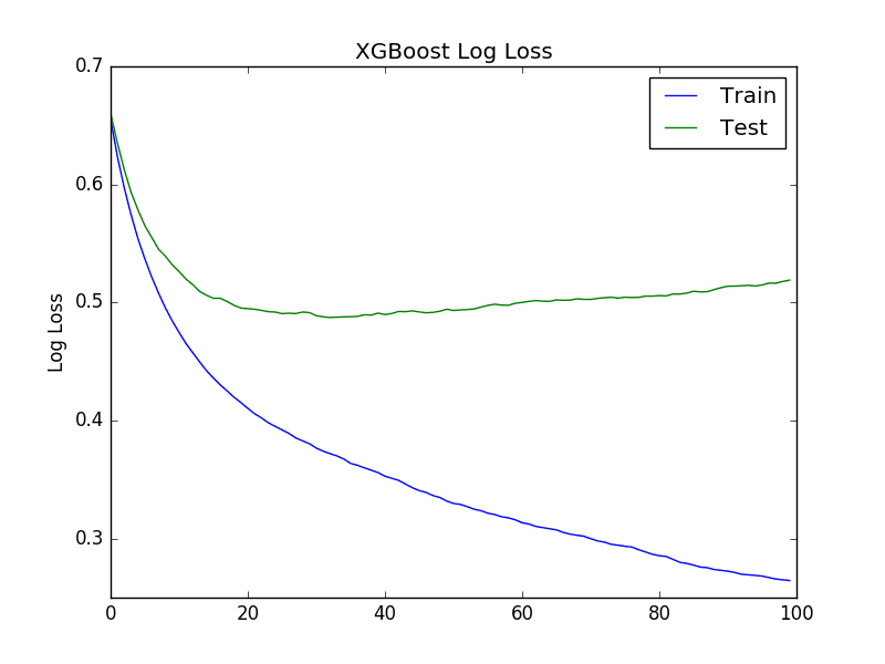
Two plots are created. The first shows the logarithmic loss of the XGBoost model for each epoch on the training and test datasets.
XGBoost Learning Curve Log Loss
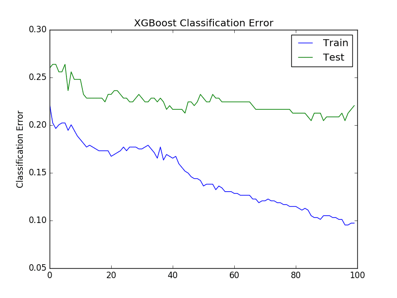
The second plot shows the classification error of the XGBoost model for each epoch on the training and test datasets.
XGBoost Learning Curve Classification Error
From reviewing the logloss plot, it looks like there is an opportunity to stop the learning early, perhaps somewhere around epoch 20 to epoch 40.
We see a similar story for classification error, where error appears to go back up at around epoch 40.
Early Stopping With XGBoost
XGBoost supports early stopping after a fixed number of iterations.
In addition to specifying a metric and test dataset for evaluation each epoch, you must specify a window of the number of epochs over which no improvement is observed. This is specified in the early_stopping_rounds parameter.
For example, we can check for no improvement in logarithmic loss over the 10 epochs as follows:
Note: Your results may vary given the stochastic nature of the algorithm or evaluation procedure, or differences in numerical precision. Consider running the example a few times and compare the average outcome.
Running the example provides the following output, truncated for brevity.
1
2
3
4
5
6
7
8
9
10
11
...
[35] validation_0-logloss:0.487962
[36] validation_0-logloss:0.488218
[37] validation_0-logloss:0.489582
[38] validation_0-logloss:0.489334
[39] validation_0-logloss:0.490969
[40] validation_0-logloss:0.48978
[41] validation_0-logloss:0.490704
[42] validation_0-logloss:0.492369
Stopping. Best iteration:
[32] validation_0-logloss:0.487297
We can see that the model stopped training at epoch 42 (close to what we expected by our manual judgment of learning curves) and that the model with the best loss was observed at epoch 32.
It is generally a good idea to select the early_stopping_rounds as a reasonable function of the total number of training epochs (10% in this case) or attempt to correspond to the period of inflection points as might be observed on plots of learning curves.
Summary
In this post you discovered about monitoring performance and early stopping.
You learned:
About the early stopping technique to stop model training before the model overfits the training data.
How to monitor the performance of XGBoost models during training and to plot learning curves.
How to configure early stopping when training XGBoost models.
Do you have any questions about overfitting or about this post? Ask your questions in the comments and I will do my best to answer.
1. What should we do if the error on train is higher as compared to error on test.
2. Apart for ealry stopping how can we tune regularization parameters effectively ?
Interesting question. Ideally, we want the error on train and test to be good. Generally, error on train is a little lower than test. If it is the other way around it might be a fluke and a sign of underlearning.
Hi Jason,
Thank you for this post, it is very handy and clear.
In the case that I have a task that is measured by another metric, as F-score, will we find the optimal epoch in the loss learning curve or in this new metric? Are there proportional, even with Accuracy?
Hi Jason
Thanks for your sharing!
I have a question that since the python API document mention that
Early stopping returns the model from the last iteration (not the best one). If early stopping occurs, the model will have three additional fields: bst.best_score, bst.best_iteration and bst.best_ntree_limit.
So the model we get when early stopping occur may not be the best model, right?
how can we get that best model?
The best model is in fact used by default when the predict method of the xgb estimator is called. The documentation of that method states:
“ntree_limit (int) – Limit number of trees in the prediction; defaults to best_ntree_limit if defined (i.e. it has been trained with early stopping), otherwise 0 (use all trees).”
You’ve selected early stopping rounds = 10, but why did the total epochs reached 42. Since you said the best may not be the best, then how do i get to control the number of epochs in my final model?
I have a question regarding the use of the test set for early stopping to avoid overfitting…
Shouldn’t you use the train set? Shouldn’t we use the test set only for testing the model and not for optimizing it? (I see early stopping as model optimization)
I thought we would stop when the performances on the training set don’t improve in xx rounds to avoid to create a lot of not useful trees. Then use the selected number of estimator to compute the performances on the test set. Otherwise we might risk to evaluate our model using overoptimistic results. ie. we might get very high AUC because we select the best model, but in a real world experiment where we do not have labels our performances will decrease a lot. The use of the earlystopping on the evaluation set is legitim.. Could you please elaborate and give your opinion?
In short my point is: how can we use the early stopping on the test set if (in principle) we should use the labels of the test set only to evaluate the results of our model and not to “train/optimize” further the model…
I totally agree with G according to my experience. Jason, I think that the example using the test set for both early stopping and prediction is not correct.
Best regards.
Hi Jason, I agree. However in your post you wrote:
“It works by monitoring the performance of the model that is being trained on a separate test dataset and stopping the training procedure once the performance on the test dataset has not improved after a fixed number of training iterations.
It avoids overfitting by attempting to automatically select the inflection point where performance on the test dataset starts to decrease while performance on the training dataset continues to improve as the model starts to overfit.”
This could lead to the error of using the early stopping on the final test set while it should be used on the validation set or directly on the training to don’t create too many trees.
Thank you for the good work. I adapted your code to my dataset sir, my ‘validation_0’ error stays at zero only ‘validation_1’ error changes. What does that imply sir? Thank you and kind regards sir.
Am sorry for not making too much sense initially. I used your XGBoost code and validation_0 stayed at value 0 while validation_1 also stayed at constant value 0f 0.0123 throughout the training. I just want your expert advice on why it is constant sir. Kind regards.
After saving the model that achieves the best validation error (say on epoch 50), how can I retrain it (to achieve better results) using this knowledge?
Is it valid to retrain it on a mix of training and validation sets considering those 50 epochs and expect to get the best result again? I know that some variance may occur after adding some more examples, but considering standard proportion values of dataset cardinalities (train=0.6, cv= 0.2, test=0.2), retraining the model using validation data is sufficient to ruin my previous result of 50 epochs? What’s the best practical in, say, a ML competition?
Another quick question: how do you manage validation sets for hyperparameterization and early stopping? Do you use the same set?
Stopping. Best iteration:
[32] validation_0-logloss:0.487297
How can I extract that 32 into a variable, i.e. keep the value of 32 so that I know it is the best number of steps? I can obviously see the screen and write it down, but how can I do it as code ?
I might want to run a couple of different CVs, and average the number of iterations together, for instance
Good question, I’m not sure off the cuff. Piping output to a log file and parsing it would be poor form (e.g. a kludge).
Start with why you need to know the epoch – perhaps thinking on this will expose other ways of getting your final outcome.
Generally, I’d recommend writing your own hooks to monitor epochs and your own early stopping so you can record everything that you need – e.g. model and epoch number.
the 2nd and the 3rd are the last iterations. one of them is the number you want.
Quote from the API:
“If early stopping occurs, the model will have three additional fields: bst.best_score, bst.best_iteration and bst.best_ntree_limit. (Use bst.best_ntree_limit to get the correct value if num_parallel_tree and/or num_class appears in the parameters)”
Hi Jason, you mentioned about training a new model with 32 epochs..but XGBclassifier does not have any n_epoch parameter neither does the model.fit has any such parameter..So, with early stopping, if my best_iteration is 900, then how do I specify that as number of epoch in training the model again?
Thanks so much for this tutorial and all the others that you have put out there. It is my go to for all things Data Science.
I have a question regarding cross validation & early stopping with XGBoost. I am tuning the parameters of an XGBRegressor model with sklearn’s random grid search cv implementation. I also want to use early stopping. My thinking is that it would be best to use the validation set from each CV iteration as the ‘eval_set’ to decide whether to trigger early stopping. However, I can’t see a way of accessing the test set of each CV loop through the standard sklearn implementation when the fit method is called.
To explain this in code, when I am calling .fit on the grid search object at the moment I call:
Where X_test and y_test are a previously held out set. The problem is that this is evaluating early stopping based an entirely dependent test set and not the test set of the CV fold in question (which would be a subset of the train set). Short of writing my own grid search module, do you know of a way to access the test set of a cv loop?
Thank you for this tutorial.
I have only a question regarding the relationship between early stopping and cross-validation (k-fold, for instance).
For each fold, I train the model and monitor its performance on the validation dataset (assuming that we are using an iterative algorithm). With early stopping, the training process is interrupted (hopefully) when the validation error grows for a few subsequent iterations.
So, the performance considered in each fold refers to this minimum error observed with respect to the validation dataset, correct?
Then, we average the performance of all folds to have an idea of how well this particular model performs the tasks and generalizes.
Finally, after we have identified the best overall model, how exactly should we build the final model, the one that shall be used in practice?
I mean, if we retrain the model using the entire dataset and let the training algorithm proceed until convergence (i.e., until reaching the minimum training set), aren’t we overfitting it?
I don’t know if my question was sufficiently clear…But I still couldn’t fully understand – in the case of a model trained by an iterative procedure (e.g., a MLP network) – how we would build the final model in order to avoid overfitting.
Early stopping is not used anymore after cross-validation? Why?
Actually, I’ve been thinking since yesterday and it really makes sense.
But we would have to separate this “final” validation set to fit the final model, right?
In addition, there would also be a test set (different from any other previously used dataset) to assess the predictions of the final trained model, correct?
Lets say that the dataset is large, the problem is hard and I’ve tried using different complexity models. Since it is a time-series dataset I am retraining everyday in the backtest and one some models it trains it has best tree being 10 and on some it just picks the first one. What would you do next to dig into the problem?
I’m generally risk adverse. I calculate the average performance for an approach and then use ensemble methods (e.g. multiple runs) to reduce variance to ensure that I can achieve it as a minimum, consistently.
For a boosted regression tree, how would you estimate the models uncertainty around the prediction? Right now I am using the eval set and getting the error off of that, but ideally I would have an error that is dynamic and changes along with the features that go into the xgboost model. Is there anyway in the python xgboost implementation to see into the end nodes that the data we are trying to predict ends up in and then get the variances of all the data points that ended up in the same end nodes?
I’m working on imbalanced Multi Class classification for a project, and using xgboost classifier for my model.
Your documents have been a great help for my project!!
Still i have some issues left and wish you can give me a great comment!
First of all my data is extremely imbalanced and has 43 target classes.
i have about 10,000,000 data set but some target class only have 100 data.
For current situation, my model’s accuracy is 84%, and keep trying to improve it.
Now I am using basic parameter with XgbClassifier(using multi::prob, mlogloss for my obj and eval_metric).
Is There any options or comments that I can try to improve my model??
Also, to improve my model, I tried to customize loss function for my my xgboost model and found focal loss(https://github.com/zhezh/focalloss/blob/master/focalloss.py).
But I’m not sure how to implement customized loss function into xgboost.
Actually i found several code examples, but there were not enough explain…
Since my data set is too big, whole data set could not be on my GPU. hence tried to divide my data and tried incremental learning for my model.
However, it seems not to learn incrementally and model accuracy with test set does not improve at all.
is there any advice for my situation that you can give?
Thanks for your attention and Wish you reply for my questions !!
Classification Problem using AUC metric.Interested in “order” of cases. Data set divided by into Train and Validation ( 75:25). Early stopping based on validation auc. Get good results.
Case 1
Always use Test Set from recent history, while entire data set represents longer history. Prediction on test data set is reasonable but not as good as validation data set..
Case II
If I include the cases in test set in validation set and do training until validation auc stops improving, then for the same ( test cases now included in validation) cases the prediction is much better.
My expectation is that in either case prediction of recent history whether included in validation or test set should give same results but that is not the case.Also noticed that in both cases the bottom half “order” is almost similar, but top half “order” has significant changes.Could you help explain what is happening?
Case I :Model obtained by training using a validation data set for monitoring eval_metric for early stopping gives certain results when predicting on a test data set.
Case II :However when the observations of the same test data set are included in the validation set and the model trained as above, the predictions on these observations (test data in CASE I now included in validation data set in CASE II) are significantly better.
I expect prediction results to be similar in either case, Could you help Clarify?
In case you need further info, refer original question and maybe it becomes clearer.
However, model is trained using a training set ONLY in either case.
I train the model on 75% of the data and evaluate the model (for early stopping) after every round using what I refer as validation set (referred as test set in this tutorial). Apologies for being unclear.
After going through link. I have picked 3 points that you might respond with.
“Perhaps a little overfitting if you used the validation set a few times?”
(Your reply of June 1, 2018 at 8:13 am # in link referred by you in quotes)
“Perhaps the test set is truly different to the train/validation sets, e.g. is more/less representative of the problem?”
(Your reply of June 1, 2018 at 8:13 am # in link referred by you in quotes)
“The evaluation becomes more biased as skill on the validation dataset is incorporated into the model configuration.”
(Extract from your definition of Validation Dataset in link referred by you.)
My responses in sequence
– In my case validation set is never the same across different instances of model building as I experiment with choice of attributes, parameters, etc..
– The entire data is a continuum across 20 years. Invariable the test set is not random but a small slice of most recent history. Based on domain knowledge I rule out possibility that the test set slice is any different from significant parts of data in both training and validation set.
– My expectation is that bias is introduced by way of choice of algorithm and training set. If I am using GBM, I expect model is trained in subsequent rounds based on residuals from prediction on training dataset. The validation set would merely influence the evaluation metric and best iteration/ no of rounds. Is my understanding correct.
Cant I use GridSeachCV to find both the best hyper-parameters and the optimal number of trees (n_estimators) ? If I were to know the best hyper-parameters before hand then I could have used early stopping to zero down to the optimal number of trees required. But since I don’t know them before hand, I think including the n_estimators in the parameter grid makes life easy.
My model isn’t very big (4 features and 400 instances) so doing an exhaustive GridSearchCV isnt a very computationally costly issue. But I dont want to miss out on any additional advantage early stopping might have (that I am missing). Here is a sample code of what I am refering to
xgb_model = xgb.XGBRegressor(random_state=42)
## Grid Search on the model
reg_xgb = RandomizedSearchCV(xgb_model,{‘max_depth’: [2,4,5,6,7,8],’n_estimators’: [50,100,108,115,400,420],’learning_rate'[0.001,0.04,0.05,0.052,0.07]},random_state=42,cv=5,verbose=1,scoring=’neg_mean_squared_error’)
reg_xgb.fit(X_train, y_train)
This gives me the best set of hyper-parameters that work well(Lowest MSE say) on the the training set including the n_estimators (115 in my case) . Now I use this model on the validation set (I am using train ,validation and test sets) and get an estimate of the MSE on the validation set and if i cant reduce this MSE further by playing with the n_estimators , I will treat that as my best model and use it to predict on the test set.
so I don’t see how early stopping can benefit me, if I don’t know the optimal hyper-parameters before hand. Please advise if the approach I am taking is correct and if early stopping can help take out some additional pain.
According to the documentation of SKLearn API (which XGBClassifier is a part of), fit method returns the latest and not the best iteration when early_stopping_rounds parameter is specified. Here is the quote:
“The method returns the model from the last iteration (not the best one).”
Hi Jason, first of all thanks for sharing your knowledge.
I have a regression problem and I am using XGBoost regressor. I wanted to know if the regressor model gives the evals_result(), because I am getting the following error:
AttributeError: ‘Booster’ object has no attribute ‘evals_result’
Hi
Is it possible for me to use early stopping within cross-validation?
focusing on loop cv. The result are model.best_score,model.best_iteration,model.best_ntree_limit
Is it applicable?
The result are below
1. EaslyStop- Best error 7.12 % – iterate:58 – ntreeLimit:59
2. EaslyStop- Best error 16.55 % – iterate:2 – ntreeLimit:3
3. EaslyStop- Best error 16.67 % – iterate:81 – ntreeLimit:82
The code is below.
kfold = KFold(n_splits=3, shuffle=False, random_state=1992)
for train, test in kfold.split(X):
X_train, X_test = X[train, :], X[test, :]
y_train, y_test = y[train], y[test]
eval_set = [(X_train, y_train), (X_test, y_test)]
I plotted test and train error against epoch (len(results[‘validation_0’][‘error’])) in order to compare their performance. However, I am not sure what parameter should be on the X-axes if I want to assess the model in terms of overfitting or underfitting. I know about the learning curve but I need to include some plots showing the model’s overall performance, not against the hyperparameters. I am always thankful for your help.
I get better performance by increasing the early_stopping_rounds from 10 to 50, and the max_iteration is 2000, in this case, will the model trained with early_stopping_rounds = 50 have the overfitting problem?
Hi
In catboost .fit method we have a parameter use_best_model. As we are implementing early stopping here in XGBoost do we have such a parameter that will use the best model ?
Hi Jason.
thanks for this post. Its one of the best one ive read so far. I suscribed to your maling list 😀
On the other hand, I’ve done models with other algorithms and I have a question. I am trying to train a model but with tradicional models we are not getting much accuracy (its not bad but we need more). However, test and train datasets behave very good in those cases (we see a lot of stability). Using this article I created an XGBoost, and the results are better, but there is a 20% difference in train and test datasets, even after using the earlystop condition. With other algorithms that does not happen. You have a recomendation on XGBoost parameters to keep avoiding overfitting?
Early stopping can only be used with algorithms that are fit incrementally, like ensembles of decision trees and neural nets. It’s only helpful for those models that are likely to overfit, like xgboost and neural nets.
Hi Jason. I appreciate your presence in this domain. Your approach and material have been very helpful to all of us!
I have a question. Is “early stopping” process possible when you are using preprocess pipelines in sklearn? To elaborate:
All examples of early stopping that I have seen start with data splitting generating training and testing data sets at the start of a fit step. But in the case that I am dealing with I have created a pipeline in sklearn to preprocess the data (imputing, scaling, hot encoding, etc.). The estimator (say xgboost for example) is part of that pipeline. I use GridsearchCV to tune the hyperparameters and would love to know how to use “early_stopping” to cut down on unnecessary steps when the number of trees is high.
One of course can run a fit_transform on the initial data set to impute, scale, hot encode and then split that data set to use the approach described in your article, but I learned that doing so can create data leakage and it is best to use the pipeline for CV where preprocessing (like scaling) is done on the training folds only at each CV iteration. But then how do I use early_stopping in that case? as I have not seen any related parameters for such a case especially when the fit_params in GridsearchCV has been removed.
Thanks for this wonderful blog, suppose lets take 50 iteration, if i give early_stopping_rounds = 10 means our model will try to find the no improvement iteration after 10 iteration like it wouldn’t find no improvement iteration in 1-10 iterations, but it find no improvement iteration blw 10-50 that was indicated by early_stopping_rounds, Am i correct? Even though it is silly question, sorry for that.
I’ve applied your code on the pima indians set. I’ve got a question regarding the log loss plot:
You point out that around epoch 20-40 you could stop, because the log loss is not decreasing on the test set. How should I interpretate a test line that does not reach a plateau, but in stead increases? Does that mean that there is strong overfitting, and I should retrain my model?
Or can I cut off at the point where the log loss strats to increase (around point 7-8, at this plot: https://imgur.com/zCDOlZA)
I have one question, if we are using hyperparameter tuning on XGBoost and one of the hyperparameters of the search space is the number of estimators/ number of trees, do we also need early stopping? If each epoch/iteration/round of the training process adds one tree and we are optimizing in the number of trees isn’t that equivalent to early stopping?
So, if I understand correctly, the answer to my question is: the number of estimators is the maximum number of trees, which, if we use early stopping might not be reached. So using hyperparameter tuning with the number of estimators is different from using early stopping.
These examples are incorrect. Performance is measured on a test set that the XGBoost algorithm has used repeatedly to test for early stopping. Repeated use of the test set creates a massive data leak and hygiene problem, as Brownlee has pointed out in other posts. Easiest way to fix this problem is to use the GradientBoostingClassifier from scikit-learn. All you need to do is set the validation_fraction parameter to 0.2 and it will select the validation split from within the training data without creating a data leak. Or the example here should be modified to:
More generally, any time we use early stopping, must we evaluate the model on a separate unseen sequestered data set, not used to train the model and not used to determine early stopping?
I’ve been tuning my hyper parameters for regression and got a 0.85 r2 value (with 5 fold cross validation) for test sets. However, my folds produce high variability in the r2 value and I checked my training r2 and it is 0.99 for training set… oh no.
Is this method usually done in addition to tuning hyper parameters, and does it work the same way for regression problems?
Thanks
Hi roza…High variability in cross-validation scores and a significantly higher training R² compared to test R² typically indicate overfitting. In regression problems, hyperparameter tuning and model evaluation strategies similar to those in classification tasks are employed. Here are some steps to help address this issue and ensure robust model performance:
### Steps to Address Overfitting and High Variability in Regression:
1. **Feature Engineering and Selection:**
– Ensure that the features used in the model are relevant and not introducing noise.
– Consider techniques like PCA (Principal Component Analysis) or feature selection methods to reduce the dimensionality and complexity of the model.
2. **Regularization:**
– Regularization techniques like Ridge (L2) or Lasso (L1) regression can help reduce overfitting by penalizing large coefficients.
– Use cross-validation to tune the regularization parameter.
3. **Model Complexity:**
– Simplify the model if it’s too complex. For example, if using polynomial regression, consider reducing the polynomial degree.
– Evaluate different model types, such as linear regression, decision trees, or ensemble methods like Random Forest or Gradient Boosting, to find the best balance between bias and variance.
4. **Cross-Validation Strategies:**
– Use K-fold cross-validation with a higher number of folds (e.g., 10-fold instead of 5-fold) to get a more reliable estimate of model performance.
– Stratified K-fold cross-validation ensures each fold is representative of the overall distribution, which can help reduce variability.
5. **Hyperparameter Tuning:**
– Use grid search or random search for hyperparameter tuning, incorporating cross-validation within the search process to ensure the best parameters are chosen for generalization.
– Consider using more advanced techniques like Bayesian optimization or genetic algorithms for hyperparameter tuning.
6. **Ensemble Methods:**
– Combining multiple models (bagging, boosting, stacking) can improve stability and performance by reducing variance.
7. **Validation Curves:**
– Plot validation curves to visualize the effect of different hyperparameters on training and validation scores. This can help identify the point at which the model starts overfitting.
8. **Learning Curves:**
– Plot learning curves to diagnose if more training data would help reduce overfitting and improve model performance.
– Learning curves show the training and validation performance as a function of the training set size.
### Practical Implementation
Here’s an example of how to implement some of these strategies in Python using scikit-learn:
python

import numpy as np

from sklearn.model_selection import train_test_split, KFold, cross_val_score, GridSearchCV

from sklearn.linear_model import Ridge

from sklearn.preprocessing import StandardScaler

from sklearn.pipeline import Pipeline

from sklearn.metrics import r2_score

import matplotlib.pyplot as plt
# Sample data
X, y = load_your_data() # Replace with your data loading function
# Split data
X_train, X_test, y_train, y_test = train_test_split(X, y, test_size=0.2, random_state=42)
# Pipeline with StandardScaler and Ridge Regression
pipeline = Pipeline([
('scaler', StandardScaler()),
('regressor', Ridge())
])
By implementing these strategies, you can address the high variability in cross-validation scores and reduce overfitting in your regression model. Regularly validating your model with unseen data and monitoring the performance metrics will ensure your model generalizes well to new data.


Hi Jason,
Thanks for neat and nice explanations.
Can you please elaborate on below things –
1. What should we do if the error on train is higher as compared to error on test.
2. Apart for ealry stopping how can we tune regularization parameters effectively ?
I’m glad you found them useful shivam.
Interesting question. Ideally, we want the error on train and test to be good. Generally, error on train is a little lower than test. If it is the other way around it might be a fluke and a sign of underlearning.
Trial and error. I find the sampling methods (stochastic gradient boosting) very effective as regularization in XGBoost, more here:
https://machinelearningmastery.com/stochastic-gradient-boosting-xgboost-scikit-learn-python/
Hi Jason,
Thank you so much for the all your posts. Your site really helped to get me started.
Quick question: Is the eval_metric and eval_set arguments available in .fit() for other models besides XGBoost? Say KNN, LogReg or SVM?
Also, Can those arguments be used in grid/random search? e.g. grid_search.fit(X, y, eval_metric “error”, eval_set= […. ….] )
Thanks Andy.
Those arguments are specific to xgboost.
Here’s an example of grid searching xgboost:
https://machinelearningmastery.com/tune-learning-rate-for-gradient-boosting-with-xgboost-in-python/
Hi Jason,
Thank you for this post, it is very handy and clear.
In the case that I have a task that is measured by another metric, as F-score, will we find the optimal epoch in the loss learning curve or in this new metric? Are there proportional, even with Accuracy?
I would suggest using the new metric, but try both approaches and compare the results.
Make decisions based on data.
Hi Jason
Thanks for your sharing!
I have a question that since the python API document mention that
Early stopping returns the model from the last iteration (not the best one). If early stopping occurs, the model will have three additional fields: bst.best_score, bst.best_iteration and bst.best_ntree_limit.
So the model we get when early stopping occur may not be the best model, right?
how can we get that best model?
Hi Jimmy,
Early stopping may not be the best method to capture the “best” model, however you define that (train or test performance and the metric).
You might need to write a custom callback function to save the model if it has a lower score than the best seen so far.
Sorry, I do not have an example, but I’d expect you will need to use the native xgboost API rather than sklearn wrappers.
Hi Jimmy,
The best model (w.r.t. the eval_metric and eval_set) is available in bst.best_ntree_limit. You can make predictions using it by calling:
bst.predict(X_val, ntree_limit=bst.best_ntree_limit)
See also the prediction section of:
http://xgboost.apachecn.org/en/latest/python/python_intro.html?highlight=early%20stopping#early-stopping
Best,
Marcus
Nice, thanks for sharing.
The best model is in fact used by default when the predict method of the xgb estimator is called. The documentation of that method states:
“ntree_limit (int) – Limit number of trees in the prediction; defaults to best_ntree_limit if defined (i.e. it has been trained with early stopping), otherwise 0 (use all trees).”
Kudos to the winning answer here: https://stackoverflow.com/a/53572126/13165659
Nice, thanks!
You’ve selected early stopping rounds = 10, but why did the total epochs reached 42. Since you said the best may not be the best, then how do i get to control the number of epochs in my final model?
Great question shud,
The early stopping does not trigger unless there is no improvement for 10 epochs. It is not a limit on the total number of epochs.
Since the model stopped at epoch 32, my model is trained till that and my predictions are based out of 32 epochs?
Correct.
Hi Jason,
I have a question regarding the use of the test set for early stopping to avoid overfitting…
Shouldn’t you use the train set? Shouldn’t we use the test set only for testing the model and not for optimizing it? (I see early stopping as model optimization)
Regards,
G
Early stopping uses a separate dataset like a test or validation dataset to avoid overfitting.
If we used the training dataset alone, we would not get the benefits of early stopping. How would we know when to stop?
I thought we would stop when the performances on the training set don’t improve in xx rounds to avoid to create a lot of not useful trees. Then use the selected number of estimator to compute the performances on the test set. Otherwise we might risk to evaluate our model using overoptimistic results. ie. we might get very high AUC because we select the best model, but in a real world experiment where we do not have labels our performances will decrease a lot. The use of the earlystopping on the evaluation set is legitim.. Could you please elaborate and give your opinion?
Thank you
PS I really like your posts..
In short my point is: how can we use the early stopping on the test set if (in principle) we should use the labels of the test set only to evaluate the results of our model and not to “train/optimize” further the model…
Often we split data into train/test/validation to avoid optimistic results.
I totally agree with G according to my experience. Jason, I think that the example using the test set for both early stopping and prediction is not correct.
Best regards.
Hi Jason, I agree. However in your post you wrote:
“It works by monitoring the performance of the model that is being trained on a separate test dataset and stopping the training procedure once the performance on the test dataset has not improved after a fixed number of training iterations.
It avoids overfitting by attempting to automatically select the inflection point where performance on the test dataset starts to decrease while performance on the training dataset continues to improve as the model starts to overfit.”
This could lead to the error of using the early stopping on the final test set while it should be used on the validation set or directly on the training to don’t create too many trees.
Could you confirm this?
Regards
Early stopping requires two datasets, a training and a validation or test set.
Hello sir,
Thank you for the good work. I adapted your code to my dataset sir, my ‘validation_0’ error stays at zero only ‘validation_1’ error changes. What does that imply sir? Thank you and kind regards sir.
Sorry, I’m not sure I understand.
Perhaps you could give more details or an example?
Am sorry for not making too much sense initially. I used your XGBoost code and validation_0 stayed at value 0 while validation_1 also stayed at constant value 0f 0.0123 throughout the training. I just want your expert advice on why it is constant sir. Kind regards.
That is odd.
Try different configuration, try different data. See if things change. You may have to explore a little to debug what is going on.
[56] validation_0-error:0 validation_0-logloss:0.02046 validation_1-error:0 validation_1-logloss:0.028423
[57] validation_0-error:0 validation_0-logloss:0.020461 validation_1-error:0 validation_1-logloss:0.028407
[58] validation_0-error:0 validation_0-logloss:0.020013 validation_1-error:0 validation_1-logloss:0.027592
Stopping. Best iteration:
[43] validation_0-error:0 validation_0-logloss:0.020612 validation_1-error:0 validation_1-logloss:0.027545
Accuracy: 100.00%
Very nice!
Thank you for the good work sir.
I’m glad it helped.
Thanks for your post!
Thanks davalo, I’m glad it helped.
Hi Jason, I have a question about early-stopping.
After saving the model that achieves the best validation error (say on epoch 50), how can I retrain it (to achieve better results) using this knowledge?
Is it valid to retrain it on a mix of training and validation sets considering those 50 epochs and expect to get the best result again? I know that some variance may occur after adding some more examples, but considering standard proportion values of dataset cardinalities (train=0.6, cv= 0.2, test=0.2), retraining the model using validation data is sufficient to ruin my previous result of 50 epochs? What’s the best practical in, say, a ML competition?
Another quick question: how do you manage validation sets for hyperparameterization and early stopping? Do you use the same set?
Thank you very much, Markos.
Good question.
There’s no clear answer, you must experiment.
Perhaps you could train 5-10 models for 50 epochs and ensemble them. Perhaps compare the ensemble results to one-best model found via early stopping.
I split the training set into training and validation, see this post:
https://machinelearningmastery.com/difference-test-validation-datasets/
Thank you for the answer. It’s awsome having someone with great knowledge in the field answering our questions.
So the output comes
Stopping. Best iteration:
[32] validation_0-logloss:0.487297
How can I extract that 32 into a variable, i.e. keep the value of 32 so that I know it is the best number of steps? I can obviously see the screen and write it down, but how can I do it as code ?
I might want to run a couple of different CVs, and average the number of iterations together, for instance
Good question, I’m not sure off the cuff. Piping output to a log file and parsing it would be poor form (e.g. a kludge).
Start with why you need to know the epoch – perhaps thinking on this will expose other ways of getting your final outcome.
Generally, I’d recommend writing your own hooks to monitor epochs and your own early stopping so you can record everything that you need – e.g. model and epoch number.
There are 3 variables which are added once you use “early_stopping” as mentioned in the XGBoost API,
bst.best_score
bst.best_iteration
bst.best_ntree_limit
the 2nd and the 3rd are the last iterations. one of them is the number you want.
Quote from the API:
“If early stopping occurs, the model will have three additional fields: bst.best_score, bst.best_iteration and bst.best_ntree_limit. (Use bst.best_ntree_limit to get the correct value if num_parallel_tree and/or num_class appears in the parameters)”
Thanks Eran.
Hello Jason Brownlee!
Do you know how one might use the best iteration the model produce in early_stopping ?
[42] validation_0-logloss:0.492369
Stopping. Best iteration:
[32] validation_0-logloss:0.487297
How do I use the model till the 32 iteration ?
Or should I retrain a new model and set n_epoach = 32 ?
I would train a new model with 32 epochs.
Hi Jason, you mentioned about training a new model with 32 epochs..but XGBclassifier does not have any n_epoch parameter neither does the model.fit has any such parameter..So, with early stopping, if my best_iteration is 900, then how do I specify that as number of epoch in training the model again?
Ah yes, the rounds are measured in the addition of trees (n_estimators), not epochs.
Hi Jason,
Thanks so much for this tutorial and all the others that you have put out there. It is my go to for all things Data Science.
I have a question regarding cross validation & early stopping with XGBoost. I am tuning the parameters of an XGBRegressor model with sklearn’s random grid search cv implementation. I also want to use early stopping. My thinking is that it would be best to use the validation set from each CV iteration as the ‘eval_set’ to decide whether to trigger early stopping. However, I can’t see a way of accessing the test set of each CV loop through the standard sklearn implementation when the fit method is called.
To explain this in code, when I am calling .fit on the grid search object at the moment I call:
model.fit(X_train, y_train, early_stopping_rounds=20, eval_metric = “mae”, eval_set = [[X_test, y_test]])
Where X_test and y_test are a previously held out set. The problem is that this is evaluating early stopping based an entirely dependent test set and not the test set of the CV fold in question (which would be a subset of the train set). Short of writing my own grid search module, do you know of a way to access the test set of a cv loop?
Thanks again!
Sorry, I’ve not combined these two approaches. Often I use early stopping to estimate a good place to stop training during CV.
You might have to experiment a little to see it is possible.
Hi, Jason,
Thank you for this tutorial.
I have only a question regarding the relationship between early stopping and cross-validation (k-fold, for instance).
For each fold, I train the model and monitor its performance on the validation dataset (assuming that we are using an iterative algorithm). With early stopping, the training process is interrupted (hopefully) when the validation error grows for a few subsequent iterations.
So, the performance considered in each fold refers to this minimum error observed with respect to the validation dataset, correct?
Then, we average the performance of all folds to have an idea of how well this particular model performs the tasks and generalizes.
Finally, after we have identified the best overall model, how exactly should we build the final model, the one that shall be used in practice?
I mean, if we retrain the model using the entire dataset and let the training algorithm proceed until convergence (i.e., until reaching the minimum training set), aren’t we overfitting it?
I don’t know if my question was sufficiently clear…But I still couldn’t fully understand – in the case of a model trained by an iterative procedure (e.g., a MLP network) – how we would build the final model in order to avoid overfitting.
Early stopping is not used anymore after cross-validation? Why?
Thank you for the attention
Yes, the performance of the fold would be at the point training was stopped. These scores can then be averaged.
Final model would be fit using early stopping when training on all data and a hold out validation set for the stop criterion.
Actually, I’ve been thinking since yesterday and it really makes sense.
But we would have to separate this “final” validation set to fit the final model, right?
In addition, there would also be a test set (different from any other previously used dataset) to assess the predictions of the final trained model, correct?
Thanks again!
Ideally the validation set would be separate from all other testing.
More weakly, you could combine all data and split out a new train/validation set partitions for the final model.
Would you be shocked that the best iteration is the first iteration?
What could this mean?
It might mean that the dataset is small, or the problem is simple, or the model is simple, or many things.
Lets say that the dataset is large, the problem is hard and I’ve tried using different complexity models. Since it is a time-series dataset I am retraining everyday in the backtest and one some models it trains it has best tree being 10 and on some it just picks the first one. What would you do next to dig into the problem?
I’m generally risk adverse. I calculate the average performance for an approach and then use ensemble methods (e.g. multiple runs) to reduce variance to ensure that I can achieve it as a minimum, consistently.
For a boosted regression tree, how would you estimate the models uncertainty around the prediction? Right now I am using the eval set and getting the error off of that, but ideally I would have an error that is dynamic and changes along with the features that go into the xgboost model. Is there anyway in the python xgboost implementation to see into the end nodes that the data we are trying to predict ends up in and then get the variances of all the data points that ended up in the same end nodes?
Generally, I would use the bootstrap to estimate a confidence interval.
More on confidence intervals here:
https://machinelearningmastery.com/confidence-intervals-for-machine-learning/
Hi Jason
I’m working on imbalanced Multi Class classification for a project, and using xgboost classifier for my model.
Your documents have been a great help for my project!!
Still i have some issues left and wish you can give me a great comment!
First of all my data is extremely imbalanced and has 43 target classes.
i have about 10,000,000 data set but some target class only have 100 data.
For current situation, my model’s accuracy is 84%, and keep trying to improve it.
Now I am using basic parameter with XgbClassifier(using multi::prob, mlogloss for my obj and eval_metric).
Is There any options or comments that I can try to improve my model??
Also, to improve my model, I tried to customize loss function for my my xgboost model and found focal loss(https://github.com/zhezh/focalloss/blob/master/focalloss.py).
But I’m not sure how to implement customized loss function into xgboost.
Actually i found several code examples, but there were not enough explain…
Since my data set is too big, whole data set could not be on my GPU. hence tried to divide my data and tried incremental learning for my model.
However, it seems not to learn incrementally and model accuracy with test set does not improve at all.
is there any advice for my situation that you can give?
Thanks for your attention and Wish you reply for my questions !!
I have advice on working with imbalanced data here:
https://machinelearningmastery.com/tactics-to-combat-imbalanced-classes-in-your-machine-learning-dataset/
Many thanks to author !
You’re welcome, I’m glad it helped.
Classification Problem using AUC metric.Interested in “order” of cases. Data set divided by into Train and Validation ( 75:25). Early stopping based on validation auc. Get good results.
Case 1
Always use Test Set from recent history, while entire data set represents longer history. Prediction on test data set is reasonable but not as good as validation data set..
Case II
If I include the cases in test set in validation set and do training until validation auc stops improving, then for the same ( test cases now included in validation) cases the prediction is much better.
My expectation is that in either case prediction of recent history whether included in validation or test set should give same results but that is not the case.Also noticed that in both cases the bottom half “order” is almost similar, but top half “order” has significant changes.Could you help explain what is happening?
I’m not sure I follow, sorry, perhaps you can summarize your question further?
Case I :Model obtained by training using a validation data set for monitoring eval_metric for early stopping gives certain results when predicting on a test data set.
Case II :However when the observations of the same test data set are included in the validation set and the model trained as above, the predictions on these observations (test data in CASE I now included in validation data set in CASE II) are significantly better.
I expect prediction results to be similar in either case, Could you help Clarify?
In case you need further info, refer original question and maybe it becomes clearer.
The model should not be trained on the validation dataset and the test set should not be used for the validation dataset. Perhaps you have mixed things up, this might help straighten things out:
https://machinelearningmastery.com/difference-test-validation-datasets/
Thanks, will go through the link.
However, model is trained using a training set ONLY in either case.
I train the model on 75% of the data and evaluate the model (for early stopping) after every round using what I refer as validation set (referred as test set in this tutorial). Apologies for being unclear.
After going through link. I have picked 3 points that you might respond with.
“Perhaps a little overfitting if you used the validation set a few times?”
(Your reply of June 1, 2018 at 8:13 am # in link referred by you in quotes)
“Perhaps the test set is truly different to the train/validation sets, e.g. is more/less representative of the problem?”
(Your reply of June 1, 2018 at 8:13 am # in link referred by you in quotes)
“The evaluation becomes more biased as skill on the validation dataset is incorporated into the model configuration.”
(Extract from your definition of Validation Dataset in link referred by you.)
My responses in sequence
– In my case validation set is never the same across different instances of model building as I experiment with choice of attributes, parameters, etc..
– The entire data is a continuum across 20 years. Invariable the test set is not random but a small slice of most recent history. Based on domain knowledge I rule out possibility that the test set slice is any different from significant parts of data in both training and validation set.
– My expectation is that bias is introduced by way of choice of algorithm and training set. If I am using GBM, I expect model is trained in subsequent rounds based on residuals from prediction on training dataset. The validation set would merely influence the evaluation metric and best iteration/ no of rounds. Is my understanding correct.
I’m not sure I follow.
Yes – in general, reuse of training and/or validation sets over repeated runs will introduce bias into the model selection process.
Hi,
Thank you john for your tutorial,
I tried your source code on my data, but I have a problem
I get : [99] validation_0-rmse:0.435455
But when I try : print(“RMSE : “, np.sqrt(metrics.mean_squared_error(y_test, y_pred)))
after prediction I get 0.5168
how can I get the best score?
Is there any method similar to “best_estimator_” for getting the parameters of the best iteration?
Thank you again
One approach might be to re-run with the specified number of iterations found via early stopping.
Thank you Jason very much for your reply, It works now perfectly.
Glad to hear it!
Hi Jason,
Cant I use GridSeachCV to find both the best hyper-parameters and the optimal number of trees (n_estimators) ? If I were to know the best hyper-parameters before hand then I could have used early stopping to zero down to the optimal number of trees required. But since I don’t know them before hand, I think including the n_estimators in the parameter grid makes life easy.
My model isn’t very big (4 features and 400 instances) so doing an exhaustive GridSearchCV isnt a very computationally costly issue. But I dont want to miss out on any additional advantage early stopping might have (that I am missing). Here is a sample code of what I am refering to
xgb_model = xgb.XGBRegressor(random_state=42)
## Grid Search on the model
reg_xgb = RandomizedSearchCV(xgb_model,{‘max_depth’: [2,4,5,6,7,8],’n_estimators’: [50,100,108,115,400,420],’learning_rate'[0.001,0.04,0.05,0.052,0.07]},random_state=42,cv=5,verbose=1,scoring=’neg_mean_squared_error’)
reg_xgb.fit(X_train, y_train)
This gives me the best set of hyper-parameters that work well(Lowest MSE say) on the the training set including the n_estimators (115 in my case) . Now I use this model on the validation set (I am using train ,validation and test sets) and get an estimate of the MSE on the validation set and if i cant reduce this MSE further by playing with the n_estimators , I will treat that as my best model and use it to predict on the test set.
so I don’t see how early stopping can benefit me, if I don’t know the optimal hyper-parameters before hand. Please advise if the approach I am taking is correct and if early stopping can help take out some additional pain.
Yes, early stopping can be an aspect of the “system” you are testing, as long as its usage is a constant.
Often it causes problems/is confusing, so I recommend against it.
According to the documentation of SKLearn API (which XGBClassifier is a part of), fit method returns the latest and not the best iteration when early_stopping_rounds parameter is specified. Here is the quote:
“The method returns the model from the last iteration (not the best one).”
Yes, as mentioned, you can use the result to indicate how many epochs to use during training on a second run.
Hi Jason, first of all thanks for sharing your knowledge.
I have a regression problem and I am using XGBoost regressor. I wanted to know if the regressor model gives the evals_result(), because I am getting the following error:
AttributeError: ‘Booster’ object has no attribute ‘evals_result’
You’re welcome.
Sorry, I have not seen this error before, perhaps try posting on stackoverflow?
Hi Jason,
thank you so much for your tutorials!
One question, why are you using both, logloss AND error as metrics?
Good question. I suspect using just log loss would be sufficient for the example. Perhaps try it and see!
Hi
Is it possible for me to use early stopping within cross-validation?
focusing on loop cv. The result are model.best_score,model.best_iteration,model.best_ntree_limit
Is it applicable?
The result are below
1. EaslyStop- Best error 7.12 % – iterate:58 – ntreeLimit:59
2. EaslyStop- Best error 16.55 % – iterate:2 – ntreeLimit:3
3. EaslyStop- Best error 16.67 % – iterate:81 – ntreeLimit:82
The code is below.
kfold = KFold(n_splits=3, shuffle=False, random_state=1992)
for train, test in kfold.split(X):
X_train, X_test = X[train, :], X[test, :]
y_train, y_test = y[train], y[test]
eval_set = [(X_train, y_train), (X_test, y_test)]
model.fit(X_train, y_train, eval_metric=”error”,
eval_set=eval_set,verbose=show_verbose,early_stopping_rounds=50)
print(f’EaslyStop- Best error {round(model.best_score*100,2)} % – iterate:
{model.best_iteration} – ntreeLimit:{model.best_ntree_limit}’)
Good question I answer it here:
https://machinelearningmastery.com/faq/single-faq/how-do-i-use-early-stopping-with-k-fold-cross-validation-or-grid-search
Hi Jason,
I plotted test and train error against epoch (len(results[‘validation_0’][‘error’])) in order to compare their performance. However, I am not sure what parameter should be on the X-axes if I want to assess the model in terms of overfitting or underfitting. I know about the learning curve but I need to include some plots showing the model’s overall performance, not against the hyperparameters. I am always thankful for your help.
Perhaps algorithm iteration?
can you elaborate more? Or is there an example plot indicating the model’s overall performance?
Here is my plot based on what you explained in the tutorial.
https://flic.kr/p/2kd6gwm
Yes, each algorithm iteration involves adding a tree to the ensemble.
Is the model overfitted based on the plot? or this plot doesn’t say anything about the model overfitting/underfitting?
I am very confused with different interpretations of these kinds of plots.
This tutorial can help you interpret the plot:
https://machinelearningmastery.com/learning-curves-for-diagnosing-machine-learning-model-performance/
I get better performance by increasing the
early_stopping_roundsfrom 10 to 50, and themax_iterationis 2000, in this case, will the model trained withearly_stopping_rounds= 50 have the overfitting problem?Well done.
No, use whatever works best.
Hi
In catboost .fit method we have a parameter use_best_model. As we are implementing early stopping here in XGBoost do we have such a parameter that will use the best model ?
I don’t believe so, you can check the API documentation to confirm.
Hi Jason.
thanks for this post. Its one of the best one ive read so far. I suscribed to your maling list 😀
On the other hand, I’ve done models with other algorithms and I have a question. I am trying to train a model but with tradicional models we are not getting much accuracy (its not bad but we need more). However, test and train datasets behave very good in those cases (we see a lot of stability). Using this article I created an XGBoost, and the results are better, but there is a 20% difference in train and test datasets, even after using the earlystop condition. With other algorithms that does not happen. You have a recomendation on XGBoost parameters to keep avoiding overfitting?
Thanks!
Early stopping can only be used with algorithms that are fit incrementally, like ensembles of decision trees and neural nets. It’s only helpful for those models that are likely to overfit, like xgboost and neural nets.
Hi Jason. I appreciate your presence in this domain. Your approach and material have been very helpful to all of us!
I have a question. Is “early stopping” process possible when you are using preprocess pipelines in sklearn? To elaborate:
All examples of early stopping that I have seen start with data splitting generating training and testing data sets at the start of a fit step. But in the case that I am dealing with I have created a pipeline in sklearn to preprocess the data (imputing, scaling, hot encoding, etc.). The estimator (say xgboost for example) is part of that pipeline. I use GridsearchCV to tune the hyperparameters and would love to know how to use “early_stopping” to cut down on unnecessary steps when the number of trees is high.
One of course can run a fit_transform on the initial data set to impute, scale, hot encode and then split that data set to use the approach described in your article, but I learned that doing so can create data leakage and it is best to use the pipeline for CV where preprocessing (like scaling) is done on the training folds only at each CV iteration. But then how do I use early_stopping in that case? as I have not seen any related parameters for such a case especially when the fit_params in GridsearchCV has been removed.
I don’t think so. You may have to write custom code.
Thanks for this wonderful blog, suppose lets take 50 iteration, if i give early_stopping_rounds = 10 means our model will try to find the no improvement iteration after 10 iteration like it wouldn’t find no improvement iteration in 1-10 iterations, but it find no improvement iteration blw 10-50 that was indicated by early_stopping_rounds, Am i correct? Even though it is silly question, sorry for that.
Thank you♥️
You’re welcome.
If you set the number of rounds to 10, then it will look for no improvement in any 10 contiguous epochs.
Hi Jason,
HOW can we set early_stopping_rounds when using GridSearchCV?
Thank you in advance!
Perhaps trial different configurations and discover what results in the best performance on the hold out test dataset.
Hi Jason,
I’ve applied your code on the pima indians set. I’ve got a question regarding the log loss plot:
You point out that around epoch 20-40 you could stop, because the log loss is not decreasing on the test set. How should I interpretate a test line that does not reach a plateau, but in stead increases? Does that mean that there is strong overfitting, and I should retrain my model?
Or can I cut off at the point where the log loss strats to increase (around point 7-8, at this plot: https://imgur.com/zCDOlZA)
It may mean overfitting, this can help you interpret plots:
https://machinelearningmastery.com/learning-curves-for-diagnosing-machine-learning-model-performance/
Hi Jason,
Your content is great! Thank you so so much!
I have one question, if we are using hyperparameter tuning on XGBoost and one of the hyperparameters of the search space is the number of estimators/ number of trees, do we also need early stopping? If each epoch/iteration/round of the training process adds one tree and we are optimizing in the number of trees isn’t that equivalent to early stopping?
Thank you again
Hi Jose…The following may be of interest to you:
https://mljar.com/blog/xgboost-early-stopping/
Thank you James!
So, if I understand correctly, the answer to my question is: the number of estimators is the maximum number of trees, which, if we use early stopping might not be reached. So using hyperparameter tuning with the number of estimators is different from using early stopping.
These examples are incorrect. Performance is measured on a test set that the XGBoost algorithm has used repeatedly to test for early stopping. Repeated use of the test set creates a massive data leak and hygiene problem, as Brownlee has pointed out in other posts. Easiest way to fix this problem is to use the GradientBoostingClassifier from scikit-learn. All you need to do is set the validation_fraction parameter to 0.2 and it will select the validation split from within the training data without creating a data leak. Or the example here should be modified to:
X_train, X_test, y_train, y_test = train_test_split(X, Y, test_size=0.33, random_state=7)
X_train, X_val, y_train, y_val = train_test_split(X_train, X_test, test_size=0.2, random_state=7)
model = XGBClassifier()
eval_set = [(X_val, y_val)]
model.fit(X_train, y_train, eval_metric=”error”, eval_set=eval_set, verbose=True)
y_pred = model.predict(X_test)
accuracy = accuracy_score(y_test, predictions)
Thank you for the feedback and suggestion John! We appreciate it.
More generally, any time we use early stopping, must we evaluate the model on a separate unseen sequestered data set, not used to train the model and not used to determine early stopping?
Hi!
I’ve been tuning my hyper parameters for regression and got a 0.85 r2 value (with 5 fold cross validation) for test sets. However, my folds produce high variability in the r2 value and I checked my training r2 and it is 0.99 for training set… oh no.
Is this method usually done in addition to tuning hyper parameters, and does it work the same way for regression problems?
Thanks
Hi roza…High variability in cross-validation scores and a significantly higher training R² compared to test R² typically indicate overfitting. In regression problems, hyperparameter tuning and model evaluation strategies similar to those in classification tasks are employed. Here are some steps to help address this issue and ensure robust model performance:
### Steps to Address Overfitting and High Variability in Regression:
1. **Feature Engineering and Selection:**
– Ensure that the features used in the model are relevant and not introducing noise.
– Consider techniques like PCA (Principal Component Analysis) or feature selection methods to reduce the dimensionality and complexity of the model.
2. **Regularization:**
– Regularization techniques like Ridge (L2) or Lasso (L1) regression can help reduce overfitting by penalizing large coefficients.
– Use cross-validation to tune the regularization parameter.
3. **Model Complexity:**
– Simplify the model if it’s too complex. For example, if using polynomial regression, consider reducing the polynomial degree.
– Evaluate different model types, such as linear regression, decision trees, or ensemble methods like Random Forest or Gradient Boosting, to find the best balance between bias and variance.
4. **Cross-Validation Strategies:**
– Use K-fold cross-validation with a higher number of folds (e.g., 10-fold instead of 5-fold) to get a more reliable estimate of model performance.
– Stratified K-fold cross-validation ensures each fold is representative of the overall distribution, which can help reduce variability.
5. **Hyperparameter Tuning:**
– Use grid search or random search for hyperparameter tuning, incorporating cross-validation within the search process to ensure the best parameters are chosen for generalization.
– Consider using more advanced techniques like Bayesian optimization or genetic algorithms for hyperparameter tuning.
6. **Ensemble Methods:**
– Combining multiple models (bagging, boosting, stacking) can improve stability and performance by reducing variance.
7. **Validation Curves:**
– Plot validation curves to visualize the effect of different hyperparameters on training and validation scores. This can help identify the point at which the model starts overfitting.
8. **Learning Curves:**
– Plot learning curves to diagnose if more training data would help reduce overfitting and improve model performance.
– Learning curves show the training and validation performance as a function of the training set size.
### Practical Implementation
Here’s an example of how to implement some of these strategies in Python using
scikit-learn:pythonimport numpy as np
from sklearn.model_selection import train_test_split, KFold, cross_val_score, GridSearchCV
from sklearn.linear_model import Ridge
from sklearn.preprocessing import StandardScaler
from sklearn.pipeline import Pipeline
from sklearn.metrics import r2_score
import matplotlib.pyplot as plt
# Sample data
X, y = load_your_data() # Replace with your data loading function
# Split data
X_train, X_test, y_train, y_test = train_test_split(X, y, test_size=0.2, random_state=42)
# Pipeline with StandardScaler and Ridge Regression
pipeline = Pipeline([
('scaler', StandardScaler()),
('regressor', Ridge())
])
# Define parameter grid for GridSearchCV
param_grid = {
'regressor__alpha': [0.01, 0.1, 1, 10, 100]
}
# Grid search with cross-validation
grid_search = GridSearchCV(pipeline, param_grid, cv=10, scoring='r2')
grid_search.fit(X_train, y_train)
# Best parameters and score
print("Best parameters:", grid_search.best_params_)
print("Best cross-validation score (R²):", grid_search.best_score_)
# Evaluate on test set
y_pred = grid_search.predict(X_test)
test_r2 = r2_score(y_test, y_pred)
print("Test set R²:", test_r2)
# Learning curve
train_sizes, train_scores, val_scores = learning_curve(pipeline, X, y, cv=10, scoring='r2')
# Plot learning curve
plt.figure()
plt.plot(train_sizes, np.mean(train_scores, axis=1), 'o-', color='r', label='Training score')
plt.plot(train_sizes, np.mean(val_scores, axis=1), 'o-', color='g', label='Validation score')
plt.xlabel('Training Size')
plt.ylabel('R² Score')
plt.title('Learning Curve')
plt.legend(loc='best')
plt.show()
### Summary
By implementing these strategies, you can address the high variability in cross-validation scores and reduce overfitting in your regression model. Regularly validating your model with unseen data and monitoring the performance metrics will ensure your model generalizes well to new data.