A simple technique for ensembling decision trees involves training trees on subsamples of the training dataset.
Subsets of the the rows in the training data can be taken to train individual trees called bagging. When subsets of rows of the training data are also taken when calculating each split point, this is called random forest.
These techniques can also be used in the gradient tree boosting model in a technique called stochastic gradient boosting.
In this post you will discover stochastic gradient boosting and how to tune the sampling parameters using XGBoost with scikit-learn in Python.
After reading this post you will know:
- The rationale behind training trees on subsamples of data and how this can be used in gradient boosting.
- How to tune row-based subsampling in XGBoost using scikit-learn.
- How to tune column-based subsampling by both tree and split-point in XGBoost.
Kick-start your project with my new book XGBoost With Python, including step-by-step tutorials and the Python source code files for all examples.
Let’s get started.
- Update Jan/2017: Updated to reflect changes in scikit-learn API version 0.18.1.

Stochastic Gradient Boosting with XGBoost and scikit-learn in Python
Photo by Henning Klokkeråsen, some rights reserved.
Need help with XGBoost in Python?
Take my free 7-day email course and discover xgboost (with sample code).
Click to sign-up now and also get a free PDF Ebook version of the course.
Stochastic Gradient Boosting
Gradient boosting is a greedy procedure.
New decision trees are added to the model to correct the residual error of the existing model.
Each decision tree is created using a greedy search procedure to select split points that best minimize an objective function. This can result in trees that use the same attributes and even the same split points again and again.
Bagging is a technique where a collection of decision trees are created, each from a different random subset of rows from the training data. The effect is that better performance is achieved from the ensemble of trees because the randomness in the sample allows slightly different trees to be created, adding variance to the ensembled predictions.
Random forest takes this one step further, by allowing the features (columns) to be subsampled when choosing split points, adding further variance to the ensemble of trees.
These same techniques can be used in the construction of decision trees in gradient boosting in a variation called stochastic gradient boosting.
It is common to use aggressive sub-samples of the training data such as 40% to 80%.
Tutorial Overview
In this tutorial we are going to look at the effect of different subsampling techniques in gradient boosting.
We will tune three different flavors of stochastic gradient boosting supported by the XGBoost library in Python, specifically:
- Subsampling of rows in the dataset when creating each tree.
- Subsampling of columns in the dataset when creating each tree.
- Subsampling of columns for each split in the dataset when creating each tree.
Problem Description: Otto Dataset
In this tutorial we will use the Otto Group Product Classification Challenge dataset.
This dataset is available for free from Kaggle (you will need to sign-up to Kaggle to be able to download this dataset). You can download the training dataset train.csv.zip from the Data page and place the unzipped train.csv file into your working directory.
This dataset describes the 93 obfuscated details of more than 61,000 products grouped into 10 product categories (e.g. fashion, electronics, etc.). Input attributes are counts of different events of some kind.
The goal is to make predictions for new products as an array of probabilities for each of the 10 categories and models are evaluated using multiclass logarithmic loss (also called cross entropy).
This competition was completed in May 2015 and this dataset is a good challenge for XGBoost because of the nontrivial number of examples, the difficulty of the problem and the fact that little data preparation is required (other than encoding the string class variables as integers).
Tuning Row Subsampling in XGBoost
Row subsampling involves selecting a random sample of the training dataset without replacement.
Row subsampling can be specified in the scikit-learn wrapper of the XGBoost class in the subsample parameter. The default is 1.0 which is no sub-sampling.
We can use the grid search capability built into scikit-learn to evaluate the effect of different subsample values from 0.1 to 1.0 on the Otto dataset.
|
1 |
[0.1, 0.2, 0.3, 0.4, 0.5, 0.6, 0.7, 0.8, 1.0] |
There are 9 variations of subsample and each model will be evaluated using 10-fold cross validation, meaning that 9×10 or 90 models need to be trained and tested.
The complete code listing is provided below.
|
1 2 3 4 5 6 7 8 9 10 11 12 13 14 15 16 17 18 19 20 21 22 23 24 25 26 27 28 29 30 31 32 33 34 35 36 37 |
# XGBoost on Otto dataset, tune subsample from pandas import read_csv from xgboost import XGBClassifier from sklearn.model_selection import GridSearchCV from sklearn.model_selection import StratifiedKFold from sklearn.preprocessing import LabelEncoder import matplotlib matplotlib.use('Agg') from matplotlib import pyplot # load data data = read_csv('train.csv') dataset = data.values # split data into X and y X = dataset[:,0:94] y = dataset[:,94] # encode string class values as integers label_encoded_y = LabelEncoder().fit_transform(y) # grid search model = XGBClassifier() subsample = [0.1, 0.2, 0.3, 0.4, 0.5, 0.6, 0.7, 0.8, 1.0] param_grid = dict(subsample=subsample) kfold = StratifiedKFold(n_splits=10, shuffle=True, random_state=7) grid_search = GridSearchCV(model, param_grid, scoring="neg_log_loss", n_jobs=-1, cv=kfold) grid_result = grid_search.fit(X, label_encoded_y) # summarize results print("Best: %f using %s" % (grid_result.best_score_, grid_result.best_params_)) means = grid_result.cv_results_['mean_test_score'] stds = grid_result.cv_results_['std_test_score'] params = grid_result.cv_results_['params'] for mean, stdev, param in zip(means, stds, params): print("%f (%f) with: %r" % (mean, stdev, param)) # plot pyplot.errorbar(subsample, means, yerr=stds) pyplot.title("XGBoost subsample vs Log Loss") pyplot.xlabel('subsample') pyplot.ylabel('Log Loss') pyplot.savefig('subsample.png') |
Running this example prints the best configuration as well as the log loss for each tested configuration.
Note: Your results may vary given the stochastic nature of the algorithm or evaluation procedure, or differences in numerical precision. Consider running the example a few times and compare the average outcome.
We can see that the best results achieved were 0.3, or training trees using a 30% sample of the training dataset.
|
1 2 3 4 5 6 7 8 9 10 |
Best: -0.000647 using {'subsample': 0.3} -0.001156 (0.000286) with: {'subsample': 0.1} -0.000765 (0.000430) with: {'subsample': 0.2} -0.000647 (0.000471) with: {'subsample': 0.3} -0.000659 (0.000635) with: {'subsample': 0.4} -0.000717 (0.000849) with: {'subsample': 0.5} -0.000773 (0.000998) with: {'subsample': 0.6} -0.000877 (0.001179) with: {'subsample': 0.7} -0.001007 (0.001371) with: {'subsample': 0.8} -0.001239 (0.001730) with: {'subsample': 1.0} |
We can plot these mean and standard deviation log loss values to get a better understanding of how performance varies with the subsample value.
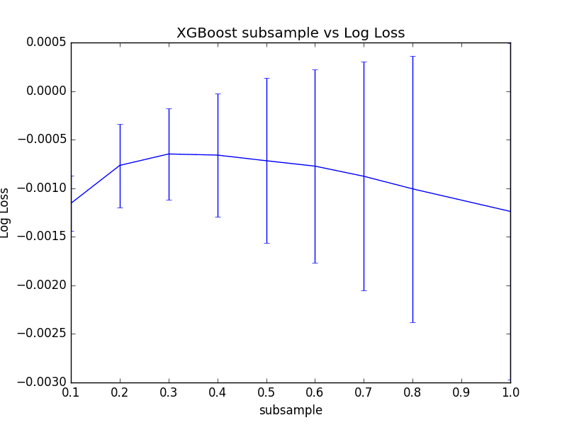
Plot of Tuning Row Sample Rate in XGBoost
We can see that indeed 30% has the best mean performance, but we can also see that as the ratio increased, the variance in performance grows quite markedly.
It is interesting to note that the mean performance of all subsample values outperforms the mean performance without subsampling (subsample=1.0).
Tuning Column Subsampling in XGBoost By Tree
We can also create a random sample of the features (or columns) to use prior to creating each decision tree in the boosted model.
In the XGBoost wrapper for scikit-learn, this is controlled by the colsample_bytree parameter.
The default value is 1.0 meaning that all columns are used in each decision tree. We can evaluate values for colsample_bytree between 0.1 and 1.0 incrementing by 0.1.
|
1 |
[0.1, 0.2, 0.3, 0.4, 0.5, 0.6, 0.7, 0.8, 1.0] |
The full code listing is provided below.
|
1 2 3 4 5 6 7 8 9 10 11 12 13 14 15 16 17 18 19 20 21 22 23 24 25 26 27 28 29 30 31 32 33 34 35 36 37 |
# XGBoost on Otto dataset, tune colsample_bytree from pandas import read_csv from xgboost import XGBClassifier from sklearn.model_selection import GridSearchCV from sklearn.model_selection import StratifiedKFold from sklearn.preprocessing import LabelEncoder import matplotlib matplotlib.use('Agg') from matplotlib import pyplot # load data data = read_csv('train.csv') dataset = data.values # split data into X and y X = dataset[:,0:94] y = dataset[:,94] # encode string class values as integers label_encoded_y = LabelEncoder().fit_transform(y) # grid search model = XGBClassifier() colsample_bytree = [0.1, 0.2, 0.3, 0.4, 0.5, 0.6, 0.7, 0.8, 1.0] param_grid = dict(colsample_bytree=colsample_bytree) kfold = StratifiedKFold(n_splits=10, shuffle=True, random_state=7) grid_search = GridSearchCV(model, param_grid, scoring="neg_log_loss", n_jobs=-1, cv=kfold) grid_result = grid_search.fit(X, label_encoded_y) # summarize results print("Best: %f using %s" % (grid_result.best_score_, grid_result.best_params_)) means = grid_result.cv_results_['mean_test_score'] stds = grid_result.cv_results_['std_test_score'] params = grid_result.cv_results_['params'] for mean, stdev, param in zip(means, stds, params): print("%f (%f) with: %r" % (mean, stdev, param)) # plot pyplot.errorbar(colsample_bytree, means, yerr=stds) pyplot.title("XGBoost colsample_bytree vs Log Loss") pyplot.xlabel('colsample_bytree') pyplot.ylabel('Log Loss') pyplot.savefig('colsample_bytree.png') |
Running this example prints the best configuration as well as the log loss for each tested configuration.
Note: Your results may vary given the stochastic nature of the algorithm or evaluation procedure, or differences in numerical precision. Consider running the example a few times and compare the average outcome.
We can see that the best performance for the model was colsample_bytree=1.0. This suggests that subsampling columns on this problem does not add value.
|
1 2 3 4 5 6 7 8 9 10 |
Best: -0.001239 using {'colsample_bytree': 1.0} -0.298955 (0.002177) with: {'colsample_bytree': 0.1} -0.092441 (0.000798) with: {'colsample_bytree': 0.2} -0.029993 (0.000459) with: {'colsample_bytree': 0.3} -0.010435 (0.000669) with: {'colsample_bytree': 0.4} -0.004176 (0.000916) with: {'colsample_bytree': 0.5} -0.002614 (0.001062) with: {'colsample_bytree': 0.6} -0.001694 (0.001221) with: {'colsample_bytree': 0.7} -0.001306 (0.001435) with: {'colsample_bytree': 0.8} -0.001239 (0.001730) with: {'colsample_bytree': 1.0} |
Plotting the results, we can see the performance of the model plateau (at least at this scale) with values between 0.5 to 1.0.
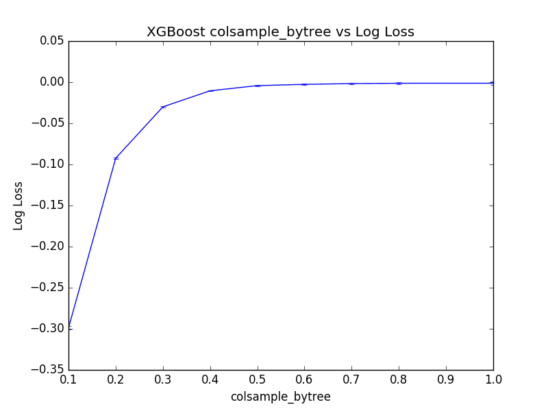
Plot of Tuning Per-Tree Column Sampling in XGBoost
Tuning Column Subsampling in XGBoost By Split
Rather than subsample the columns once for each tree, we can subsample them at each split in the decision tree. In principle, this is the approach used in random forest.
We can set the size of the sample of columns used at each split in the colsample_bylevel parameter in the XGBoost wrapper classes for scikit-learn.
As before, we will vary the ratio from 10% to the default of 100%.
The full code listing is provided below.
|
1 2 3 4 5 6 7 8 9 10 11 12 13 14 15 16 17 18 19 20 21 22 23 24 25 26 27 28 29 30 31 32 33 34 35 36 37 |
# XGBoost on Otto dataset, tune colsample_bylevel from pandas import read_csv from xgboost import XGBClassifier from sklearn.model_selection import GridSearchCV from sklearn.model_selection import StratifiedKFold from sklearn.preprocessing import LabelEncoder import matplotlib matplotlib.use('Agg') from matplotlib import pyplot # load data data = read_csv('train.csv') dataset = data.values # split data into X and y X = dataset[:,0:94] y = dataset[:,94] # encode string class values as integers label_encoded_y = LabelEncoder().fit_transform(y) # grid search model = XGBClassifier() colsample_bylevel = [0.1, 0.2, 0.3, 0.4, 0.5, 0.6, 0.7, 0.8, 1.0] param_grid = dict(colsample_bylevel=colsample_bylevel) kfold = StratifiedKFold(n_splits=10, shuffle=True, random_state=7) grid_search = GridSearchCV(model, param_grid, scoring="neg_log_loss", n_jobs=-1, cv=kfold) grid_result = grid_search.fit(X, label_encoded_y) # summarize results print("Best: %f using %s" % (grid_result.best_score_, grid_result.best_params_)) means = grid_result.cv_results_['mean_test_score'] stds = grid_result.cv_results_['std_test_score'] params = grid_result.cv_results_['params'] for mean, stdev, param in zip(means, stds, params): print("%f (%f) with: %r" % (mean, stdev, param)) # plot pyplot.errorbar(colsample_bylevel, means, yerr=stds) pyplot.title("XGBoost colsample_bylevel vs Log Loss") pyplot.xlabel('colsample_bylevel') pyplot.ylabel('Log Loss') pyplot.savefig('colsample_bylevel.png') |
Running this example prints the best configuration as well as the log loss for each tested configuration.
Note: Your results may vary given the stochastic nature of the algorithm or evaluation procedure, or differences in numerical precision. Consider running the example a few times and compare the average outcome.
We can see that the best results were achieved by setting colsample_bylevel to 70%, resulting in an (inverted) log loss of -0.001062, which is better than -0.001239 seen when setting the per-tree column sampling to 100%.
This suggest to not give up on column subsampling if per-tree results suggest using 100% of columns, and to instead try per-split column subsampling.
|
1 2 3 4 5 6 7 8 9 10 |
Best: -0.001062 using {'colsample_bylevel': 0.7} -0.159455 (0.007028) with: {'colsample_bylevel': 0.1} -0.034391 (0.003533) with: {'colsample_bylevel': 0.2} -0.007619 (0.000451) with: {'colsample_bylevel': 0.3} -0.002982 (0.000726) with: {'colsample_bylevel': 0.4} -0.001410 (0.000946) with: {'colsample_bylevel': 0.5} -0.001182 (0.001144) with: {'colsample_bylevel': 0.6} -0.001062 (0.001221) with: {'colsample_bylevel': 0.7} -0.001071 (0.001427) with: {'colsample_bylevel': 0.8} -0.001239 (0.001730) with: {'colsample_bylevel': 1.0} |
We can plot the performance of each colsample_bylevel variation. The results show relatively low variance and seemingly a plateau in performance after a value of 0.3 at this scale.
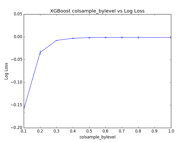
Plot of Tuning Per-Split Column Sampling in XGBoost
Summary
In this post you discovered stochastic gradient boosting with XGBoost in Python.
Specifically, you learned:
- About stochastic boosting and how you can subsample your training data to improve the generalization of your model
- How to tune row subsampling with XGBoost in Python and scikit-learn.
- How to tune column subsampling with XGBoost both per-tree and per-split.
Do you have any questions about stochastic gradient boosting or about this post? Ask your questions in the comments and I will do my best to answer.
Discover The Algorithm Winning Competitions!
Develop Your Own XGBoost Models in Minutes
...with just a few lines of Python
Discover how in my new Ebook:
XGBoost With Python
It covers self-study tutorials like:
Algorithm Fundamentals, Scaling, Hyperparameters, and much more...
Bring The Power of XGBoost To Your Own Projects
Skip the Academics. Just Results.


Hello Dr,
Good day sir. How can I plot the tuning of two variables simultaneously e.g gamma and learning_rate. Kind regards.
Consider saving the values to file for later plotting.
what is the accuracy of the model for different levels?
What do you mean by “different levels”?
Do you know how to obtain a probability distribution function “pdf” from gradient boosted trees. e.g. for Random Forests, we can use the distribution of predictions from each tree as a proxy for the pdf, and for AdaBoost one may weight the prediction from each tree by the weight of the tree, to get a “pdf”.
I’ve not found anything about this for gradient boosted trees…
Interesting idea. No sorry, you might have to write some custom code.
Another great article! Thanks. 🙂
You mentioned that Stochastic Gradient Boosting which implements column subsampling by split is very similar to how Random Forests operate. It seems that the difference is this:
For Random Forests, the split is based on selection of the column which results in the most homogenous split outcomes (a greedy algorithm).
For Stochastic Gradient Boosting implementing column subsampling by split, the split is based upon random selection of a column to be split.
Is this a correct understanding of the distinction between these two methods?
Thanks!
I believe so.
Hi Jason,
Do you have a plan to write another book or a tutorial about using XGBoost in time series problems/predictions?
Great suggestion. Not at this stage, but I like the idea!
It will be awesome.
Thank you so much.
Man your work is awesome, You deserve a medal. My M.L. skills have greatly improved thanks to you.
Question : What do I stand to loose if I tune multiple parameters at the same time in the same cell.
E.g Tuning subsample, colsample_bytree & colsample_bylevel on the same cell using the same method of selecting parameter samples to be used, saving them in a dictionary then parsing KFold and GridSearchCV
Thanks Ted! I’m glad the posts help.
You can tune multiple parameters at the same time – it’s a great idea, it can just be slow – computationally expensive to run.
Very nice article. My question is, why did you not “keep” the optimal parameters found (row subsampling of 0.3) for the next steps?
In the end, we want to find the best combination of the subsampling parameters for rows by tree, columns by tree, and columns by level. Testing everything at once in a GridSearch is very time-consuming. However, if you do it iteratively, wouldn’t it make sense to keep the previously found optimal parameter while testing for other kinds of subsampling?
Yes, but in this tutorial we are demonstrating the effect of the hyperparameters, not trying to best solve the prediction problem.
Hi Jason,
I have a question. when tuning the multiple hyperparameters to try to best solve the prediction problem, tuning all the hyperparameters together will be accurate but slow. If every time tuning subset of hyperparameters can get the best solution?
Thank you in advance!
Yes, all at once is slow, one by one might miss a combination. It is a trade-off.
Hi Jason,
What’s the difference of the auc score between the training set and validation set or test set will be better? I mean that the model will predict other samples with high score. I trained a model that the auc of training set is 0.87, the auc of validation set is 0.81, and the auc of test set is 0.83. but the auc for predicting other set is only 0.6. Could you give me some advaices. Thank you in advance.
If you are performing model selection, then you only need to consider the performance of the model on the out of sample (test) datasets.
Thank you for your reply. The performance for predicting the test datasets when building model is well. But using the model to predict the practical dataset proved practically bad! How could I do?
Perhaps confirm that your test set is representative of the problem?
Perhaps try repeated k-fold cross-validation to estimate performance?
Perhaps the new data is very different to the data you used?
Perhaps ensure that you’re preparing the new data in an identical manner to the training data?