Stochastic Hill climbing is an optimization algorithm.
It makes use of randomness as part of the search process. This makes the algorithm appropriate for nonlinear objective functions where other local search algorithms do not operate well.
It is also a local search algorithm, meaning that it modifies a single solution and searches the relatively local area of the search space until the local optima is located. This means that it is appropriate on unimodal optimization problems or for use after the application of a global optimization algorithm.
In this tutorial, you will discover the hill climbing optimization algorithm for function optimization
After completing this tutorial, you will know:
Hill climbing is a stochastic local search algorithm for function optimization.
How to implement the hill climbing algorithm from scratch in Python.
How to apply the hill climbing algorithm and inspect the results of the algorithm.
Kick-start your project with my new book Optimization for Machine Learning, including step-by-step tutorials and the Python source code files for all examples.
Let’s get started.
Stochastic Hill Climbing in Python from Scratch Photo by John, some rights reserved.
Tutorial Overview
This tutorial is divided into three parts; they are:
Hill Climbing Algorithm
Hill Climbing Algorithm Implementation
Example of Applying the Hill Climbing Algorithm
Hill Climbing Algorithm
The stochastic hill climbing algorithm is a stochastic local search optimization algorithm.
It takes an initial point as input and a step size, where the step size is a distance within the search space.
The algorithm takes the initial point as the current best candidate solution and generates a new point within the step size distance of the provided point. The generated point is evaluated, and if it is equal or better than the current point, it is taken as the current point.
The generation of the new point uses randomness, often referred to as Stochastic Hill Climbing. This means that the algorithm can skip over bumpy, noisy, discontinuous, or deceptive regions of the response surface as part of the search.
Stochastic hill climbing chooses at random from among the uphill moves; the probability of selection can vary with the steepness of the uphill move.
It is important that different points with equal evaluation are accepted as it allows the algorithm to continue to explore the search space, such as across flat regions of the response surface. It may also be helpful to put a limit on these so-called “sideways” moves to avoid an infinite loop.
If we always allow sideways moves when there are no uphill moves, an infinite loop will occur whenever the algorithm reaches a flat local maximum that is not a shoulder. One common solution is to put a limit on the number of consecutive sideways moves allowed. For example, we could allow up to, say, 100 consecutive sideways moves
This process continues until a stop condition is met, such as a maximum number of function evaluations or no improvement within a given number of function evaluations.
The algorithm takes its name from the fact that it will (stochastically) climb the hill of the response surface to the local optima. This does not mean it can only be used for maximizing objective functions; it is just a name. In fact, typically, we minimize functions instead of maximize them.
The hill-climbing search algorithm (steepest-ascent version) […] is simply a loop that continually moves in the direction of increasing value—that is, uphill. It terminates when it reaches a “peak” where no neighbor has a higher value.
The step size must be large enough to allow better nearby points in the search space to be located, but not so large that the search jumps over out of the region that contains the local optima.
Want to Get Started With Optimization Algorithms?
Take my free 7-day email crash course now (with sample code).
Click to sign-up and also get a free PDF Ebook version of the course.
Hill Climbing Algorithm Implementation
At the time of writing, the SciPy library does not provide an implementation of stochastic hill climbing.
Nevertheless, we can implement it ourselves.
First, we must define our objective function and the bounds on each input variable to the objective function. The objective function is just a Python function we will name objective(). The bounds will be a 2D array with one dimension for each input variable that defines the minimum and maximum for the variable.
For example, a one-dimensional objective function and bounds would be defined as follows:
1
2
3
4
5
6
# objective function
def objective(x):
return0
# define range for input
bounds=asarray([[-5.0,5.0]])
Next, we can generate our initial solution as a random point within the bounds of the problem, then evaluate it using the objective function.
Now we can loop over a predefined number of iterations of the algorithm defined as “n_iterations“, such as 100 or 1,000.
1
2
3
4
...
# run the hill climb
foriinrange(n_iterations):
...
The first step of the algorithm iteration is to take a step.
This requires a predefined “step_size” parameter, which is relative to the bounds of the search space. We will take a random step with a Gaussian distribution where the mean is our current point and the standard deviation is defined by the “step_size“. That means that about 99 percent of the steps taken will be within (3 * step_size) of the current point.
1
2
3
...
# take a step
candidate=solution+randn(len(bounds))*step_size
We don’t have to take steps in this way. You may wish to use a uniform distribution between 0 and the step size. For example:
1
2
3
...
# take a step
candidate=solution+rand(len(bounds))*step_size
Next we need to evaluate the new candidate solution with the objective function.
1
2
3
...
# evaluate candidate point
candidte_eval=objective(candidate)
We then need to check if the evaluation of this new point is as good as or better than the current best point, and if it is, replace our current best point with this new point.
We can implement this hill climbing algorithm as a reusable function that takes the name of the objective function, the bounds of each input variable, the total iterations and steps as arguments, and returns the best solution found and its evaluation.
Now that we know how to implement the hill climbing algorithm in Python, let’s look at how we might use it to optimize an objective function.
Example of Applying the Hill Climbing Algorithm
In this section, we will apply the hill climbing optimization algorithm to an objective function.
First, let’s define our objective function.
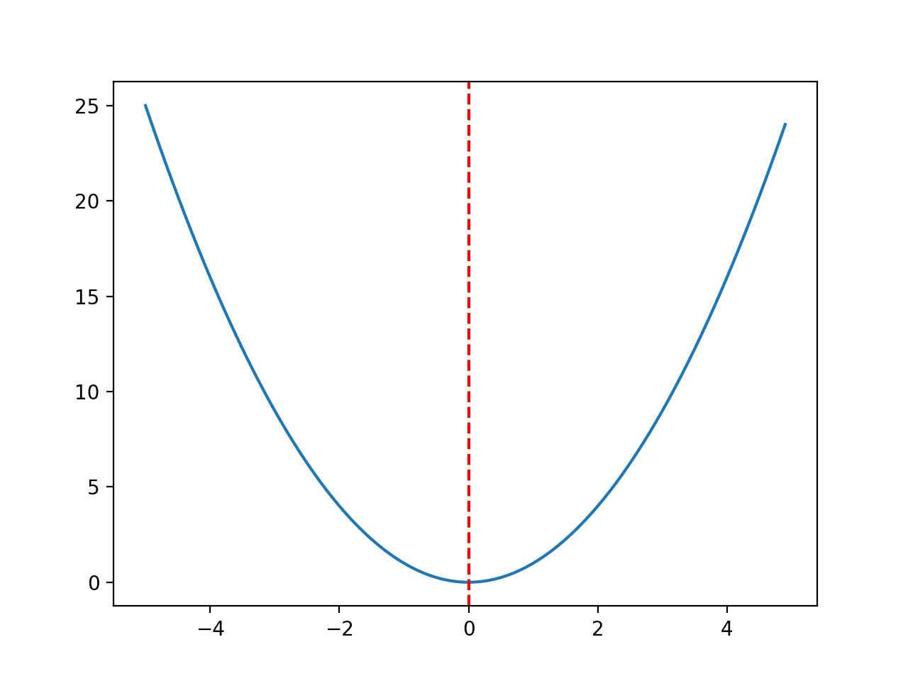
We will use a simple one-dimensional x^2 objective function with the bounds [-5, 5].
The example below defines the function, then creates a line plot of the response surface of the function for a grid of input values and marks the optima at f(0.0) = 0.0 with a red line.
1
2
3
4
5
6
7
8
9
10
11
12
13
14
15
16
17
18
19
20
21
22
# convex unimodal optimization function
from numpy import arange
from matplotlib import pyplot
# objective function
def objective(x):
returnx[0]**2.0
# define range for input
r_min,r_max=-5.0,5.0
# sample input range uniformly at 0.1 increments
inputs=arange(r_min,r_max,0.1)
# compute targets
results=[objective([x])forxininputs]
# create a line plot of input vs result
pyplot.plot(inputs,results)
# define optimal input value
x_optima=0.0
# draw a vertical line at the optimal input
pyplot.axvline(x=x_optima,ls='--',color='red')
# show the plot
pyplot.show()
Running the example creates a line plot of the objective function and clearly marks the function optima.
Line Plot of Objective Function With Optima Marked with a Dashed Red Line
Next, we can apply the hill climbing algorithm to the objective function.
First, we will seed the pseudorandom number generator. This is not required in general, but in this case, I want to ensure we get the same results (same sequence of random numbers) each time we run the algorithm so we can plot the results later.
1
2
3
...
# seed the pseudorandom number generator
seed(5)
Next, we can define the configuration of the search.
In this case, we will search for 1,000 iterations of the algorithm and use a step size of 0.1. Given that we are using a Gaussian function for generating the step, this means that about 99 percent of all steps taken will be within a distance of (0.1 * 3) of a given point, e.g. three standard deviations.
1
2
3
4
...
n_iterations=1000
# define the maximum step size
step_size=0.1
Next, we can perform the search and report the results.
Running the example reports the progress of the search, including the iteration number, the input to the function, and the response from the objective function each time an improvement was detected.
At the end of the search, the best solution is found and its evaluation is reported.
In this case we can see about 36 improvements over the 1,000 iterations of the algorithm and a solution that is very close to the optimal input of 0.0 that evaluates to f(0.0) = 0.0.
1
2
3
4
5
6
7
8
9
10
11
12
13
14
15
16
17
18
19
20
21
22
23
24
25
26
27
28
29
30
31
32
33
34
35
36
37
38
>1 f([-2.74290923]) = 7.52355
>3 f([-2.65873147]) = 7.06885
>4 f([-2.52197291]) = 6.36035
>5 f([-2.46450214]) = 6.07377
>7 f([-2.44740961]) = 5.98981
>9 f([-2.28364676]) = 5.21504
>12 f([-2.19245939]) = 4.80688
>14 f([-2.01001538]) = 4.04016
>15 f([-1.86425287]) = 3.47544
>22 f([-1.79913002]) = 3.23687
>24 f([-1.57525573]) = 2.48143
>25 f([-1.55047719]) = 2.40398
>26 f([-1.51783757]) = 2.30383
>27 f([-1.49118756]) = 2.22364
>28 f([-1.45344116]) = 2.11249
>30 f([-1.33055275]) = 1.77037
>32 f([-1.17805016]) = 1.38780
>33 f([-1.15189314]) = 1.32686
>36 f([-1.03852644]) = 1.07854
>37 f([-0.99135322]) = 0.98278
>38 f([-0.79448984]) = 0.63121
>39 f([-0.69837955]) = 0.48773
>42 f([-0.69317313]) = 0.48049
>46 f([-0.61801423]) = 0.38194
>48 f([-0.48799625]) = 0.23814
>50 f([-0.22149135]) = 0.04906
>54 f([-0.20017144]) = 0.04007
>57 f([-0.15994446]) = 0.02558
>60 f([-0.15492485]) = 0.02400
>61 f([-0.03572481]) = 0.00128
>64 f([-0.03051261]) = 0.00093
>66 f([-0.0074283]) = 0.00006
>78 f([-0.00202357]) = 0.00000
>119 f([0.00128373]) = 0.00000
>120 f([-0.00040911]) = 0.00000
>314 f([-0.00017051]) = 0.00000
Done!
f([-0.00017051]) = 0.000000
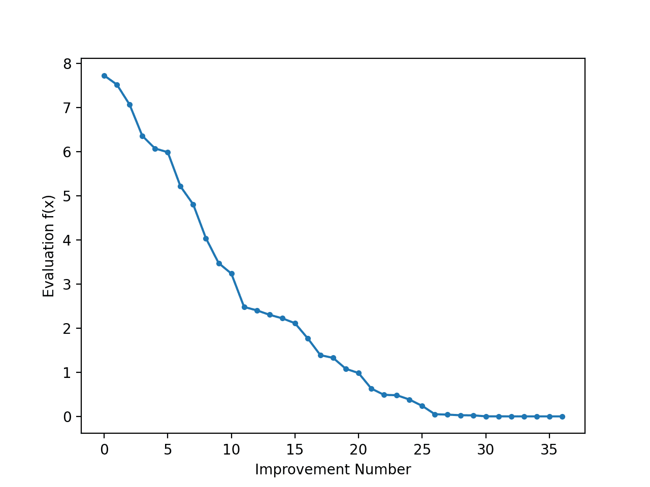
It can be interesting to review the progress of the search as a line plot that shows the change in the evaluation of the best solution each time there is an improvement.
We can update the hillclimbing() to keep track of the objective function evaluations each time there is an improvement and return this list of scores.
We can then create a line plot of these scores to see the relative change in objective function for each improvement found during the search.
1
2
3
4
5
6
...
# line plot of best scores
pyplot.plot(scores,'.-')
pyplot.xlabel('Improvement Number')
pyplot.ylabel('Evaluation f(x)')
pyplot.show()
Tying this together, the complete example of performing the search and plotting the objective function scores of the improved solutions during the search is listed below.
1
2
3
4
5
6
7
8
9
10
11
12
13
14
15
16
17
18
19
20
21
22
23
24
25
26
27
28
29
30
31
32
33
34
35
36
37
38
39
40
41
42
43
44
45
46
47
48
49
50
51
52
# hill climbing search of a one-dimensional objective function
Running the example performs the search and reports the results as before.
A line plot is created showing the objective function evaluation for each improvement during the hill climbing search. We can see about 36 changes to the objective function evaluation during the search, with large changes initially and very small to imperceptible changes towards the end of the search as the algorithm converged on the optima.
Line Plot of Objective Function Evaluation for Each Improvement During the Hill Climbing Search
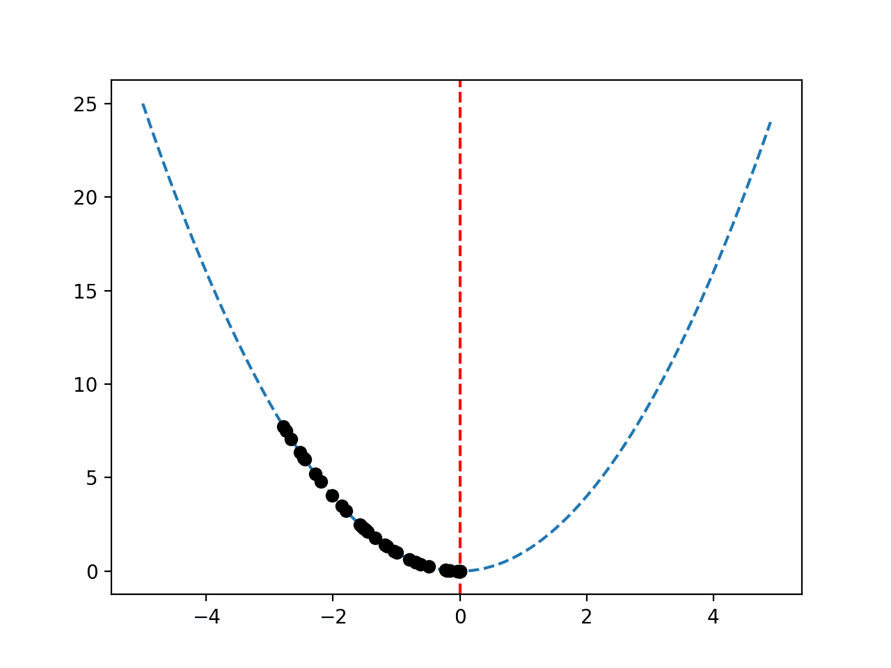
Given that the objective function is one-dimensional, it is straightforward to plot the response surface as we did above.
It can be interesting to review the progress of the search by plotting the best candidate solutions found during the search as points in the response surface. We would expect a sequence of points running down the response surface to the optima.
This can be achieved by first updating the hillclimbing() function to keep track of each best candidate solution as it is located during the search, then return a list of best solutions.
Tying this together, the complete example of plotting the sequence of improved solutions on the response surface of the objective function is listed below.
1
2
3
4
5
6
7
8
9
10
11
12
13
14
15
16
17
18
19
20
21
22
23
24
25
26
27
28
29
30
31
32
33
34
35
36
37
38
39
40
41
42
43
44
45
46
47
48
49
50
51
52
53
54
55
56
57
# hill climbing search of a one-dimensional objective function
Running the example performs the hill climbing search and reports the results as before.
A plot of the response surface is created as before showing the familiar bowl shape of the function with a vertical red line marking the optima of the function.
The sequence of best solutions found during the search is shown as black dots running down the bowl shape to the optima.
Response Surface of Objective Function With Sequence of Best Solutions Plotted as Black Dots
Further Reading
This section provides more resources on the topic if you are looking to go deeper.
It provides self-study tutorials with full working code on: Gradient Descent, Genetic Algorithms, Hill Climbing, Curve Fitting, RMSProp, Adam,
and much more...
Bring Modern Optimization Algorithms to Your Machine Learning Projects
The experiment approach. If we had ordinary math functions with 784 input variables we could make experiments where you know the global minimum in advance. Then as the experiment sample 100 points as input to a machine learning function y = model(X). Train on yt,Xt as the global minimum. Loss = 0. Could be useful to train hyper params in general?
Questions please:
(1) Could a hill climbing algorithm determine a maxima and minima of the equation?
(2) I know Newton’s method for solving minima (say). It is an iterative algorithm of the form
1
x(n+1)=x(n)-f(x(n))/f'(x(n))
Iteration stops when the difference x(n) – f(x(n))/f'(x(n)) is < determined value.
In other words, what does the hill climbing algorithm have over the Newton Method?
Yes to the first part, not quite for the second part.
There are tens (hundreds) of alternative algorithms that can be used for multimodal optimization problems, including repeated application of hill climbing (e.g. hill climbing with multiple restarts). Grid search might be one of the least efficient approaches to searching a domain, but great if you have a small domain or tons of compute/time.


The experiment approach. If we had ordinary math functions with 784 input variables we could make experiments where you know the global minimum in advance. Then as the experiment sample 100 points as input to a machine learning function y = model(X). Train on yt,Xt as the global minimum. Loss = 0. Could be useful to train hyper params in general?
Sure.
Dear Dr Jason,
What if you have a function with say a number of minima and maxima as in a calculus problem. Example of graph with minima and maxima at https://scientificsentence.net/Equations/CalculusII/extrema.jpg .
Questions please:
(1) Could a hill climbing algorithm determine a maxima and minima of the equation?
(2) I know Newton’s method for solving minima (say). It is an iterative algorithm of the form
Iteration stops when the difference x(n) – f(x(n))/f'(x(n)) is < determined value.
In other words, what does the hill climbing algorithm have over the Newton Method?
Thank you,
Anthony of Sydney
Hill climbing is typically appropriate for a unimodal (single optima) problems.
You could apply it many times to sniff out the optima, but you may as well grid search the domain.
Hill climbing does not require a first or second order gradient, it does not require the objective function to be differentiable.
Dear Dr Jason,
The takeaway – hill climbing is unimodal and does not require derivatives i.e. calculus. For multiple minima and maxima use gridsearch.
Thank you, grateful for this.
Anthony of Sydney
Yes to the first part, not quite for the second part.
There are tens (hundreds) of alternative algorithms that can be used for multimodal optimization problems, including repeated application of hill climbing (e.g. hill climbing with multiple restarts). Grid search might be one of the least efficient approaches to searching a domain, but great if you have a small domain or tons of compute/time.
Dear Dr Jason,
Thank you,
Anthony of Sydney