Ensembles are a machine learning method that combine the predictions from multiple models in an effort to achieve better predictive performance.
There are many different types of ensembles, although all approaches have two key properties: they require that the contributing models are different so that they make different errors and they combine the predictions in an attempt to harness what each different model does well.
Nevertheless, it is not clear how ensembles manage to achieve this, especially in the context of classification and regression type predictive modeling problems. It is important to develop an intuition for what exactly ensembles are doing when they combine predictions as it will help choose and configure appropriate models on predictive modeling projects.
In this post, you will discover the intuition behind how ensemble learning methods work.
After reading this post, you will know:
Ensemble learning methods work by combining the mapping functions learned by contributing members.
Ensembles for classification are best understood by the combination of decision boundaries of members.
Ensembles for regression are best understood by the combination of hyperplanes of members.
Kick-start your project with my new book Ensemble Learning Algorithms With Python, including step-by-step tutorials and the Python source code files for all examples.
Let’s get started.
Develop an Intuition for How Ensemble Learning Works Photo by Marco Verch, some rights reserved.
Tutorial Overview
This tutorial is divided into three parts; they are:
How Do Ensembles Work
Intuition for Classification Ensembles
Intuition for Regression Ensembles
How Do Ensembles Work
Ensemble learning refers to combining the predictions from two or more models.
The goal of using ensemble methods is to improve the skill of predictions over that of any of the contributing members.
This objective is straightforward but it is less clear how exactly ensemble methods are able to achieve this.
It is important to develop an intuition for how ensemble techniques work as it will help you both choose and configure specific ensemble methods for a prediction task and interpret their results to come up with alternative ways to further improve performance.
Consider a simple ensemble that trains two models on slightly different samples of the training dataset and averages their predictions.
Each of the member models can be used in a standalone manner to make predictions, although the hope is that averaging their predictions improves their performance. This can only be the case if each model makes different predictions.
Different predictions mean that in some cases, model 1 will make few errors and model 2 will make more errors, and the reverse for other cases. Averaging their predictions seeks to reduce these errors across the predictions made by both models.
In turn, for the models to make different predictions, they must make different assumptions about the prediction problem. More specifically, they must learn a different mapping function from inputs to outputs. We can achieve this in the simple case by training each model on a different sample of the training dataset, but there are many additional ways that we could achieve this difference; training different model types is one.
These elements are how and ensemble methods work in the general sense, namely:
Members learn different mapping functions for the same problem. This is to ensure that models make different prediction errors.
Predictions made by members are combined in some way. This is to ensure that the differences in prediction errors are exploited.
We don’t simply smooth out the prediction errors, although we can; instead, we smooth out the mapping function learned by the contributing members.
The improved mapping function allows better predictions to be made.
This is a deeper point and it is important that we understand it. Let’s take a closer look at what it means for both classification and regression tasks.
Want to Get Started With Ensemble Learning?
Take my free 7-day email crash course now (with sample code).
Click to sign-up and also get a free PDF Ebook version of the course.
A model may predict a crisp class label, e.g. a categorical variable, or the probabilities for all possible categorical outcomes.
In the simple case, the crisp class labels predicted by ensemble members can be combined by voting, e.g. the statistical mode or label with the most votes determines the ensemble outcome. Class probabilities predicted by ensemble members can be summed and normalized.
Functionally, some process like this is occurring in an ensemble for a classification task, but the effect is on the mapping function from input examples to class labels or probabilities. Let’s stick with labels for now.
The most common way to think about the mapping function for classification is by using a plot where the input data represents a point in an n-dimensional space defined by the extent of the input variables, called the feature space. For example, if we had two input features, x and y, both in the range zero to one, then the input space would be two-dimensional plane and each example in the dataset would be a point on that plane. Each point can then be assigned a color or shape based on the class label.
A model that learns how to classify points in effect draws lines in the feature space to separate examples. We can sample points in the feature space in a grid and get a map of how the model thinks the feature space should be by each class label.
The separation of examples in the feature space by the model is called the decision boundary and a plot of the grid or map of how the model classifies points in the feature space is called a decision boundary plot.
Now consider an ensemble where each model has a different mapping of inputs to outputs. In effect, each model has a different decision boundary or different idea of how to split up in the feature space by class label. Each model will draw the lines differently and make different errors.
When we combine the predictions from these multiple different models, we are in effect averaging the decision boundaries. We are defining a new decision boundary that attempts to learn from all the different views on the feature space learned by contributing members.
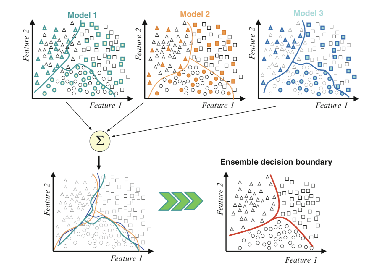
The figure below taken from Page 1 of “Ensemble Machine Learning” provides a useful depiction of this.
Example of Combining Decision Boundaries Using an Ensemble Taken from Ensemble Machine Learning, 2012.
We can see the contributing members along the top, each with different decision boundaries in the feature space. Then the bottom-left draws all of the decision boundaries on the same plot showing how they differ and make different errors.
Finally, we can combine these boundaries to create a new generalized decision boundary in the bottom-right that better captures the true but unknown division of the feature space, resulting in better predictive performance.
Intuition for Regression Ensembles
Regression predictive modeling refers to problems where a numerical value must be predicted from examples of input.
In the simple case, the numeric predictions made by ensemble members can be combined using statistical measures like the mean, although more complex combinations can be used.
Like classification, the effect of the ensemble is that the mapping functions of each contributing member are averaged or combined.
The most common way to think about the mapping function for regression is by using a line plot where the output variable is another dimension added to the input feature space. The relationship of the feature space and the target variable dimension can then be summarized as a hyperplane, e.g. a line in many dimensions.
This is mind-bending, so let’s consider the simplest case where we have one numerical input and one numerical output. Consider a plane or graph where the x-axis represents the input feature and the y-axis represents the target variable. We can plot each example in the dataset as a point on this plot.
A model that learns the mapping from input to outputs in effect learns a hyperplane that connects the points in the feature space to the target variable. We can sample a grid of points in the input feature space to devise values for the target variable and draw a line to connect them to represent this hyperplane.
In our two-dimensional case, this is a line that passes through the points on the plot. Any point where the line does not pass through the plot represents a prediction error and the distance from the line to the point is the magnitude of the error.
Now consider an ensemble where each model has a different mapping of inputs to outputs. In effect, each model has a different hyperplane connecting the feature space to the target. Each model will draw different lines and make different errors with different magnitudes.
When we combine the predictions from these multiple different models we are, in effect, averaging the hyperplanes. We are defining a new hyperplane that attempts to learn from all the different features on how to map inputs to outputs.
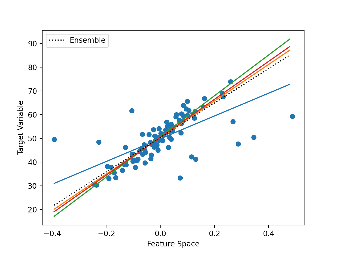
The figure below gives an example of a one-dimensional input feature space and a target space with different learned hyperplane mappings.
Example of Combining Hyperplanes Using an Ensemble
We can see the dots representing points from the training dataset. We can also see a number of different straight lines through the data. The models do not have to learn straight lines, but in this case, they have.
Finally, we can see a dashed black line that shows the ensemble average of all of the models, resulting in lower prediction error.
Further Reading
This section provides more resources on the topic if you are looking to go deeper.
Dear Dr Jason,
Thank you for whetting the appetite especially with the 2nd last photo “Example of Combining Decision Boundaries Using an Ensemble Taken from Ensemble Machine Learning, 2012”
Have you done or could you do an example of Combinng Decision Boundaries Using an Ensemble on the “Iris Data Set”. Note I have seen plots of “Sepal Lengths” vs Sepal Widths” for the four different species iris.
It would be a great example of predicting which species the flower belongs according to .sepal width and sepal length.
Dear Dr Jason,
Do you have any python code in your site that shows the those lines which are the boundaries between ‘sepal length’ vs ‘sepal width’ for a particular iris species setosa, virginica and versicolor AND ‘petal length’ vs ‘petal width’ for a particular iris species setosa, virginica and versicolor – something similar to the diagram at https://i.stack.imgur.com/YijL7.png
Need clarity please especially the model and where there is data from one species in the boundary of another species.
Dear Dr Jason,
Thank you for that.
In addition, knowing the name of the technique, the key words are: plotting, decision surface.
I found more sites. Basically it is the same technique used in the aforementioned site “plot-a-decision-surface-for-machine-learning”.
The key is learning how to restructure the ‘data’ based on the min and max of each feature NOT on the actual data. From the aranged, meshed, flattened data, we make a mesh grid and predict on the mesh grid.
There is more detail, but the key is to learn how to restructure data.


Dear Dr Jason,
Thank you for whetting the appetite especially with the 2nd last photo “Example of Combining Decision Boundaries Using an Ensemble Taken from Ensemble Machine Learning, 2012”
Have you done or could you do an example of Combinng Decision Boundaries Using an Ensemble on the “Iris Data Set”. Note I have seen plots of “Sepal Lengths” vs Sepal Widths” for the four different species iris.
It would be a great example of predicting which species the flower belongs according to .sepal width and sepal length.
Thank you,
Anthony of Sydney
You can use any ensemble you like to combine the decision boundaries of the submodels.
E.g. plot the decision boundary of each sub model then use a voting ensemble and plot the boundary of the ensemble to compare.
Dear Dr Jason,
Do you have any python code in your site that shows the those lines which are the boundaries between ‘sepal length’ vs ‘sepal width’ for a particular iris species setosa, virginica and versicolor AND ‘petal length’ vs ‘petal width’ for a particular iris species setosa, virginica and versicolor – something similar to the diagram at https://i.stack.imgur.com/YijL7.png
Need clarity please especially the model and where there is data from one species in the boundary of another species.
Thank you,
No, but this tutorial will show you how to draw such lines for a given dataset:
https://machinelearningmastery.com/plot-a-decision-surface-for-machine-learning/
Dear Dr Jason,
Thank you for that.
In addition, knowing the name of the technique, the key words are: plotting, decision surface.
I found more sites. Basically it is the same technique used in the aforementioned site “plot-a-decision-surface-for-machine-learning”.
The key is learning how to restructure the ‘data’ based on the min and max of each feature NOT on the actual data. From the aranged, meshed, flattened data, we make a mesh grid and predict on the mesh grid.
There is more detail, but the key is to learn how to restructure data.
Thank you,
Anthony of Sydney
Thanks for such a lucid explanation on ensemble learning
You’re welcome.