Particle swarm optimization (PSO) is one of the bio-inspired algorithms and it is a simple one to search for an optimal solution in the solution space. It is different from other optimization algorithms in such a way that only the objective function is needed and it is not dependent on the gradient or any differential form of the objective. It also has very few hyperparameters.
In this tutorial, you will learn the rationale of PSO and its algorithm with an example. After competing this tutorial, you will know:
- What is a particle swarm and their behavior under the PSO algorithm
- What kind of optimization problems can be solved by PSO
- How to solve a problem using particle swarm optimization
- What are the variations of the PSO algorithm
Kick-start your project with my new book Optimization for Machine Learning, including step-by-step tutorials and the Python source code files for all examples.
Let’s get started.Particle Swarms
Particle Swarm Optimization was proposed by Kennedy and Eberhart in 1995. As mentioned in the original paper, sociobiologists believe a school of fish or a flock of birds that moves in a group “can profit from the experience of all other members”. In other words, while a bird flying and searching randomly for food, for instance, all birds in the flock can share their discovery and help the entire flock get the best hunt.

Particle Swarm Optimizsation.
Photo by Don DeBold, some rights reserved.
While we can simulate the movement of a flock of birds, we can also imagine each bird is to help us find the optimal solution in a high-dimensional solution space and the best solution found by the flock is the best solution in the space. This is a heuristic solution because we can never prove the real global optimal solution can be found and it is usually not. However, we often find that the solution found by PSO is quite close to the global optimal.
Example Optimization Problem
PSO is best used to find the maximum or minimum of a function defined on a multidimensional vector space. Assume we have a function $f(X)$ that produces a real value from a vector parameter $X$ (such as coordinate $(x,y)$ in a plane) and $X$ can take on virtually any value in the space (for example, $f(X)$ is the altitude and we can find one for any point on the plane), then we can apply PSO. The PSO algorithm will return the parameter $X$ it found that produces the minimum $f(X)$.
Let’s start with the following function
$$
f(x,y) = (x-3.14)^2 + (y-2.72)^2 + \sin(3x+1.41) + \sin(4y-1.73)
$$
Plot of f(x,y)
As we can see from the plot above, this function looks like a curved egg carton. It is not a convex function and therefore it is hard to find its minimum because a local minimum found is not necessarily the global minimum.
So how can we find the minimum point in this function? For sure, we can resort to exhaustive search: If we check the value of $f(x,y)$ for every point on the plane, we can find the minimum point. Or we can just randomly find some sample points on the plane and see which one gives the lowest value on $f(x,y)$ if we think it is too expensive to search every point. However, we also note from the shape of $f(x,y)$ that if we have found a point with a smaller value of $f(x,y)$, it is easier to find an even smaller value around its proximity.
This is how a particle swarm optimization does. Similar to the flock of birds looking for food, we start with a number of random points on the plane (call them particles) and let them look for the minimum point in random directions. At each step, every particle should search around the minimum point it ever found as well as around the minimum point found by the entire swarm of particles. After certain iterations, we consider the minimum point of the function as the minimum point ever explored by this swarm of particles.
Want to Get Started With Optimization Algorithms?
Take my free 7-day email crash course now (with sample code).
Click to sign-up and also get a free PDF Ebook version of the course.
Algorithm Details
Assume we have $P$ particles and we denote the position of particle $i$ at iteration $t$ as $X^i(t)$, which in the example of above, we have it as a coordinate $X^i(t) = (x^i(t), y^i(t)).$ Besides the position, we also have a velocity for each particle, denoted as $V^i(t)=(v_x^i(t), v_y^i(t))$. At the next iteration, the position of each particle would be updated as
$$
X^i(t+1) = X^i(t)+V^i(t+1)
$$
or, equivalently,
$$
\begin{aligned}
x^i(t+1) &= x^i(t) + v_x^i(t+1) \\
y^i(t+1) &= y^i(t) + v_y^i(t+1)
\end{aligned}
$$
and at the same time, the velocities are also updated by the rule
$$
V^i(t+1) =
w V^i(t) + c_1r_1(pbest^i – X^i(t)) + c_2r_2(gbest – X^i(t))
$$
where $r_1$ and $r_2$ are random numbers between 0 and 1, constants $w$, $c_1$, and $c_2$ are parameters to the PSO algorithm, and $pbest^i$ is the position that gives the best $f(X)$ value ever explored by particle $i$ and $gbest$ is that explored by all the particles in the swarm.
Note that $pbest^i$ and $X^i(t)$ are two position vectors and the difference $pbest^i – X^i(t)$ is a vector subtraction. Adding this subtraction to the original velocity $V^i(t)$ is to bring the particle back to the position $pbest^i$. Similar are for the difference $gbest – X^i(t)$.

Vector subtraction.
Diagram by Benjamin D. Esham, public domain.
We call the parameter $w$ the inertia weight constant. It is between 0 and 1 and determines how much should the particle keep on with its previous velocity (i.e., speed and direction of the search). The parameters $c_1$ and $c_2$ are called the cognitive and the social coefficients respectively. They controls how much weight should be given between refining the search result of the particle itself and recognizing the search result of the swarm. We can consider these parameters controls the trade off between exploration and exploitation.
The positions $pbest^i$ and $gbest$ are updated in each iteration to reflect the best position ever found thus far.
One interesting property of this algorithm that distinguishs it from other optimization algorithms is that it does not depend on the gradient of the objective function. In gradient descent, for example, we look for the minimum of a function $f(X)$ by moving $X$ to the direction of $-\nabla f(X)$ as it is where the function going down the fastest. For any particle at the position $X$ at the moment, how it moves does not depend on which direction is the “down hill” but only on where are $pbest$ and $gbest$. This makes PSO particularly suitable if differentiating $f(X)$ is difficult.
Another property of PSO is that it can be parallelized easily. As we are manipulating multiple particles to find the optimal solution, each particles can be updated in parallel and we only need to collect the updated value of $gbest$ once per iteration. This makes map-reduce architecture a perfect candidate to implement PSO.
Implementation
Here we show how we can implement PSO to find the optimal solution.
For the same function as we showed above, we can first define it as a Python function and show it in a contour plot:
|
1 2 3 4 5 6 7 8 9 10 11 12 13 14 15 16 17 18 19 |
import numpy as np import matplotlib.pyplot as plt def f(x,y): "Objective function" return (x-3.14)**2 + (y-2.72)**2 + np.sin(3*x+1.41) + np.sin(4*y-1.73) # Contour plot: With the global minimum showed as "X" on the plot x, y = np.array(np.meshgrid(np.linspace(0,5,100), np.linspace(0,5,100))) z = f(x, y) x_min = x.ravel()[z.argmin()] y_min = y.ravel()[z.argmin()] plt.figure(figsize=(8,6)) plt.imshow(z, extent=[0, 5, 0, 5], origin='lower', cmap='viridis', alpha=0.5) plt.colorbar() plt.plot([x_min], [y_min], marker='x', markersize=5, color="white") contours = plt.contour(x, y, z, 10, colors='black', alpha=0.4) plt.clabel(contours, inline=True, fontsize=8, fmt="%.0f") plt.show() |
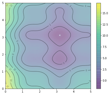
Contour plot of f(x,y)
Here we plotted the function $f(x,y)$ in the region of $0\le x,y\le 5$. We can create 20 particles at random locations in this region, together with random velocities sampled over a normal distribution with mean 0 and standard deviation 0.1, as follows:
|
1 2 3 |
n_particles = 20 X = np.random.rand(2, n_particles) * 5 V = np.random.randn(2, n_particles) * 0.1 |
which we can show their position on the same contour plot:
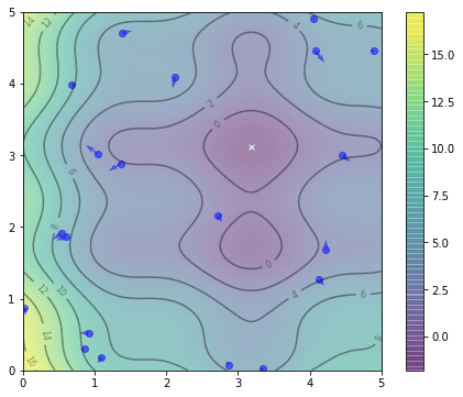
Initial position of particles
From this, we can already find the $gbest$ as the best position ever found by all the particles. Since the particles did not explore at all, their current position is their $pbest^i$ as well:
|
1 2 3 4 |
pbest = X pbest_obj = f(X[0], X[1]) gbest = pbest[:, pbest_obj.argmin()] gbest_obj = pbest_obj.min() |
The vector pbest_obj is the best value of the objective function found by each particle. Similarly, gbest_obj is the best scalar value of the objective function ever found by the swarm. We are using min() and argmin() functions here because we set it as a minimization problem. The position of gbest is marked as a star below
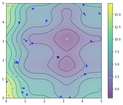
Position of gbest is marked as a star
Let’s set $c_1=c_2=0.1$ and $w=0.8$. Then we can update the positions and velocities according to the formula we mentioned above, and then update $pbest^i$ and $gbest$ afterwards:
|
1 2 3 4 5 6 7 8 9 10 11 |
c1 = c2 = 0.1 w = 0.8 # One iteration r = np.random.rand(2) V = w * V + c1*r[0]*(pbest - X) + c2*r[1]*(gbest.reshape(-1,1)-X) X = X + V obj = f(X[0], X[1]) pbest[:, (pbest_obj >= obj)] = X[:, (pbest_obj >= obj)] pbest_obj = np.array([pbest_obj, obj]).max(axis=0) gbest = pbest[:, pbest_obj.argmin()] gbest_obj = pbest_obj.min() |
The following is the position after the first iteration. We mark the best position of each particle with a black dot to distinguish from their current position, which are set in blue.
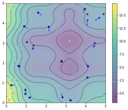
Positions of particles after one iteration
We can repeat the above code segment for multiple times and see how the particles explore. This is the result after the second iteration:
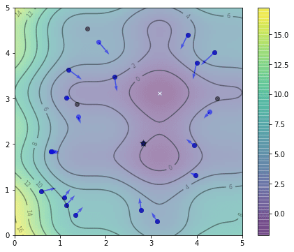
Positions of particles after two iterations
and this is after the 5th iteration, note that the position of $gbest$ as denoted by the star changed:
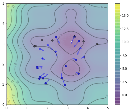
Positions of particles after 5 iterations
and after 20th iteration, we already very close to the optimal:
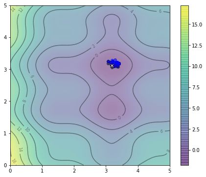
Positions of particles after 20 iterations
This is the animation showing how we find the optimal solution as the algorithm progressed. See if you may find some resemblance to the movement of a flock of birds:
Animation of particle movements
So how close is our solution? In this particular example, the global minimum we found by exhaustive search is at the coordinate $(3.182,3.131)$ and the one found by PSO algorithm above is at $(3.185,3.130)$.
Variations
All PSO algorithms are mostly the same as we mentioned above. In the above example, we set the PSO to run in a fixed number of iterations. It is trivial to set the number of iterations to run dynamically in response to the progress. For example, we can make it stop once we cannot see any update to the global best solution $gbest$ in a number of iterations.
Research on PSO were mostly on how to determine the hyperparameters $w$, $c_1$, and $c_2$ or varying their values as the algorithm progressed. For example, there are proposals making the inertia weight linear decreasing. There are also proposals trying to make the cognitive coefficient $c_1$ decreasing while the social coefficient $c_2$ increasing to bring more exploration at the beginning and more exploitation at the end. See, for example, Shi and Eberhart (1998) and Eberhart and Shi (2000).
Complete Example
It should be easy to see how we can change the above code to solve a higher dimensional objective function, or switching from minimization to maximization. The following is the complete example of finding the minimum point of the function $f(x,y)$ proposed above, together with the code to generate the plot animation:
|
1 2 3 4 5 6 7 8 9 10 11 12 13 14 15 16 17 18 19 20 21 22 23 24 25 26 27 28 29 30 31 32 33 34 35 36 37 38 39 40 41 42 43 44 45 46 47 48 49 50 51 52 53 54 55 56 57 58 59 60 61 62 63 64 65 66 67 68 69 70 71 72 73 74 75 76 77 78 79 |
import numpy as np import matplotlib.pyplot as plt from matplotlib.animation import FuncAnimation def f(x,y): "Objective function" return (x-3.14)**2 + (y-2.72)**2 + np.sin(3*x+1.41) + np.sin(4*y-1.73) # Compute and plot the function in 3D within [0,5]x[0,5] x, y = np.array(np.meshgrid(np.linspace(0,5,100), np.linspace(0,5,100))) z = f(x, y) # Find the global minimum x_min = x.ravel()[z.argmin()] y_min = y.ravel()[z.argmin()] # Hyper-parameter of the algorithm c1 = c2 = 0.1 w = 0.8 # Create particles n_particles = 20 np.random.seed(100) X = np.random.rand(2, n_particles) * 5 V = np.random.randn(2, n_particles) * 0.1 # Initialize data pbest = X pbest_obj = f(X[0], X[1]) gbest = pbest[:, pbest_obj.argmin()] gbest_obj = pbest_obj.min() def update(): "Function to do one iteration of particle swarm optimization" global V, X, pbest, pbest_obj, gbest, gbest_obj # Update params r1, r2 = np.random.rand(2) V = w * V + c1*r1*(pbest - X) + c2*r2*(gbest.reshape(-1,1)-X) X = X + V obj = f(X[0], X[1]) pbest[:, (pbest_obj >= obj)] = X[:, (pbest_obj >= obj)] pbest_obj = np.array([pbest_obj, obj]).min(axis=0) gbest = pbest[:, pbest_obj.argmin()] gbest_obj = pbest_obj.min() # Set up base figure: The contour map fig, ax = plt.subplots(figsize=(8,6)) fig.set_tight_layout(True) img = ax.imshow(z, extent=[0, 5, 0, 5], origin='lower', cmap='viridis', alpha=0.5) fig.colorbar(img, ax=ax) ax.plot([x_min], [y_min], marker='x', markersize=5, color="white") contours = ax.contour(x, y, z, 10, colors='black', alpha=0.4) ax.clabel(contours, inline=True, fontsize=8, fmt="%.0f") pbest_plot = ax.scatter(pbest[0], pbest[1], marker='o', color='black', alpha=0.5) p_plot = ax.scatter(X[0], X[1], marker='o', color='blue', alpha=0.5) p_arrow = ax.quiver(X[0], X[1], V[0], V[1], color='blue', width=0.005, angles='xy', scale_units='xy', scale=1) gbest_plot = plt.scatter([gbest[0]], [gbest[1]], marker='*', s=100, color='black', alpha=0.4) ax.set_xlim([0,5]) ax.set_ylim([0,5]) def animate(i): "Steps of PSO: algorithm update and show in plot" title = 'Iteration {:02d}'.format(i) # Update params update() # Set picture ax.set_title(title) pbest_plot.set_offsets(pbest.T) p_plot.set_offsets(X.T) p_arrow.set_offsets(X.T) p_arrow.set_UVC(V[0], V[1]) gbest_plot.set_offsets(gbest.reshape(1,-1)) return ax, pbest_plot, p_plot, p_arrow, gbest_plot anim = FuncAnimation(fig, animate, frames=list(range(1,50)), interval=500, blit=False, repeat=True) anim.save("PSO.gif", dpi=120, writer="imagemagick") print("PSO found best solution at f({})={}".format(gbest, gbest_obj)) print("Global optimal at f({})={}".format([x_min,y_min], f(x_min,y_min))) |
Further Reading
These are the original papers that proposed the particle swarm optimization, and the early research on refining its hyperparameters:
- Kennedy J. and Eberhart R. C. Particle swarm optimization. In Proceedings of the International Conference on Neural Networks; Institute of Electrical and Electronics Engineers. Vol. 4. 1995. pp. 1942–1948. DOI: 10.1109/ICNN.1995.488968
- Eberhart R. C. and Shi Y. Comparing inertia weights and constriction factors in particle swarm optimization. In Proceedings of the 2000 Congress on Evolutionary Computation (CEC ‘00). Vol. 1. 2000. pp. 84–88. DOI: 10.1109/CEC.2000.870279
- Shi Y. and Eberhart R. A modified particle swarm optimizer. In Proceedings of the IEEE International Conferences on Evolutionary Computation, 1998. pp. 69–73. DOI: 10.1109/ICEC.1998.699146
Summary
In this tutorial we learned:
- How particle swarm optimization works
- How to implement the PSO algorithm
- Some possible variations in the algorithm
As particle swarm optimization does not have a lot of hyper-parameters and very permissive on the objective function, it can be used to solve a wide range of problems.
Get a Handle on Modern Optimization Algorithms!
Develop Your Understanding of Optimization
...with just a few lines of python code
Discover how in my new Ebook:
Optimization for Machine Learning
It provides self-study tutorials with full working code on:
Gradient Descent, Genetic Algorithms, Hill Climbing, Curve Fitting, RMSProp, Adam,
and much more...
")


Very good article Jason. thanks for sharing.
We can use it to find and set the initial weights of a neural network to save training time. And use bep to find global minimum where weights are optimized and the error in minimum.
Gradient decent can do that but we have error vanishing issue and training time is a lot in complex networks, so instead of initializing the network with some random weights we can start with the optimized weights from pso and bep will do rest of the job.
I have done it on several projects and worked fine.
I agree, you can use it to initialize weights of neural networks, and hopefully train in less epochs. Can you tell if you have done it using some popular libraries like tensorflow or pytorch?
How to combine pso with ann Or with svm for regression task. Or any other machine learning algorithm.
I guess can we use loss function as object function .
Yes, you wrap the entire model as the objective function then apply your favorite optimization algorithm to it.
Thank you, sir. This article has been incredibly informative. Do you have an example illustrating how we can apply PSO to our ML model?
Hi Amr…The following resource is a great starting point:
https://link.springer.com/article/10.1007/s11831-021-09694-4
PSO is an optimization method. For example, you can use it to do search on optimal hyperparameters. Simply make your machine learning model as the objective function and apply PSO on the parameter, for example.
Adrian,
Outstanding article! Particle swarming techniques are becoming a big area of interest at work and this is a fantastic primer on the topic!
Glad you like it!
Thank you Jason! I have been searching for this for a long time to replace it instead of backprop.
Hope you like it!
Thank YOU!
Once again, you not only covered the topic very precisely but you also created an impressive demonstration on how the PSO algorithm functions. Hats off to you for breaking it down the way you did!!
Thanks. Glad you enjoyed it.
Can you explain this fancy boolean indexing?
pbest[:, (pbest_obj >= obj)] = X[:, (pbest_obj >= obj)]
If X is a vector, (X > n) will give you a boolean vector for “true” whenever element of X greater than n and “false” otherwise. Then Y[(X > n)] will select the elements from Y on the position that (X > n) is “true”. This essentially picks a sub-vector or sub-matrix from Y according to the boolean value.
Dear Adrian Tam
Thank you for your wonderful your blog and how to combine pso and machine learning algorithm in other dataset? like xgboost
Depends on why you want to do that. If you try to explore the hyperparameters for XGBoost, you can wrap your XGBoost model as a function, which the input are the hyperparameter, output is the score. Then feed this function into optimization to find the best-performing hyperparamters.
Adrian,
Good afternoon! If you have a minute, I’m wondering if you can help expand on what you have. Say I want to have the particles, instead of searching for the ‘x’, chase after a moving ‘x’. Is there a relatively efficient way to make that happen? It seems like I could keep the data initialization section the same for simplicity. Then, maybe define points of a square, for example, and use those four points for pbest_obj and gbest_obj?
This is a great piece of code! I’ve gotten a lot out of it by modifying the objective function and hyperparameters to get a good idea of how the algorithm works. Thank you very much for posting this and for your time!
Dear Adrian,
absolutely useful article. Especially the graphical part! I only noticed a very simple correction in the following line:
pbest_obj = np.array([pbest_obj, obj]).max(axis=0)
I guess max(axis=0) should change to min(axis=0) as we are going to find the minimum of the objective function. You already have corrected it in the “Complete Example” part.
Thanks again,
Great feedback Erfan!
How can I set the constraint and number of iterations?
Hi Betty…You may find the following of interest:
https://medium.com/swlh/particle-swarm-optimization-731d9fbb6923
same question here. is it at “animate(i)”? is the “i” the iteration?
Hi,
Thanks for the tutorial. Good job!
I am working on a dataset to find the accuracy of Hand Gesture classification using different algorithms like KNN and SVM (using the sklearn libraries in python). Now I have to optimize the accuracy found by the SVM using Particle Swarm optimization algorithm. But I don’t know where to begin with with this optimization problem following your guide to PSO.
I have my implementaion of SVM part done , and now I want to optimize it using the PSO.
Any help regarding this matter will be really appreciated. Or even if you can point me in the right direction, that would also be helpful.
Thanks again.
Hi Ryan…Please specify exactly what you are trying to accomplish and/or items from the tutorial that you are not clear how to apply.
Thanks for the answer,
I will try to explain from the beginning.
I have a dataset in a CSV format, that contains information about the hand gestures in the American sign language, extracted in the form of features and it contains decimal values(no strings). As a reference I have attached the reference to a paper for better understanding or explain what I am trying to do.
https://revistas.usal.es/index.php/2255-2863/article/view/ADCAIJ2021102123136
Now, I want to calculate that which ANN algorithm variant (like k nearest neighbours, Support Vector Machines, Naive Bayes, Decision Tree etc.) gives me the best accuracy on this dataset. So, using the built in libraries in Python(numpy, pandas, sklearn), I created a python code, split my data into training and testing, and applied the algorithms e.g. SVM on my dataset and got the accuracy of 75%. Now, I would like to improve this accuracy using optimization algorithms like PSO or Genetic Algorihtm. For that part I need help. Like.., how do I optimize the accuracy of SVM using particle swarm optimazation in the python code.
You have a sample PSO code in python above. How do I follow your example and get the best possible results for my dataset on which I have applied the SVM algortihm…?
Thanks again for taking your time out to read my comment.
Awaiting your kind response.
Thanks
How can i add constraints to the function?
Hi Monish…The following may be of interest:
https://www.cs.cinvestav.mx/~constraint/papers/eisci.pdf
Hi James,
Can you also please reply to my comment just above, if possible. Would really appreciate that.
Thanks a lot.
Hi James,
Can you please take some time to comment on my question that I asked above. Would really appreciate your help.
Thanks
Amazing demonstration, Thank you kind sir
a small problem under 3rd plot, in the code snippet I believe in line 9, max(axis=0) should be changed to min(axis=0), like the complete example code, line 42
much appreciated again, excellent explanation.
Do you have an example multiobjective problem using PSO (or another, like NSGA-III, or MOEA/D),
or perhaps using pyMoo, playpus, or jMetalPy?
Hi Keith…We do not currently have examples directly related to those concepts.
Do you have any suggestions, or references, on how PSO could be applied to a multi-objective optimisation problem please?
Hi Peter…The following dissertation is a great stating point:
https://core.ac.uk/download/pdf/48631978.pdf
Thank you very much , i have question please tell me how can i use this example to make optimization on schedule on Gantt chart.
Hi noor…You are very welcome! Please clarify the specific goals of your model and the nature of your input so that we may better assist you.
How do I apply the code above as an optimization to the Gantt Chart
Or, How can the code be combined with the Gantt chart?
؟؟؟؟ help me
I am need to use the code with Gantt chart scheduling of PSO method , how can i do it ??
Hi sara…the following resource may add clarity:
https://www.researchgate.net/publication/260087478_A_Particle_Swarm_Optimization_Algorithm_for_Scheduling_Against_Restrictive_Common_Due_Dates
thank you so much, it’s helpful but can I get the code for this pepper ?
***paper
Hi, I have a question when it comes to solving any optimization problem. I am currently working on the budget spend optimization for various medias. I have historical data in the format x1, x2, x3,x4 and y where x1, x2, x3 and x4 are the input variables and are the spend per channel and y is the output that is the total revenue achieved based on the spend of x1 + x2 + x3 + x4. The biggest question is how to derive the objective function from the historical performance data ? Could you please help me with this. I have been trying to figure out from the last few days but no luck yet. 🙁
Hi
I need to use pso to Model keras conv1d
How add this to model ? To optimize hyper prameter
Hi, I have been trying to solve the marketing spend optimization problem using cvxpy library. I have the input as x1,x2,x3 and x4 with output y. So, x1, x2,x3 and x4 are the spend per media channel (we have 4 channels) and then y is the total revenue achieved due to the x1 + x2 + x3 + x4 spend combined. I also have individual channel level revenue for all the 4 channels. Now my biggest challenge is how to derive the objective function to solve such problems ? Could you share any thoughts here or any guidance will be really very helpful.
Hi Siddharth…The following resource should be of interest:
https://machinelearningmastery.com/optimization-for-machine-learning-crash-course/
Hi
I need to use pso to Model keras conv1d
How add this to model ? To optimize hyper prameter
are you have pyton code model for this case but using simulated annealing algorithm
Hi Firman…The following resource may be of interest:
https://machinelearningmastery.com/simulated-annealing-from-scratch-in-python/
Can you help me by discussing All Members Based Optimization technique in step by step with a small example. Thanks in advance.
Hi Lakshmi…The following resource may be of interest to you:
https://www.techscience.com/cmc/v70n2/44661
Hi
Thanks ???? for everything
I ask how can use pso to optimize Hyperprameter filter for cnn1d?? What’s code for this if u can helpe me please
It may not be easily done in a few lines of code but I can share with you the method: Create a function for the CNN, such that it takes hyperparameter as input and some evaluation metric as output (e.g., a MSE of a fixed test dataset). In the function, you build the CNN using the hyperparameter, do the training, and perform evaluation. Then apply PSO on this function which the PSO is to change the hyperparameter and observe the function’s output.
Note that, since each iteration in PSO is to create multiple CNN and evaluate it, there’s a lot of computation involved. You need to be patient.
Thanks you, Json, it’s an awsome article, and I began to learn the algorithm from your work.
I am curious about the code below:
python

pbest_obj = np.array([pbest_obj, obj]).max(axis=0)
I think it’s maybe a mistabke, and the function you want to use is min(axis=0)
Hi Dean…You are very welcome! Please elborate on why you disagree with the original code.
This website is by far the best website for learning optimization, Python, and machine learning. I found that there are at least 12 optimization algorithms in Python. Is there any code for ICA? Imperialist competitive algorithm?
Hi MBT…we greatly appreciate your feedback! The following location is a great starting point for all of our content.
https://machinelearningmastery.com/start-here/
Thank you, Adrian Tam, for this post. It is really helpful. I have a question. Could you please help me apply the PSO algorithm to the kullback-leibler divergence function?
Hi Mebarka…The following resource is a great starting point:
http://dx.doi.org/10.1371/journal.pcbi.1006694
Thank you James for the document
Hi james,
previously i read many topics in your blog. All are very unique in explanation. I understood the concept of PSO. I need some help to apply PSO for a customized U-net model. Suggest me how to write objective function for reducing the complexity and what should be the parameters for PSO that i need pass. what parameters to initialize the population
Hi Nagamani…Below is a simplified example of how you can implement Particle Swarm Optimization (PSO) for optimizing hyperparameters of a U-Net model in Python using the
pyswarmlibrary for optimization andtensorflowfor building and training the U-Net model. This example assumes a simple binary image segmentation task.pythonimport numpy as np
import tensorflow as tf
from pyswarm import pso
# Define U-Net model architecture
def unet_model(input_shape, num_filters):
inputs = tf.keras.layers.Input(input_shape)
# Encoder
conv1 = tf.keras.layers.Conv2D(num_filters, 3, activation='relu', padding='same')(inputs)
pool1 = tf.keras.layers.MaxPooling2D(pool_size=(2, 2))(conv1)
# Decoder
conv2 = tf.keras.layers.Conv2D(num_filters, 3, activation='relu', padding='same')(pool1)
up1 = tf.keras.layers.UpSampling2D(size=(2, 2))(conv2)
# Output
outputs = tf.keras.layers.Conv2D(1, 1, activation='sigmoid')(up1)
model = tf.keras.Model(inputs=inputs, outputs=outputs)
return model
# Objective function to be minimized by PSO
def objective_function(params):
# Hyperparameters to optimize
input_shape = (256, 256, 1)
num_filters = int(params[0])
# Build U-Net model
model = unet_model(input_shape, num_filters)
# Compile model
model.compile(optimizer='adam', loss='binary_crossentropy', metrics=['accuracy'])
# Dummy data (replace with your actual data)
x_train = np.random.rand(100, 256, 256, 1)
y_train = np.random.randint(2, size=(100, 256, 256, 1))
# Train model
model.fit(x_train, y_train, epochs=3, batch_size=32, verbose=0)
# Evaluate model
loss, _ = model.evaluate(x_train, y_train, verbose=0)
return loss
# Define search space bounds for num_filters
lb = [16] # Lower bound for num_filters
ub = [64] # Upper bound for num_filters
# Run PSO optimization
num_particles = 10
max_iterations = 20
best_params, _ = pso(objective_function, lb, ub, swarmsize=num_particles, maxiter=max_iterations)
print("Best number of filters:", int(best_params[0]))
In this example:
– We define the U-Net model architecture with a simple encoder-decoder structure.
– The objective function
objective_functiontakes the number of filters in the U-Net model as input, builds the model with the given hyperparameters, trains it, and returns the validation loss.– We use the
pyswarm.psofunction to optimize the objective function and find the best hyperparameters.– The search space is defined by the lower bound (
lb) and upper bound (ub) for the number of filters.Make sure to replace the dummy data with your actual dataset for training and evaluation. Additionally, you may need to adjust the model architecture and objective function based on your specific task and requirements.
Thank you so much James.
Can you even suggest me how to combine genetic algorithm with a particle swarm optimization algorithm for hyper parameter tuning.