Function optimization is a foundational area of study and the techniques are used in almost every quantitative field.
Importantly, function optimization is central to almost all machine learning algorithms, and predictive modeling projects. As such, it is critical to understand what function optimization is, the terminology used in the field, and the elements that constitute a function optimization problem.
In this tutorial, you will discover a gentle introduction to function optimization.
After completing this tutorial, you will know:
- The three elements of function optimization as candidate solutions, objective functions, and cost.
- The conceptualization of function optimization as navigating a search space and response surface.
- The difference between global optima and local optima when solving a function optimization problem.
Kick-start your project with my new book Optimization for Machine Learning, including step-by-step tutorials and the Python source code files for all examples.
Let’s get started.
A Gentle Introduction to Function Optimization
Photo by USFS, Interior West FIA, some rights reserved.
Tutorial Overview
This tutorial is divided into four parts; they are:
- Function Optimization
- Candidate Solutions
- Objective Functions
- Evaluation Costs
Function Optimization
Function optimization is a subfield of mathematics, and in modern times is addressed using numerical computing methods.
Continuous function optimization (“function optimization” here for short) belongs to a broader field of study called mathematical optimization.
It is distinct from other types of optimization as it involves finding optimal candidate solutions composed of numeric input variables, as opposed to candidate solutions composed of sequences or combinations (e.g. combinatorial optimization).
Function optimization is a widely used tool bag of techniques employed in practically all scientific and engineering disciplines.
People optimize. Investors seek to create portfolios that avoid excessive risk while achieving a high rate of return. […] Optimization is an important tool in decision science and in the analysis of physical systems.
— Page 2, Numerical Optimization, 2006.
It plays a central role in machine learning, as almost all machine learning algorithms use function optimization to fit a model to a training dataset.
For example, fitting a line to a collection of points requires solving an optimization problem. As does fitting a linear regression or a neural network model on a training dataset.
In this way, optimization provides a tool to adapt a general model to a specific situation. Learning is treated as an optimization or search problem.
Practically, function optimization describes a class of problems for finding the input to a given function that results in the minimum or maximum output from the function.
The objective depends on certain characteristics of the system, called variables or unknowns. Our goal is to find values of the variables that optimize the objective.
— Page 2, Numerical Optimization, 2006.
Function Optimization involves three elements: the input to the function (e.g. x), the objective function itself (e.g. f()) and the output from the function (e.g. cost).
- Input (x): The input to the function to be evaluated, e.g. a candidate solution.
- Function (f()): The objective function or target function that evaluates inputs.
- Cost: The result of evaluating a candidate solution with the objective function, minimized or maximized.
Let’s take a closer look at each element in turn.
Want to Get Started With Optimization Algorithms?
Take my free 7-day email crash course now (with sample code).
Click to sign-up and also get a free PDF Ebook version of the course.
Candidate Solutions
A candidate solution is a single input to the objective function.
The form of a candidate solution depends on the specifics of the objective function. It may be a single floating point number, a vector of numbers, a matrix of numbers, or as complex as needed for the specific problem domain.
Most commonly, vectors of numbers. For a test problem, the vector represents the specific values of each input variable to the function (x = x1, x2, x3, …, xn). For a machine learning model, the vector may represent model coefficients or weights.
Mathematically speaking, optimization is the minimization or maximization of a function subject to constraints on its variables.
— Page 2, Numerical Optimization, 2006.
There may be constraints imposed by the problem domain or the objective function on the candidate solutions. This might include aspects such as:
- The number of variables (1, 20, 1,000,000, etc.)
- The data type of variables (integer, binary, real-valued, etc.)
- The range of accepted values (between 0 and 1, etc.)
Importantly, candidate solutions are discrete and there are many of them.
The universe of candidate solutions may be vast, too large to enumerate. Instead, the best we can do is sample candidate solutions in the search space. As a practitioner, we seek an optimization algorithm that makes the best use of the information available about the problem to effectively sample the search space and locate a good or best candidate solution.
- Search Space: Universe of candidate solutions defined by the number, type, and range of accepted inputs to the objective function.
Finally, candidate solutions can be rank-ordered based on their evaluation by the objective function, meaning that some are better than others.
Objective Functions
The objective function is specific to the problem domain.
It may be a test function, e.g. a well-known equation with a specific number of input variables, the calculation of which returns the cost of the input. The optima of test functions are known, allowing algorithms to be compared based on their ability to navigate the search space efficiently.
In machine learning, the objective function may involve plugging the candidate solution into a model and evaluating it against a portion of the training dataset, and the cost may be an error score, often called the loss of the model.
The objective function is easy to define, although expensive to evaluate. Efficiency in function optimization refers to minimizing the total number of function evaluations.
Although the objective function is easy to define, it may be challenging to optimize. The difficulty of an objective function may range from being able to analytically solve the function directly using calculus or linear algebra (easy), to using a local search algorithm (moderate), to using a global search algorithm (hard).
The difficulty of an objective function is based on how much is known about the function. This often cannot be determined by simply reviewing the equation or code for evaluating candidate solutions. Instead, it refers to the structure of the response surface.
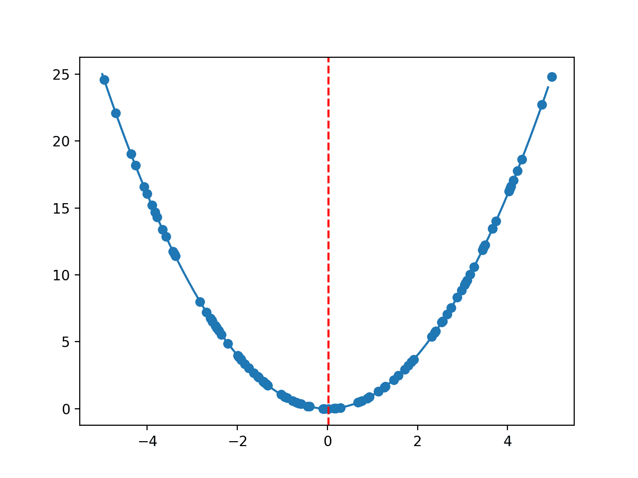
The response surface (or search landscape) is the geometrical structure of the cost in relation to the search space of candidate solutions. For example, a smooth response surface suggests that small changes to the input (candidate solutions) result in small changes to the output (cost) from the objective function.
- Response Surface: Geometrical properties of the cost from the objective function in response to changes to the candidate solutions.
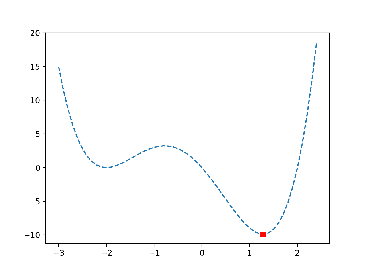
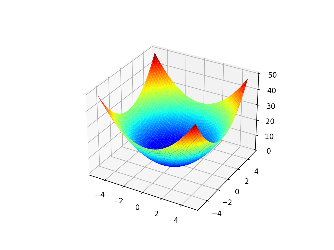
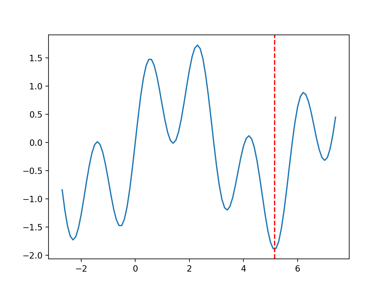
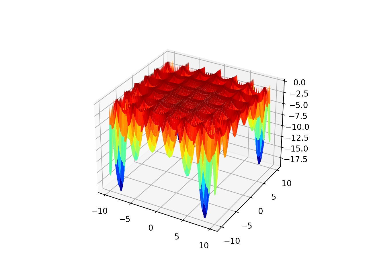
The response surface can be visualized in low dimensions, e.g. for candidate solutions with one or two input variables. A one-dimensional input can be plotted as a 2D scatter plot with input values on the x-axis and the cost on the y-axis. A two-dimensional input can be plotted as a 3D surface plot with input variables on the x and y-axis, and the height of the surface representing the cost.
In a minimization problem, poor solutions would be represented as hills in the response surface and good solutions would be represented by valleys. This would be inverted for maximizing problems.
The structure and shape of this response surface determine the difficulty an algorithm will have in navigating the search space to a solution.
The complexity of real objective functions means we cannot analyze the surface analytically, and the high dimensionality of the inputs and computational cost of function evaluations makes mapping and plotting real objective functions intractable.
Evaluation Costs
The cost of a candidate solution is almost always a single real-valued number.
The scale of the cost values will vary depending on the specifics of the objective function. In general, the only meaningful comparison of cost values is to other cost values calculated by the same objective function.
The minimum or maximum output from the function is called the optima of the function, typically simplified to simply the minimum. Any function we wish to maximize can be converted to minimizing by adding a negative sign to the front of the cost returned from the function.
In global optimization, the true global solution of the optimization problem is found; the compromise is efficiency. The worst-case complexity of global optimization methods grows exponentially with the problem sizes …
— Page 10, Convex Optimization, 2004.
An objective function may have a single best solution, referred to as the global optimum of the objective function. Alternatively, the objective function may have many global optima, in which case we may be interested in locating one or all of them.
Many numerical optimization methods seek local minima. Local minima are locally optimal, but we do not generally know whether a local minimum is a global minimum.
— Page 8, Algorithms for Optimization, 2019.
In addition to a global optima, a function may have local optima, which are good candidate solutions that may be relatively easy to locate, but not as good as the global optima. Local optima may appear to be global optima to a search algorithm, e.g. may be in a valley of the response surface, in which case we might refer to them as deceptive as the algorithm will easily locate them and get stuck, failing to locate the global optima.
- Global Optima: The candidate solution with the best cost from the objective function.
- Local Optima. Candidate solutions are good but not as good as the global optima.
The relative nature of cost values means that a baseline in performance on challenging problems can be established using a naive search algorithm (e.g. random) and “goodness” of optimal solutions found by more sophisticated search algorithms can be compared relative to the baseline.
Candidate solutions are often very simple to describe and very easy to construct. The challenging part of function optimization is evaluating candidate solutions.
Solving a function optimization problem or objective function refers to finding the optima. The whole goal of the project is to locate a specific candidate solution with a good or best cost, give the time and resources available. In simple and moderate problems, we may be able to locate the optimal candidate solution exactly and have some confidence that we have done so.
Many algorithms for nonlinear optimization problems seek only a local solution, a point at which the objective function is smaller than at all other feasible nearby points. They do not always find the global solution, which is the point with lowest function value among all feasible points. Global solutions are needed in some applications, but for many problems they are difficult to recognize and even more difficult to locate.
— Page 6, Numerical Optimization, 2006.
On more challenging problems, we may be happy with a relatively good candidate solution (e.g. good enough) given the time available for the project.
Further Reading
This section provides more resources on the topic if you are looking to go deeper.
Books
- Algorithms for Optimization, 2019.
- Convex Optimization, 2004.
- Numerical Optimization, 2006.
Articles
Summary
In this tutorial, you discovered a gentle introduction to function optimization.
Specifically, you learned:
- The three elements of function optimization as candidate solutions, objective functions and cost.
- The conceptualization of function optimization as navigating a search space and response surface.
- The difference between global optima and local optima when solving a function optimization problem.
Do you have any questions?
Ask your questions in the comments below and I will do my best to answer.


Small comment – optima is a plural, hence it should be local optima but a global optimum. Or perhaps many global optima. But not a global optima.
Thanks.