Function optimization is a field of study that seeks an input to a function that results in the maximum or minimum output of the function.
There are a large number of optimization algorithms and it is important to study and develop intuitions for optimization algorithms on simple and easy-to-visualize test functions.
Two-dimensional functions take two input values (x and y) and output a single evaluation of the input. They are among the simplest types of test functions to use when studying function optimization. The benefit of two-dimensional functions is that they can be visualized as a contour plot or surface plot that shows the topography of the problem domain with the optima and samples of the domain marked with points.
In this tutorial, you will discover standard two-dimensional functions you can use when studying function optimization.
Kick-start your project with my new book Optimization for Machine Learning, including step-by-step tutorials and the Python source code files for all examples.
Let’s get started.
Two-Dimensional (2D) Test Functions for Function Optimization
Photo by DomWphoto, some rights reserved.
Tutorial Overview
A two-dimensional function is a function that takes two input variables and computes the objective value.
We can think of the two input variables as two axes on a graph, x and y. Each input to the function is a single point on the graph and the outcome of the function can be taken as the height on the graph.
This allows the function to be conceptualized as a surface and we can characterize the function based on the structure of the surface. For example, hills for input points that result in large relative outcomes of the objective function and valleys for input points that result in small relative outcomes of the objective function.
A surface may have one major feature or global optima, or it may have many with lots of places for an optimization to get stuck. The surface may be smooth, noisy, convex, and all manner of other properties that we may care about when testing optimization algorithms.
There are many different types of simple two-dimensional test functions we could use.
Nevertheless, there are standard test functions that are commonly used in the field of function optimization. There are also specific properties of test functions that we may wish to select when testing different algorithms.
We will explore a small number of simple two-dimensional test functions in this tutorial and organize them by their properties with two different groups; they are:
- Unimodal Functions
- Unimodal Function 1
- Unimodal Function 2
- Unimodal Function 3
- Multimodal Functions
- Multimodal Function 1
- Multimodal Function 2
- Multimodal Function 3
Each function will be presented using Python code with a function implementation of the target objective function and a sampling of the function that is shown as a surface plot.
All functions are presented as a minimization function, e.g. find the input that results in the minimum (smallest value) output of the function. Any maximizing function can be made a minimization function by adding a negative sign to all output. Similarly, any minimizing function can be made maximizing in the same way.
I did not invent these functions; they are taken from the literature. See the further reading section for references.
You can then choose and copy-paste the code one or more functions to use in your own project to study or compare the behavior of optimization algorithms.
Unimodal Functions
Unimodal means that the function has a single global optima.
A unimodal function may or may not be convex. A convex function is a function where a line can be drawn between any two points in the domain and the line remains in the domain. For a two-dimensional function shown as a contour or surface plot, this means the function has a bowl shape and the line between two remains above or in the bowl.
Let’s look at a few examples of unimodal functions.
Unimodal Function 1
The range is bounded to -5.0 and 5.0 and one global optimal at [0.0, 0.0].
|
1 2 3 4 5 6 7 8 9 10 11 12 13 14 15 16 17 18 19 20 21 22 23 24 25 |
# unimodal test function from numpy import arange from numpy import meshgrid from matplotlib import pyplot from mpl_toolkits.mplot3d import Axes3D # objective function def objective(x, y): return x**2.0 + y**2.0 # define range for input r_min, r_max = -5.0, 5.0 # sample input range uniformly at 0.1 increments xaxis = arange(r_min, r_max, 0.1) yaxis = arange(r_min, r_max, 0.1) # create a mesh from the axis x, y = meshgrid(xaxis, yaxis) # compute targets results = objective(x, y) # create a surface plot with the jet color scheme figure = pyplot.figure() axis = figure.gca(projection='3d') axis.plot_surface(x, y, results, cmap='jet') # show the plot pyplot.show() |
Running the example creates a surface plot of the function.
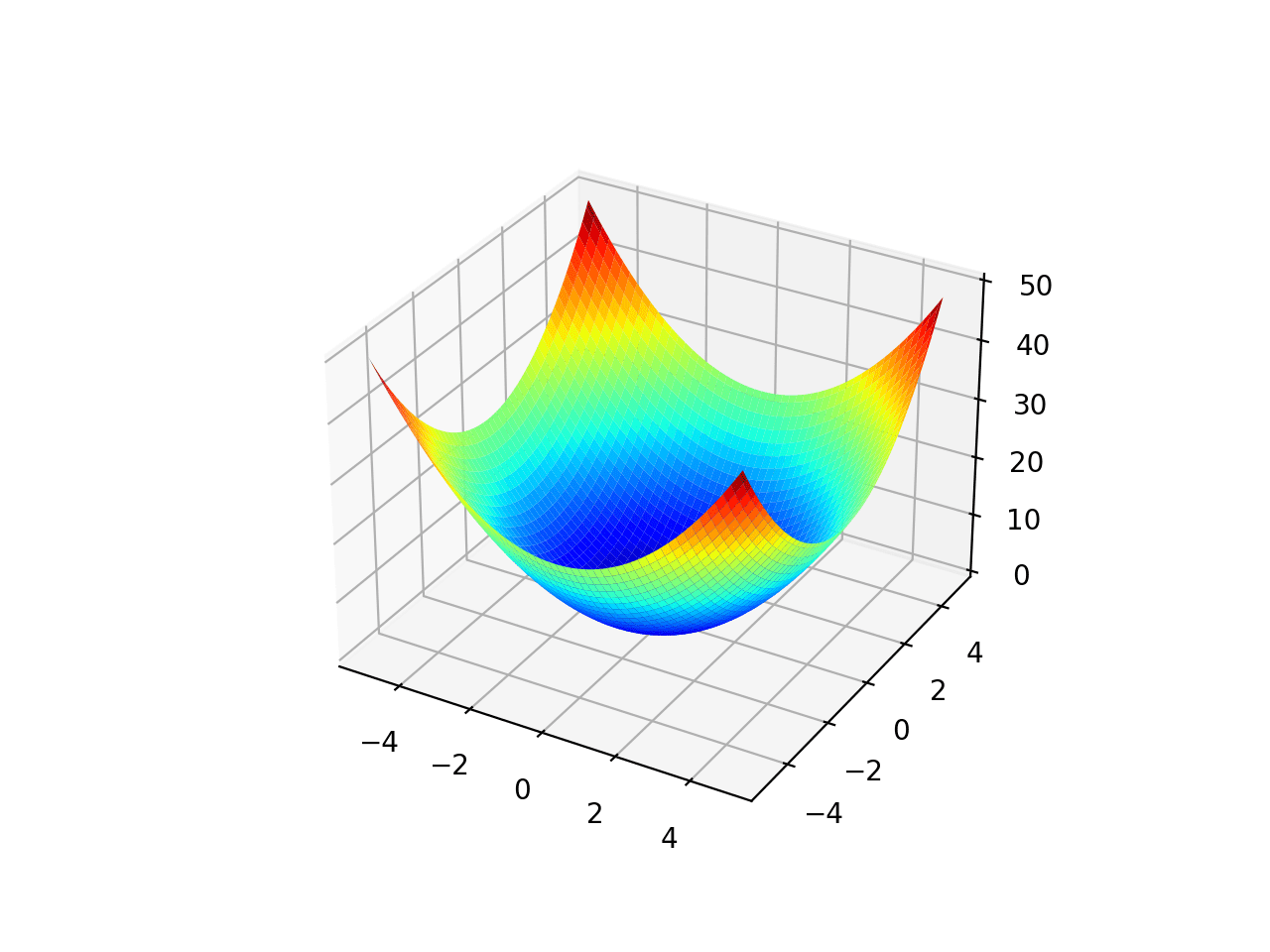
Surface Plot of Unimodal Optimization Function 1
Unimodal Function 2
The range is bounded to -10.0 and 10.0 and one global optimal at [0.0, 0.0].
|
1 2 3 4 5 6 7 8 9 10 11 12 13 14 15 16 17 18 19 20 21 22 23 24 25 |
# unimodal test function from numpy import arange from numpy import meshgrid from matplotlib import pyplot from mpl_toolkits.mplot3d import Axes3D # objective function def objective(x, y): return 0.26 * (x**2 + y**2) - 0.48 * x * y # define range for input r_min, r_max = -10.0, 10.0 # sample input range uniformly at 0.1 increments xaxis = arange(r_min, r_max, 0.1) yaxis = arange(r_min, r_max, 0.1) # create a mesh from the axis x, y = meshgrid(xaxis, yaxis) # compute targets results = objective(x, y) # create a surface plot with the jet color scheme figure = pyplot.figure() axis = figure.gca(projection='3d') axis.plot_surface(x, y, results, cmap='jet') # show the plot pyplot.show() |
Running the example creates a surface plot of the function.
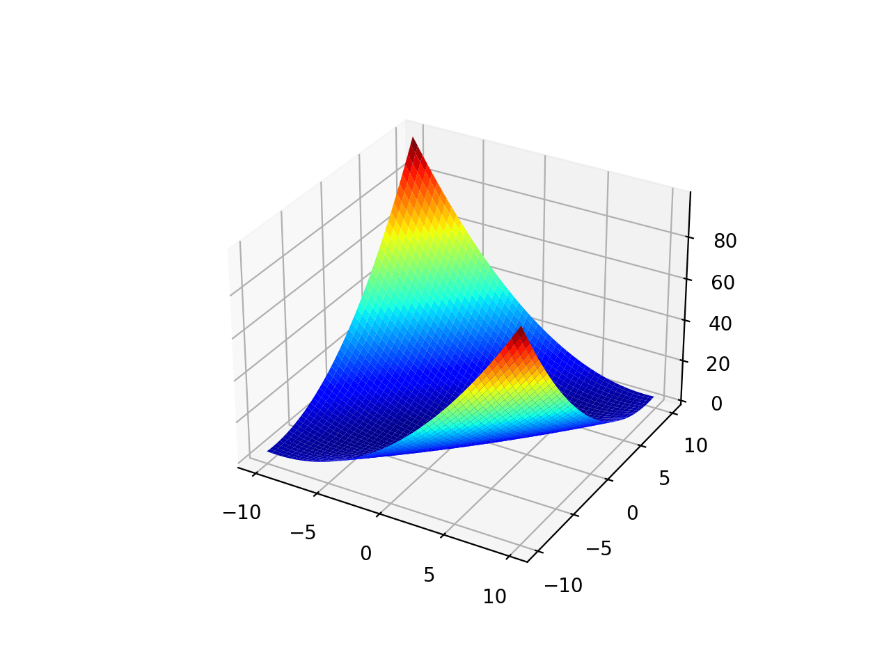
Surface Plot of Unimodal Optimization Function 2
Unimodal Function 3
The range is bounded to -10.0 and 10.0 and one global optimal at [pi, pi]. This function is known as Easom’s function.
|
1 2 3 4 5 6 7 8 9 10 11 12 13 14 15 16 17 18 19 20 21 22 23 24 25 26 27 28 |
# unimodal test function from numpy import cos from numpy import exp from numpy import pi from numpy import arange from numpy import meshgrid from matplotlib import pyplot from mpl_toolkits.mplot3d import Axes3D # objective function def objective(x, y): return -cos(x) * cos(y) * exp(-((x - pi)**2 + (y - pi)**2)) # define range for input r_min, r_max = -10, 10 # sample input range uniformly at 0.01 increments xaxis = arange(r_min, r_max, 0.01) yaxis = arange(r_min, r_max, 0.01) # create a mesh from the axis x, y = meshgrid(xaxis, yaxis) # compute targets results = objective(x, y) # create a surface plot with the jet color scheme figure = pyplot.figure() axis = figure.gca(projection='3d') axis.plot_surface(x, y, results, cmap='jet') # show the plot pyplot.show() |
Running the example creates a surface plot of the function.
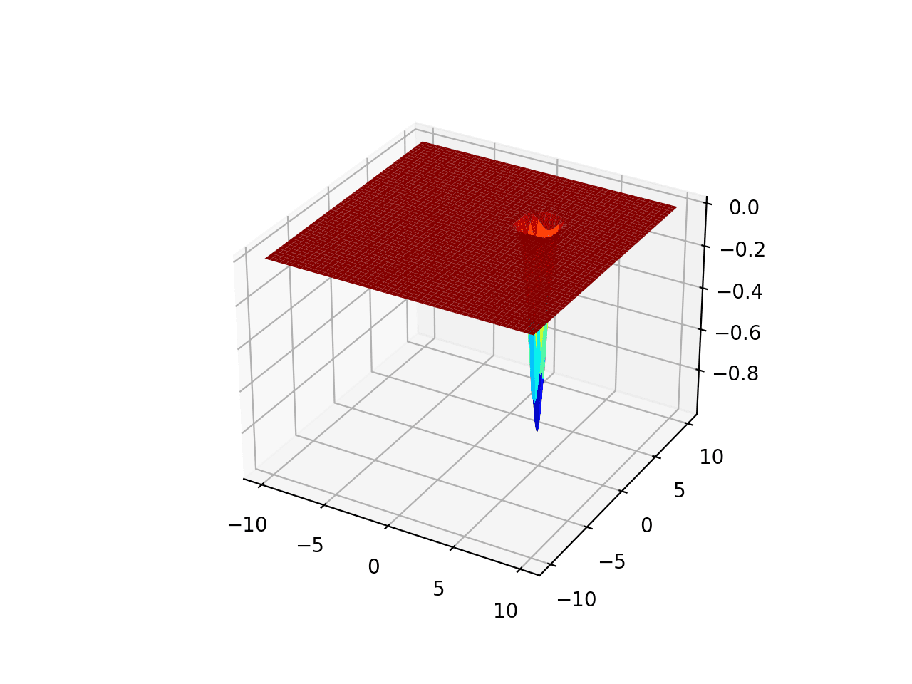
Surface Plot of Unimodal Optimization Function 3
Want to Get Started With Optimization Algorithms?
Take my free 7-day email crash course now (with sample code).
Click to sign-up and also get a free PDF Ebook version of the course.
Multimodal Functions
A multi-modal function means a function with more than one “mode” or optima (e.g. valley).
Multimodal functions are non-convex.
There may be one global optima and one or more local or deceptive optima. Alternately, there may be multiple global optima, i.e. multiple different inputs that result in the same minimal output of the function.
Let’s look at a few examples of multimodal functions.
Multimodal Function 1
The range is bounded to -5.0 and 5.0 and one global optimal at [0.0, 0.0]. This function is known as Ackley’s function.
|
1 2 3 4 5 6 7 8 9 10 11 12 13 14 15 16 17 18 19 20 21 22 23 24 25 26 27 28 29 30 |
# multimodal test function from numpy import arange from numpy import exp from numpy import sqrt from numpy import cos from numpy import e from numpy import pi from numpy import meshgrid from matplotlib import pyplot from mpl_toolkits.mplot3d import Axes3D # objective function def objective(x, y): return -20.0 * exp(-0.2 * sqrt(0.5 * (x**2 + y**2))) - exp(0.5 * (cos(2 * pi * x) + cos(2 * pi * y))) + e + 20 # define range for input r_min, r_max = -5.0, 5.0 # sample input range uniformly at 0.1 increments xaxis = arange(r_min, r_max, 0.1) yaxis = arange(r_min, r_max, 0.1) # create a mesh from the axis x, y = meshgrid(xaxis, yaxis) # compute targets results = objective(x, y) # create a surface plot with the jet color scheme figure = pyplot.figure() axis = figure.gca(projection='3d') axis.plot_surface(x, y, results, cmap='jet') # show the plot pyplot.show() |
Running the example creates a surface plot of the function.
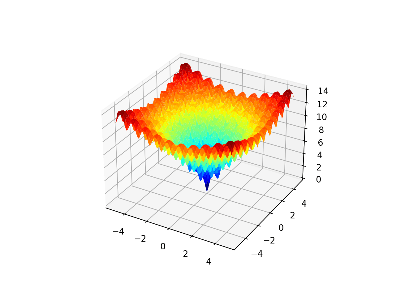
Surface Plot of Multimodal Optimization Function 1
Multimodal Function 2
The range is bounded to -5.0 and 5.0 and the function as four global optima at [3.0, 2.0], [-2.805118, 3.131312], [-3.779310, -3.283186], [3.584428, -1.848126]. This function is known as Himmelblau’s function.
|
1 2 3 4 5 6 7 8 9 10 11 12 13 14 15 16 17 18 19 20 21 22 23 24 25 |
# multimodal test function from numpy import arange from numpy import meshgrid from matplotlib import pyplot from mpl_toolkits.mplot3d import Axes3D # objective function def objective(x, y): return (x**2 + y - 11)**2 + (x + y**2 -7)**2 # define range for input r_min, r_max = -5.0, 5.0 # sample input range uniformly at 0.1 increments xaxis = arange(r_min, r_max, 0.1) yaxis = arange(r_min, r_max, 0.1) # create a mesh from the axis x, y = meshgrid(xaxis, yaxis) # compute targets results = objective(x, y) # create a surface plot with the jet color scheme figure = pyplot.figure() axis = figure.gca(projection='3d') axis.plot_surface(x, y, results, cmap='jet') # show the plot pyplot.show() |
Running the example creates a surface plot of the function.
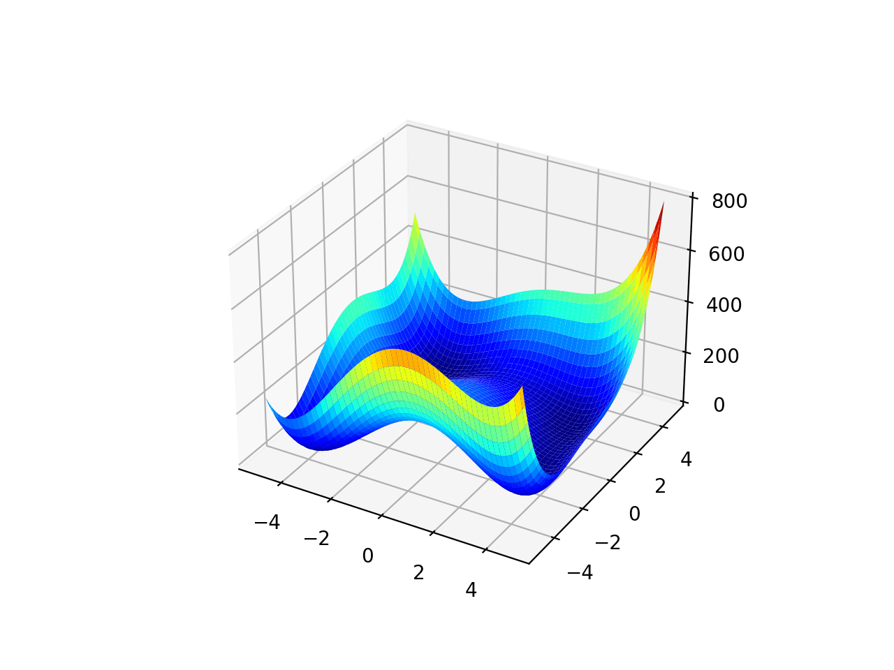
Surface Plot of Multimodal Optimization Function 2
Multimodal Function 3
The range is bounded to -10.0 and 10.0 and the function as four global optima at [8.05502, 9.66459], [-8.05502, 9.66459], [8.05502, -9.66459], [-8.05502, -9.66459]. This function is known as Holder’s table function.
|
1 2 3 4 5 6 7 8 9 10 11 12 13 14 15 16 17 18 19 20 21 22 23 24 25 26 27 28 29 30 31 32 |
# multimodal test function from numpy import arange from numpy import exp from numpy import sqrt from numpy import cos from numpy import sin from numpy import e from numpy import pi from numpy import absolute from numpy import meshgrid from matplotlib import pyplot from mpl_toolkits.mplot3d import Axes3D # objective function def objective(x, y): return -absolute(sin(x) * cos(y) * exp(absolute(1 - (sqrt(x**2 + y**2)/pi)))) # define range for input r_min, r_max = -10.0, 10.0 # sample input range uniformly at 0.1 increments xaxis = arange(r_min, r_max, 0.1) yaxis = arange(r_min, r_max, 0.1) # create a mesh from the axis x, y = meshgrid(xaxis, yaxis) # compute targets results = objective(x, y) # create a surface plot with the jet color scheme figure = pyplot.figure() axis = figure.gca(projection='3d') axis.plot_surface(x, y, results, cmap='jet') # show the plot pyplot.show() |
Running the example creates a surface plot of the function.
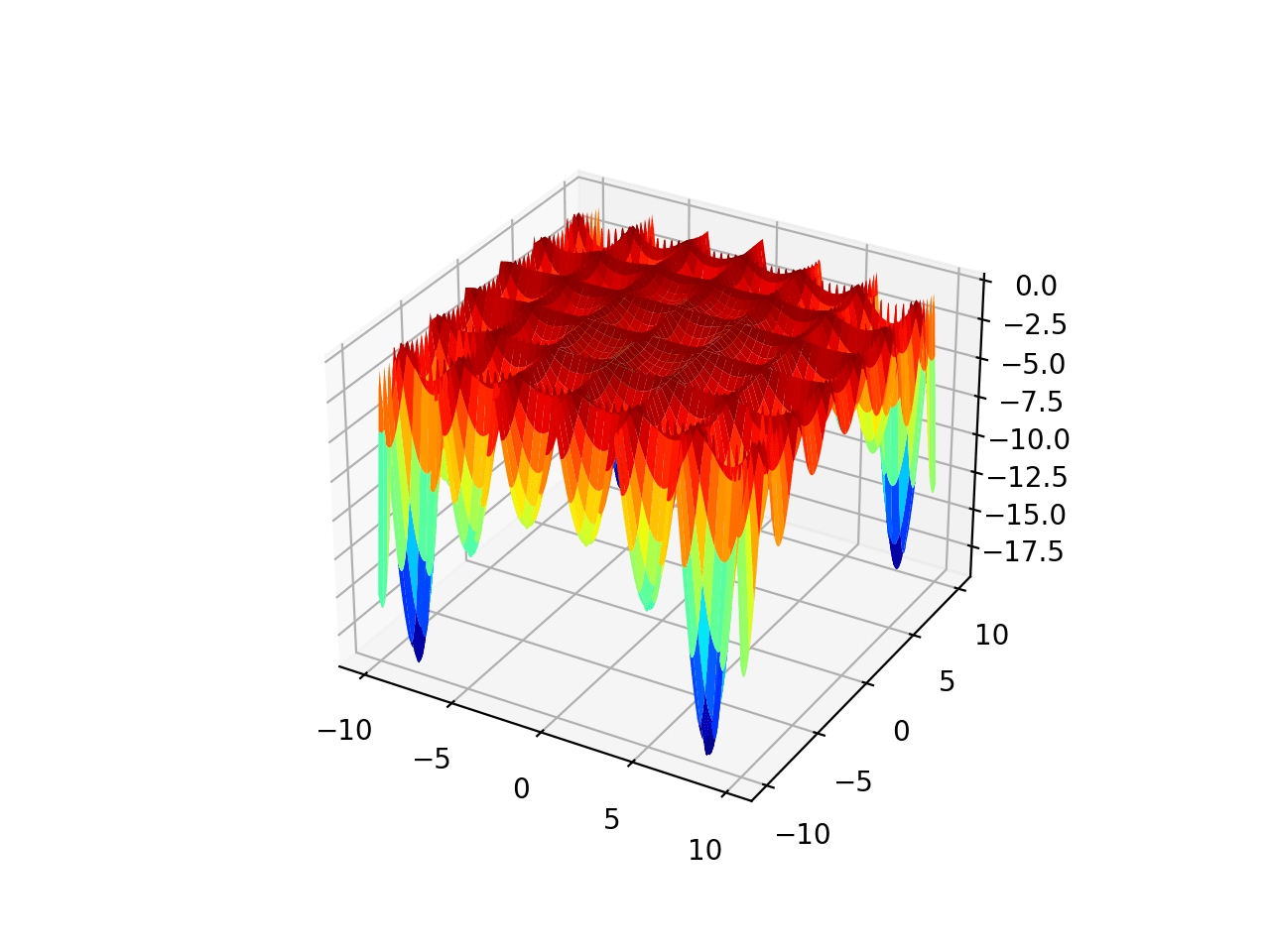
Surface Plot of Multimodal Optimization Function 3
Further Reading
This section provides more resources on the topic if you are looking to go deeper.
Articles
- Test functions for optimization, Wikipedia.
- Virtual Library of Simulation Experiments: Test Functions and Datasets
- Test Functions Index
- GEA Toolbox – Examples of Objective Functions
Summary
In this tutorial, you discovered standard two-dimensional functions you can use when studying function optimization.
Are you using any of the above functions?
Let me know which one in the comments below.
Do you have any questions?
Ask your questions in the comments below and I will do my best to answer.
Get a Handle on Modern Optimization Algorithms!

Develop Your Understanding of Optimization
...with just a few lines of python code
Discover how in my new Ebook:
Optimization for Machine Learning
It provides self-study tutorials with full working code on:
Gradient Descent, Genetic Algorithms, Hill Climbing, Curve Fitting, RMSProp, Adam,
and much more...
 Test Functions for Function Optimization")


Thanks for this awesome addition. But with optimization algorithms, there be one solution to be passed to this function. How to accomplish that? and how to plot these benchmarks given only a solution that is outputted in an algorithm trial?
Thanks!
You’re welcome.
The optimization algorithm will trial many candidate solutions against the objective function.
This can help you visualize solutions:
https://machinelearningmastery.com/visualization-for-function-optimization-in-python/
Hi, for Easom’s function should the location of the global minimum not be [pi,pi]? I
I think you’re right. Thanks!
https://en.wikipedia.org/wiki/Test_functions_for_optimization
What is the best algorithm for optimizing the cutting of two-dimensional plates?
Algorithm with the least amount of waste, I want to use this algorithm to calculate the MDF cut
Perhaps try a suite of algorithms and discover what works well or best for your objective problem.
Why not try CNN-LSTM?
in eggholder,
i want to calculate inputs on specific values …
like if im passing output=-959.6
it will gives input =[512,404]
kindly tell me how it possible
You are talking about reverse optimization, or inverting the problem. I don’t believe it is possible/tractable.