Optimization involves finding the inputs to an objective function that result in the minimum or maximum output of the function.
The open-source Python library for scientific computing called SciPy provides a suite of optimization algorithms. Many of the algorithms are used as a building block in other algorithms, most notably machine learning algorithms in the scikit-learn library.
These optimization algorithms can be used directly in a standalone manner to optimize a function. Most notably, algorithms for local search and algorithms for global search, the two main types of optimization you may encounter on a machine learning project.
In this tutorial, you will discover optimization algorithms provided by the SciPy library.
After completing this tutorial, you will know:
- The SciPy library provides a suite of different optimization algorithms for different purposes.
- The local search optimization algorithms available in SciPy.
- The global search optimization algorithms available in SciPy.
Kick-start your project with my new book Optimization for Machine Learning, including step-by-step tutorials and the Python source code files for all examples.
Let’s get started.
Function Optimization With SciPy
Photo by Manoel Lemos, some rights reserved.
Tutorial Overview
This tutorial is divided into three parts; they are:
- Optimization With SciPy
- Local Search With SciPy
- Global Search With SciPy
Optimization With SciPy
The Python SciPy open-source library for scientific computing provides a suite of optimization techniques.
Many of the algorithms are used as building blocks for other algorithms within the SciPy library, as well as machine learning libraries such as scikit-learn.
Before we review specific techniques, let’s look at the types of algorithms provided by the library.
They are:
- Scalar Optimization: Optimization of a convex single variable function.
- Local Search: Optimization of a unimodal multiple variable function.
- Global Search: Optimization of a multimodal multiple variable function.
- Least Squares: Solve linear and non-linear least squares problems.
- Curve Fitting: Fit a curve to a data sample.
- Root Finding: Find the root (input that gives an output of zero) of a function.
- Linear Programming: Linear optimization subject to constraints.
All algorithms assume the objective function that is being optimized is a minimization function. If your function is maximizing, it can be converted to minimizing by adding a negative sign to values returned from your objective function.
In addition to the above list, the library also provides utility functions used by some of the algorithms, as well as the Rosenbrock test problem.
For a good overview of the capabilities of the SciPy library for optimization, see:
Now that we have a high-level idea of the types of optimization techniques supported by the library, let’s take a closer look at two groups of algorithms we are more likely to use in applied machine learning. They are local search and global search.
Want to Get Started With Optimization Algorithms?
Take my free 7-day email crash course now (with sample code).
Click to sign-up and also get a free PDF Ebook version of the course.
Local Search With SciPy
Local search, or local function optimization, refers to algorithms that seek the input to a function that results in the minimum or maximum output where the function or constrained region being searched is assumed to have a single optima, e.g. unimodal.
The function that is being optimized may or may not be convex, and may have one or more than one input variable.
A local search optimization may be applied directly to optimize a function if the function is believed or known to be unimodal; otherwise, the local search algorithm may be applied to fine-tune the result of a global search algorithm.
The SciPy library provides local search via the minimize() function.
The minimize() function takes as input the name of the objective function that is being minimized and the initial point from which to start the search and returns an OptimizeResult that summarizes the success or failure of the search and the details of the solution if found.
|
1 2 3 |
... # minimize an objective function result = minimize(objective, point) |
Additional information about the objective function can be provided if known, such as the bounds on the input variables, a function for computing the first derivative of the function (gradient or Jacobian matrix), a function for computing the second derivative of the function (Hessian matrix), and any constraints on the inputs.
Importantly, the function provides the “method” argument that allows the specific optimization used in the local search to be specified.
A suite of popular local search algorithms are available, such as:
- Nelder-Mead Algorithm (method=’Nelder-Mead’).
- Newton’s Method (method=’Newton-CG’).
- Powell’s Method (method=’Powell’).
- BFGS Algorithm and extensions (method=’BFGS’).
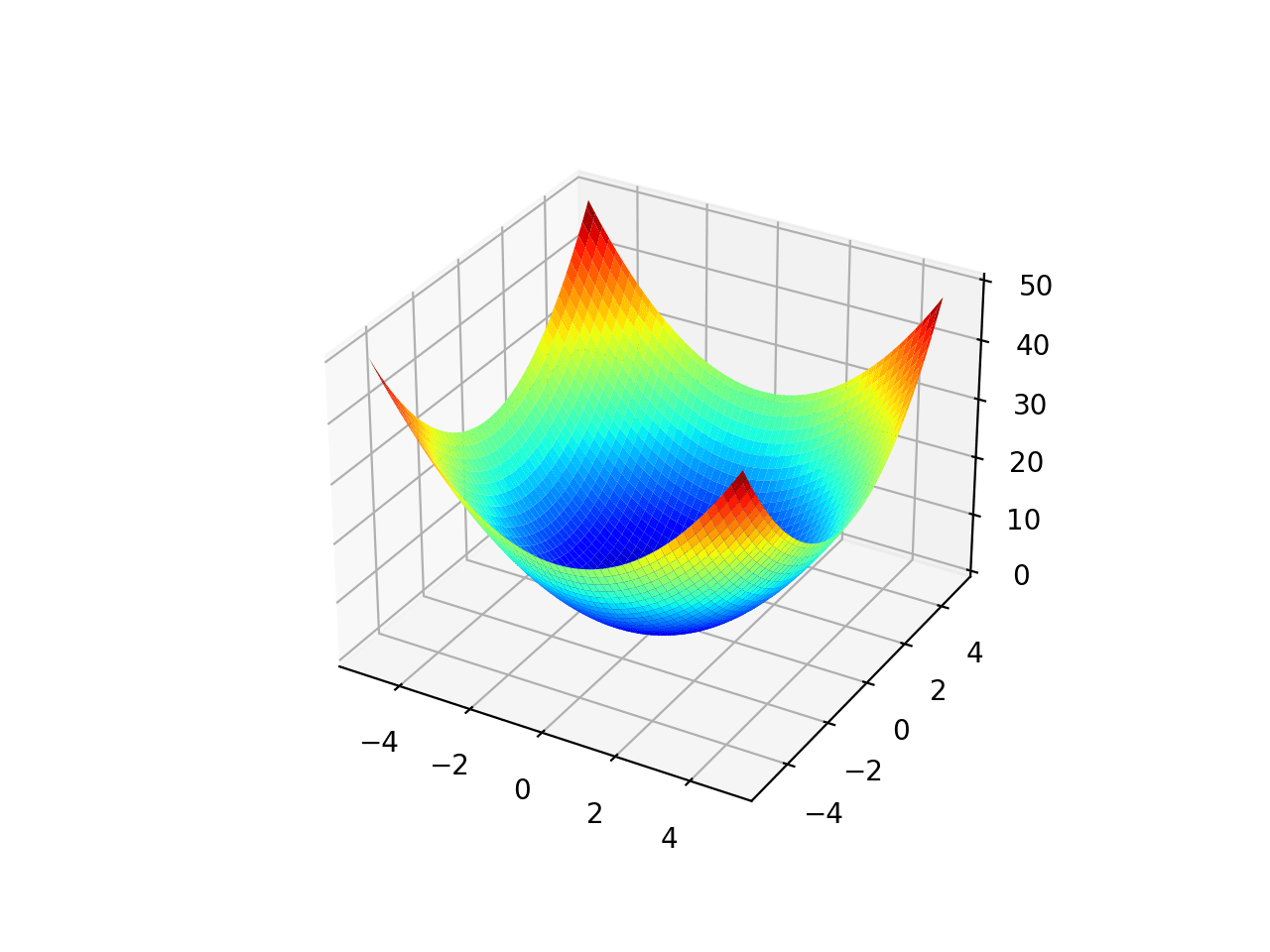
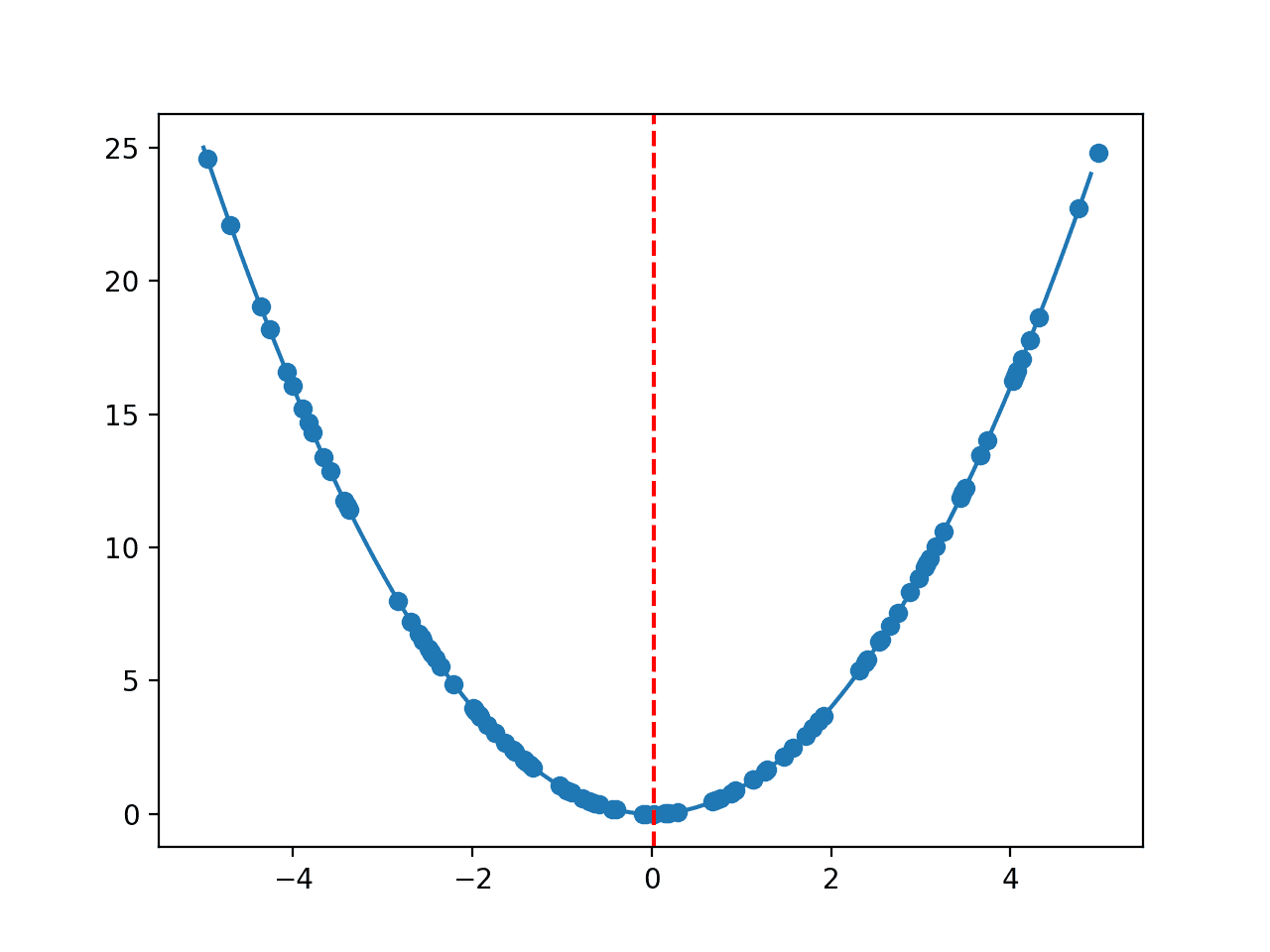
The example below demonstrates how to solve a two-dimensional convex function using the L-BFGS-B local search algorithm.
|
1 2 3 4 5 6 7 8 9 10 11 12 13 14 15 16 17 18 19 20 21 |
# l-bfgs-b algorithm local optimization of a convex function from scipy.optimize import minimize from numpy.random import rand # objective function def objective(x): return x[0]**2.0 + x[1]**2.0 # define range for input r_min, r_max = -5.0, 5.0 # define the starting point as a random sample from the domain pt = r_min + rand(2) * (r_max - r_min) # perform the l-bfgs-b algorithm search result = minimize(objective, pt, method='L-BFGS-B') # summarize the result print('Status : %s' % result['message']) print('Total Evaluations: %d' % result['nfev']) # evaluate solution solution = result['x'] evaluation = objective(solution) print('Solution: f(%s) = %.5f' % (solution, evaluation)) |
Running the example performs the optimization and reports the success or failure of the search, the number of function evaluations performed, and the input that resulted in the optima of the function.
|
1 2 3 |
Status : b'CONVERGENCE: NORM_OF_PROJECTED_GRADIENT_<=_PGTOL' Total Evaluations: 9 Solution: f([3.38059583e-07 3.70089258e-07]) = 0.00000 |
Now that we are familiar with using a local search algorithm with SciPy, let’s look at global search.
Global Search With SciPy
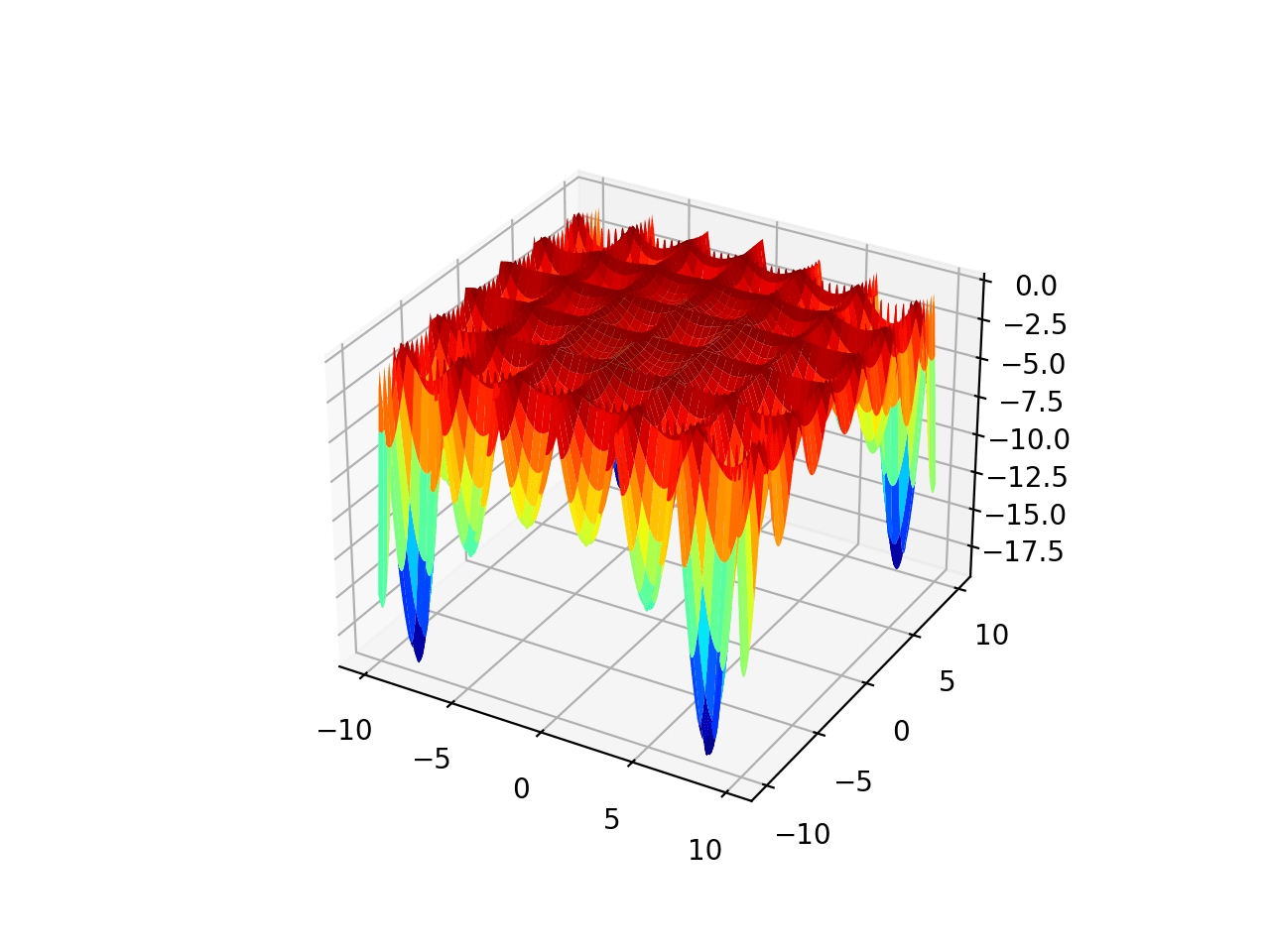
Global search or global function optimization refers to algorithms that seek the input to a function that results in the minimum or maximum output where the function or constrained region being searched is assumed to have multiple local optima, e.g. multimodal.
The function that is being optimized is typically nonlinear, nonconvex, and may have one or more than one input variable.
Global search algorithms are typically stochastic, meaning that they make use of randomness in the search process and may or may not manage a population of candidate solutions as part of the search.
The SciPy library provides a number of stochastic global optimization algorithms, each via different functions. They are:
- Basin Hopping Optimization via the basinhopping() function.
- Differential Evolution Optimization via the differential_evolution() function.
- Simulated Annealing via the dual_annealing() function.
The library also provides the shgo() function for sequence optimization and the brute() for grid search optimization.
Each algorithm returns an OptimizeResult object that summarizes the success or failure of the search and the details of the solution if found.
The example below demonstrates how to solve a two-dimensional multimodal function using simulated annealing.
|
1 2 3 4 5 6 7 8 9 10 11 12 13 14 15 16 17 18 19 20 21 |
# simulated annealing global optimization for a multimodal objective function from scipy.optimize import dual_annealing # objective function def objective(v): x, y = v return (x**2 + y - 11)**2 + (x + y**2 -7)**2 # define range for input r_min, r_max = -5.0, 5.0 # define the bounds on the search bounds = [[r_min, r_max], [r_min, r_max]] # perform the simulated annealing search result = dual_annealing(objective, bounds) # summarize the result print('Status : %s' % result['message']) print('Total Evaluations: %d' % result['nfev']) # evaluate solution solution = result['x'] evaluation = objective(solution) print('Solution: f(%s) = %.5f' % (solution, evaluation)) |
Running the example performs the optimization and reports the success or failure of the search, the number of function evaluations performed, and the input that resulted in the optima of the function.
|
1 2 3 |
Status : ['Maximum number of iteration reached'] Total Evaluations: 4028 Solution: f([-3.77931027 -3.283186 ]) = 0.00000 |
Further Reading
This section provides more resources on the topic if you are looking to go deeper.
APIs
Articles
Summary
In this tutorial, you discovered optimization algorithms provided by the SciPy library.
Specifically, you learned:
- The SciPy library provides a suite of different optimization algorithms for different purposes.
- The local search optimization algorithms available in SciPy.
- The global search optimization algorithms available in SciPy.
Do you have any questions?
Ask your questions in the comments below and I will do my best to answer.


You don’t even know how happy I am you are making this optimization module.
Thank you for your impact!
You’re very welcome!
It’s pretty awesome
Thanks!
Respected , sir good morning
This article is superb .And
I would like to do Ph.D related to this field , can you guide me, now I am persuing Post graduate program in machine learning and artificial intelligence.
Objective : to find chemical level of fruits and vegetables . Because here, in my country nowadays there are using lots of chemicals to grow the plants. So, if we find the chemical level of fruits and vegetables, it is help us to avoid that food to eat . And give awareness of that eagerness of that chemical to the people .
So please can you guide me?
Thanks.
That sounds like a great project.
Sorry, I don’t have the capacity to be your research advisor – I recommend discussing your project with your research group/advisor at your university.
These are awesome details, Jason. I will investigate thoroughly and get back to you.
Thanks!
Hi
I am trying to solve a project where it is Intended to find optimum incentive for insurance agents to maximise Total revenue from premiums paid by subscribers. The agents efforts in hours is a complex exponential function of incentives given and %increase in probability to pay premius is complex exponential function of agents efforts in hours. The total revenue is summation(for all subscribers) of benchmark probability plus %ibcrease in probability to pay premium multiplied by premium amount minus incentive paid to agents. Can I use optimization algorithm here, if yes how? Can you please help me to solve this?
That sounds like a great project!
Perhaps start by trying to define an evaluation function for candidate solutions – it might be a simulation or complex calculation. If you can define an objective function and evaluate candidate solutions, you’re on the right track, then start trying different hand-crafted solutions and eventually an optimization algorithm.
Thanks alot, It is really helpful!!
do you have any idea about how to use the trained neural model as an objective function to apply optimize.minimize function on it ?
Sure, create a function that uses your model with vector input and prediction value output.
Hi Jason,
Thank you for your awesome work. I am trying to use a NN model to minimize the opex of an LNG plant. Can you give an example of how a NN model can be used within the scipy.optimize package?
Thanks in anticipation of your response.
Not sure I understand it but scipy.optimize is to find the minimum of a user-defined function. Hence you want to define a function that take parameters as input, then in the function, you build a NN model using the parameter, do the training, and use the model to produce some value (e.g., error metric). Then this function can be optimized using scipy.
Jason, any link or blog where I can check the working of scipy optimizers from scratch?
Not off hand, sorry.