Curve fitting is a type of optimization that finds an optimal set of parameters for a defined function that best fits a given set of observations.
Unlike supervised learning, curve fitting requires that you define the function that maps examples of inputs to outputs.
The mapping function, also called the basis function can have any form you like, including a straight line (linear regression), a curved line (polynomial regression), and much more. This provides the flexibility and control to define the form of the curve, where an optimization process is used to find the specific optimal parameters of the function.
In this tutorial, you will discover how to perform curve fitting in Python.
After completing this tutorial, you will know:
Curve fitting involves finding the optimal parameters to a function that maps examples of inputs to outputs.
The SciPy Python library provides an API to fit a curve to a dataset.
How to use curve fitting in SciPy to fit a range of different curves to a set of observations.
Kick-start your project with my new book Optimization for Machine Learning, including step-by-step tutorials and the Python source code files for all examples.
Let’s get started.
Curve Fitting With Python Photo by Gael Varoquaux, some rights reserved.
Tutorial Overview
This tutorial is divided into three parts; they are:
Curve Fitting
Curve Fitting Python API
Curve Fitting Worked Example
Curve Fitting
Curve fitting is an optimization problem that finds a line that best fits a collection of observations.
It is easiest to think about curve fitting in two dimensions, such as a graph.
Consider that we have collected examples of data from the problem domain with inputs and outputs.
The x-axis is the independent variable or the input to the function. The y-axis is the dependent variable or the output of the function. We don’t know the form of the function that maps examples of inputs to outputs, but we suspect that we can approximate the function with a standard function form.
Curve fitting involves first defining the functional form of the mapping function (also called the basis function or objective function), then searching for the parameters to the function that result in the minimum error.
Error is calculated by using the observations from the domain and passing the inputs to our candidate mapping function and calculating the output, then comparing the calculated output to the observed output.
Once fit, we can use the mapping function to interpolate or extrapolate new points in the domain. It is common to run a sequence of input values through the mapping function to calculate a sequence of outputs, then create a line plot of the result to show how output varies with input and how well the line fits the observed points.
The key to curve fitting is the form of the mapping function.
A straight line between inputs and outputs can be defined as follows:
y = a * x + b
Where y is the calculated output, x is the input, and a and b are parameters of the mapping function found using an optimization algorithm.
This is called a linear equation because it is a weighted sum of the inputs.
In a linear regression model, these parameters are referred to as coefficients; in a neural network, they are referred to as weights.
This equation can be generalized to any number of inputs, meaning that the notion of curve fitting is not limited to two-dimensions (one input and one output), but could have many input variables.
For example, a line mapping function for two input variables may look as follows:
y = a1 * x1 + a2 * x2 + b
The equation does not have to be a straight line.
We can add curves in the mapping function by adding exponents. For example, we can add a squared version of the input weighted by another parameter:
y = a * x + b * x^2 + c
This is called polynomial regression, and the squared term means it is a second-degree polynomial.
So far, linear equations of this type can be fit by minimizing least squares and can be calculated analytically. This means we can find the optimal values of the parameters using a little linear algebra.
We might also want to add other mathematical functions to the equation, such as sine, cosine, and more. Each term is weighted with a parameter and added to the whole to give the output; for example:
y = a * sin(b * x) + c
Adding arbitrary mathematical functions to our mapping function generally means we cannot calculate the parameters analytically, and instead, we will need to use an iterative optimization algorithm.
This is called nonlinear least squares, as the objective function is no longer convex (it’s nonlinear) and not as easy to solve.
Now that we are familiar with curve fitting, let’s look at how we might perform curve fitting in Python.
Want to Get Started With Optimization Algorithms?
Take my free 7-day email crash course now (with sample code).
Click to sign-up and also get a free PDF Ebook version of the course.
Curve Fitting Python API
We can perform curve fitting for our dataset in Python.
The SciPy open source library provides the curve_fit() function for curve fitting via nonlinear least squares.
The function takes the same input and output data as arguments, as well as the name of the mapping function to use.
The mapping function must take examples of input data and some number of arguments. These remaining arguments will be the coefficients or weight constants that will be optimized by a nonlinear least squares optimization process.
For example, we may have some observations from our domain loaded as input variables x and output variables y.
1
2
3
4
...
# load input variables from a file
x_values=...
y_values=...
Next, we need to design a mapping function to fit a line to the data and implement it as a Python function that takes inputs and the arguments.
It may be a straight line, in which case it would look as follows:
1
2
3
# objective function
def objective(x,a,b,c):
returna *x+b
We can then call the curve_fit() function to fit a straight line to the dataset using our defined function.
The function curve_fit() returns the optimal values for the mapping function, e.g, the coefficient values. It also returns a covariance matrix for the estimated parameters, but we can ignore that for now.
1
2
3
...
# fit curve
popt,_=curve_fit(objective,x_values,y_values)
Once fit, we can use the optimal parameters and our mapping function objective() to calculate the output for any arbitrary input.
This might include the output for the examples we have already collected from the domain, it might include new values that interpolate observed values, or it might include extrapolated values outside of the limits of what was observed.
1
2
3
4
5
6
7
...
# define new input values
x_new=...
# unpack optima parameters for the objective function
a,b,c=popt
# use optimal parameters to calculate new values
y_new=objective(x_new,a,b,c)
Now that we are familiar with using the curve fitting API, let’s look at a worked example.
Curve Fitting Worked Example
We will develop a curve to fit some real world observations of economic data.
In this example, we will use the so-called “Longley’s Economic Regression” dataset; you can learn more about it here:
We will download the dataset automatically as part of the worked example.
There are seven input variables and 16 rows of data, where each row defines a summary of economic details for a year between 1947 to 1962.
In this example, we will explore fitting a line between population size and the number of people employed for each year.
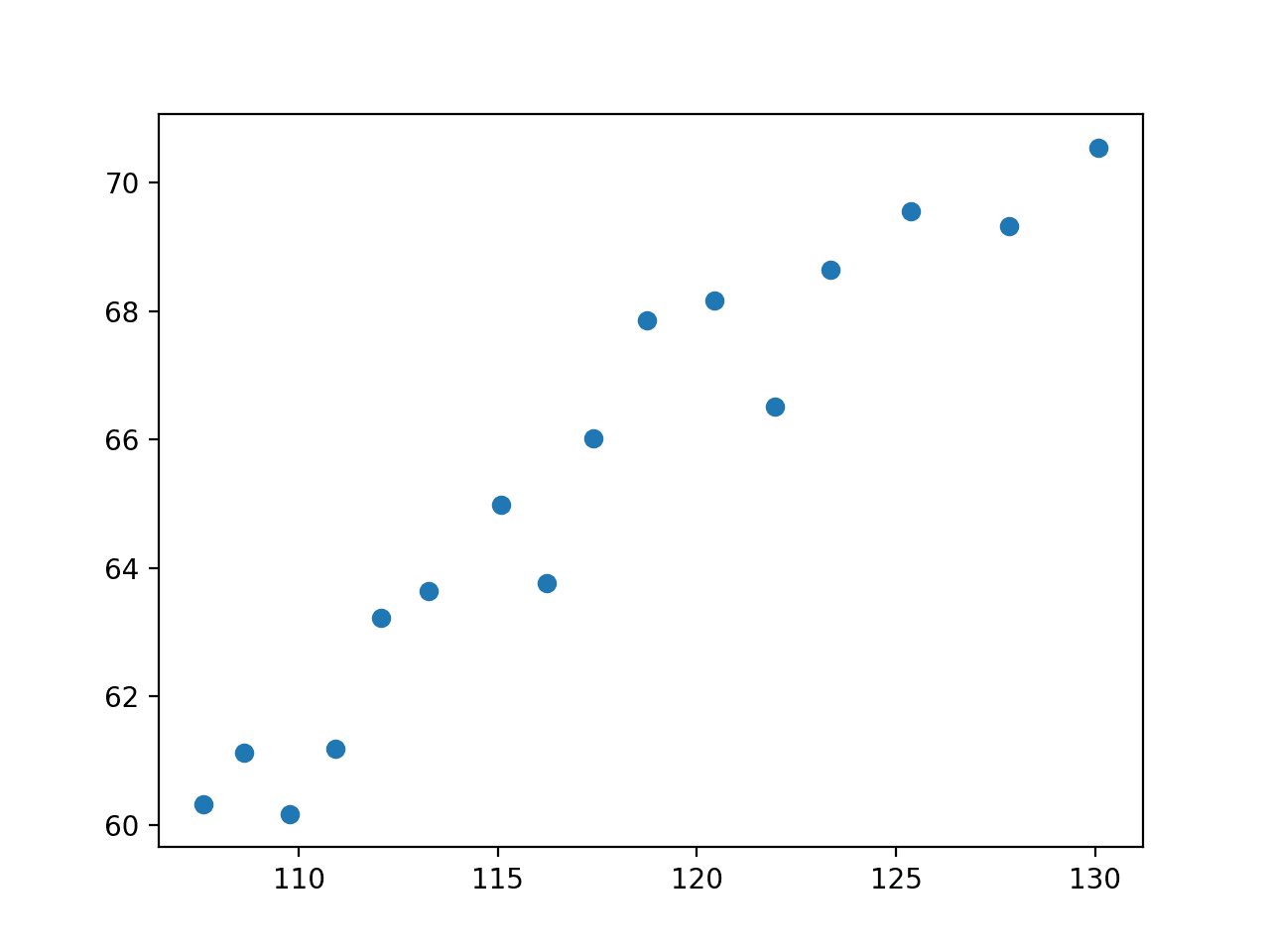
The example below loads the dataset from the URL, selects the input variable as “population,” and the output variable as “employed” and creates a scatter plot.
Running the example loads the dataset, selects the variables, and creates a scatter plot.
We can see that there is a relationship between the two variables. Specifically, that as the population increases, the total number of employees increases.
It is not unreasonable to think we can fit a line to this data.
Scatter Plot of Population vs. Total Employed
First, we will try fitting a straight line to this data, as follows:
1
2
3
# define the true objective function
def objective(x,a,b):
returna *x+b
We can use curve fitting to find the optimal values of “a” and “b” and summarize the values that were found:
1
2
3
4
5
6
...
# curve fit
popt,_=curve_fit(objective,x,y)
# summarize the parameter values
a,b=popt
print('y = %.5f * x + %.5f'%(a,b))
We can then create a scatter plot as before.
1
2
3
...
# plot input vs output
pyplot.scatter(x,y)
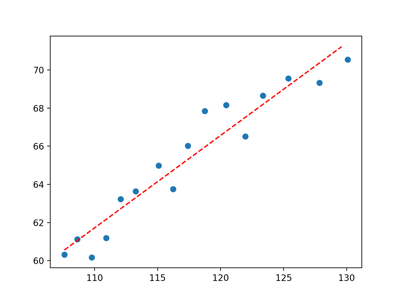
On top of the scatter plot, we can draw a line for the function with the optimized parameter values.
This involves first defining a sequence of input values between the minimum and maximum values observed in the dataset (e.g. between about 120 and about 130).
1
2
3
...
# define a sequence of inputs between the smallest and largest known inputs
x_line=arange(min(x),max(x),1)
We can then calculate the output value for each input value.
1
2
3
...
# calculate the output for the range
y_line=objective(x_line,a,b)
Then create a line plot of the inputs vs. the outputs to see a line:
1
2
3
...
# create a line plot for the mapping function
pyplot.plot(x_line,y_line,'--',color='red')
Tying this together, the example below uses curve fitting to find the parameters of a straight line for our economic data.
# define a sequence of inputs between the smallest and largest known inputs
x_line=arange(min(x),max(x),1)
# calculate the output for the range
y_line=objective(x_line,a,b,c)
# create a line plot for the mapping function
pyplot.plot(x_line,y_line,'--',color='red')
pyplot.show()
First the optimal parameters are reported.
1
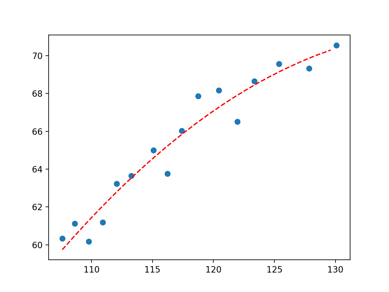
y = 3.25443 * x + -0.01170 * x^2 + -155.02783
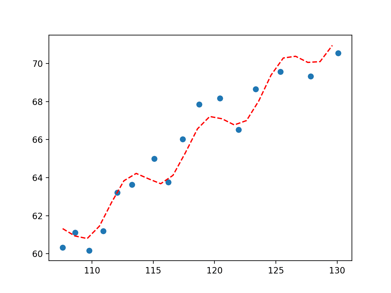
Next, a plot is created showing the line in the context of the observed values from the domain.
We can see that the second-degree polynomial equation that we defined is visually a better fit for the data than the straight line that we tested first.
Plot of Second Degree Polynomial Fit to Economic Dataset
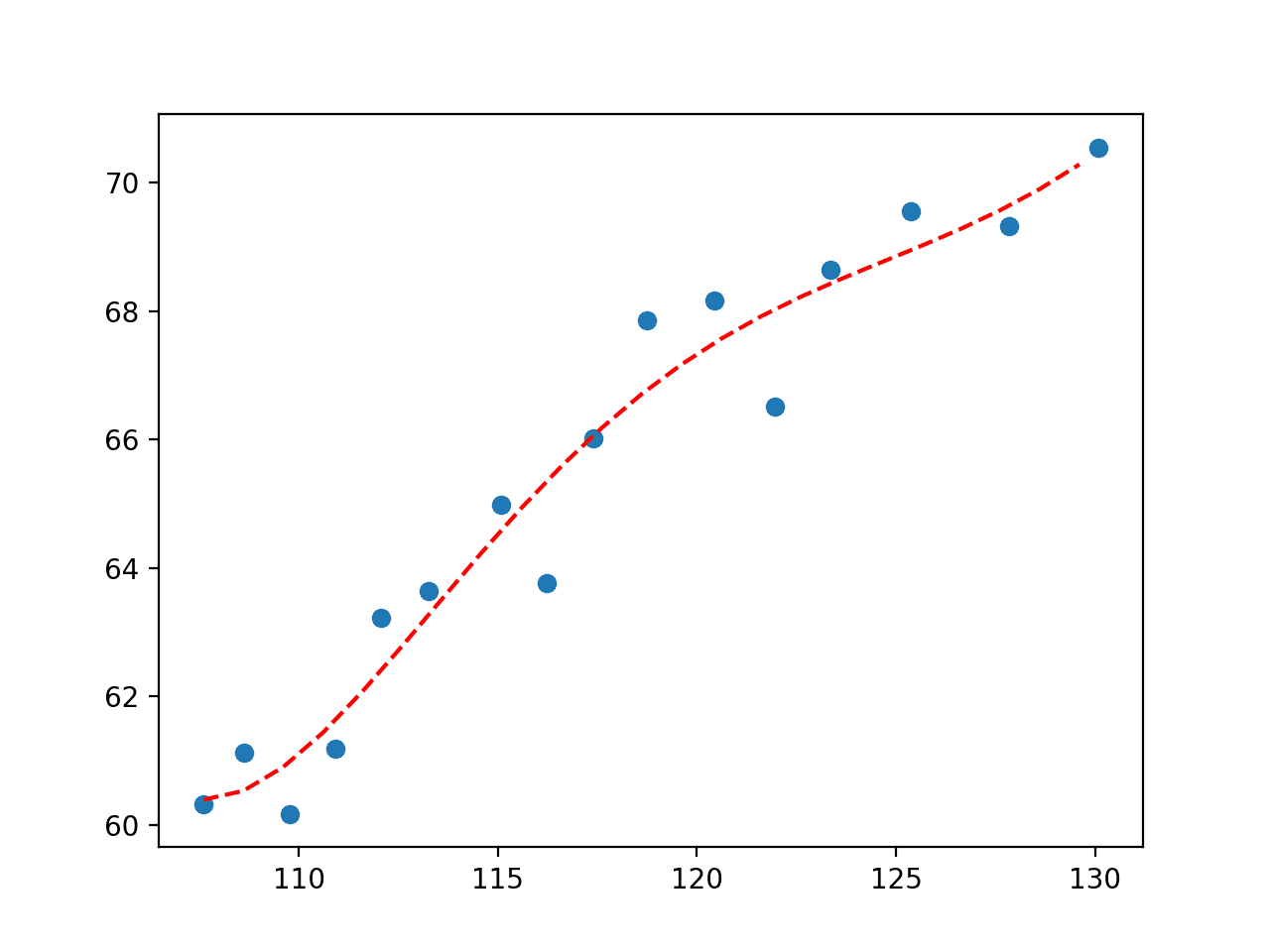
We could keep going and add more polynomial terms to the equation to better fit the curve.
For example, below is an example of a fifth-degree polynomial fit to the data.
1
2
3
4
5
6
7
8
9
10
11
12
13
14
15
16
17
18
19
20
21
22
23
24
25
26
27
28
29
# fit a fifth degree polynomial to the economic data
# define a sequence of inputs between the smallest and largest known inputs
x_line=arange(min(x),max(x),1)
# calculate the output for the range
y_line=objective(x_line,a,b,c,d,e,f)
# create a line plot for the mapping function
pyplot.plot(x_line,y_line,'--',color='red')
pyplot.show()
Running the example fits the curve and plots the result, again capturing slightly more nuance in how the relationship in the data changes over time.
Plot of Fifth Degree Polynomial Fit to Economic Dataset
Importantly, we are not limited to linear regression or polynomial regression. We can use any arbitrary basis function.
For example, perhaps we want a line that has wiggles to capture the short-term movement in observation. We could add a sine curve to the equation and find the parameters that best integrate this element in the equation.
For example, an arbitrary function that uses a sine wave and a second degree polynomial is listed below:
1
2
3
# define the true objective function
def objective(x,a,b,c,d):
returna *sin(b-x)+c *x**2+d
The complete example of fitting a curve using this basis function is listed below.
# define a sequence of inputs between the smallest and largest known inputs
x_line=arange(min(x),max(x),1)
# calculate the output for the range
y_line=objective(x_line,a,b,c,d)
# create a line plot for the mapping function
pyplot.plot(x_line,y_line,'--',color='red')
pyplot.show()
Running the example fits a curve and plots the result.
We can see that adding a sine wave has the desired effect showing a periodic wiggle with an upward trend that provides another way of capturing the relationships in the data.
Plot of Sine Wave Fit to Economic Dataset
How do you choose the best fit?
If you want the best fit, you would model the problem as a regression supervised learning problem and test a suite of algorithms in order to discover which is best at minimizing the error.
In this case, curve fitting is appropriate when you want to define the function explicitly, then discover the parameters of your function that best fit a line to the data.
Further Reading
This section provides more resources on the topic if you are looking to go deeper.
It provides self-study tutorials with full working code on: Gradient Descent, Genetic Algorithms, Hill Climbing, Curve Fitting, RMSProp, Adam,
and much more...
Bring Modern Optimization Algorithms to Your Machine Learning Projects
Thanks for the article! Do you have any good links or tutorials for adding constraints? For example, I am trying to fit the sum of several Gaussians to a set of data. I am playing with adding constraints on:
– the area of each Gaussian
– the center of each Gaussian
– The relative areas of different Gaussians
– etc.
I have been using a penalty method to apply the constraints. Trial and error (playing with the penalty factors) has allowed me to achieve believable results, but I’m wondering if there is a systematic way to find good penalty factors as more constraints are added. The solution becomes a bit unstable as I add more constraints (small changes in penalty factor result in different fits).
I’ve modified your code to read the CSV data file from my local machine. I saved the CSV file and made these changes; but somehow I didn’t get what I want.
This is great information. One question I have is how to accomplish curve fitting for multiple samples. Say for example we have data points for four independent runs of an experiment representing user 1 – user 4. Ideally I’d like to take these 4 runs and create a curve that “fits” all four runs and presents one equation that is optimal. I’m not clear how to accomplish this with python’s curve fitting function. Can you clarify how this would be accomplished
Not really sure I follow – let me try – if you want a curve that generalizes across 4 samples of the population, perhaps combine the 4 samples into one sample and fit a curve to that?
Hi, Jason. Thanks for the really useful post.
I have a stupid question because I am a newbie in Python.
In your example you typed,
# choose the input and output variables
x, y = data[:, 4], data[:, -1]
Why is x=data[:,4] and y=data[:,-1]?
In the dataset in .csv, Population seems in the 5th column and Total Employed in the last column. Then, how the column indices for x and y are corresponding to 4 and -1?
Hi, I have a problem I’m trying to run some analysis on my data using LRP (Linear Response Plateau) but I’m pretty lost with the broken-line equation and how to insert it into python. Can you help?
Hi Jason,
Thanks for sharing the important information.
I have experimental data consisting of inputs and corresponding outputs. I want to find the best model fitting the data. As you said in the last paragraph, use “a regression supervised learning problem.” Can you please elaborate more on this, or can you please give an example with the source code?
Very nice post. Had a doubt, is it possible to do curve fitting on 3 feature together with 1 target variable ? Like temp, humidity and windspeed with target variable PlantFungusGrowth.
Please help. Thanks
If all are floating point values, of course you can. Simply define your objective function (e.g., growth depends on temp or square of temp?) and call curve_fit()
If my best fit equation looks like below. Does this means that coefficient of x^2 and x^3 is 0 or it is very small that can not fit in 5 decimal digits? If it is later how can I get the non-zero value of the x^2 and x^3 coefficients?
y = -0.00839 * x + 0.00000 * x^2 + -0.00000 * x^3 + 5.10433
It depends on your data. If your x is large, x^2 and x^3 may be even larger and hence it shows zero. In this case, you may still find the coefficient in higher precision by printing “%.9f” instead of “%.5f”. If your x is not large, it simply means the curve fitting suggest you to use linear instead of degree-3 curve.
Great tutorial! I wonder if how to define a model for curve fitting if the model is calculated in time series ( the calculated result is based on previous result)?
Not exactly understood what you’re asking but think in this way: If you can mentally tell your model is y=f(x) and know what are x and y, then you can fit a curve on it.
Curve fitting is probably not the entire step here. You may consider ∆y(t) = y(t)-y(t-1) and rearrange your equation into ∆y(t) = a + bx(t); then you do a curve fitting on this. Afterwards, you can do integration to get back y(t) in terms of x(t)
Very helpful post! I’m using this fit model to fit microbial growth curves and I’m struggling with finding Y giving X. Any tips? I’m sure is easy to solve but I’m new to coding
Purchased some of your materials years ago – great stuff!
Now I am back and this is an excellent from-the-ground-up explanation.
Question: do you have a blog post or other material on this last statement –
“If you want the best fit, you would model the problem as a regression supervised learning problem and test a suite of algorithms in order to discover which is best at minimizing the error.”
This was incredibly useful – I have bookmarked this page as I’m sure I’ll have to solve problems like this again. I needed to fit x/y valuest to a line in order to determine x for new values. This was exactly what I needed!
Thank you
I’m a bit lost with my curve fitting problem and would appreciate a little help 🙂
I am trying to fit a curve like a * exp(b * x + c) + d with 13 data points (observations). I am doing exactly as described here but for some reason, the “solution” parameters basically leave me with a straight line (for the range of the observations). Would love to share the graph but this does not seem to be possible here in the comments section.
Has anyone experienced anything like that and has an advice for me?
Thanks so much for any hint on that!
Best, N
Hi. My problem is a little bit different. I have some curves that changes with parameter like A. for example I have a curve for A1 and a different curve for A2. if parameter A1<A<A2, how can i have the curve for A?
Hi, I’m getting a ” ‘Series’ object is not callable ” error when using your arbitrary function code, and it seems like the problem is coming from this line in my code:
x, y = data3[“Vertices”], data3[“Avg Comparisons”]
Where data3 is a Dataframe. Any idea why this is happening?
Thank you so much for posting this. Ques: The curve_fit function returns the covariances between the parameters (coefficients for x and the intercept, etc) If there is a high covariance between the parameters what does this tell us? Is this bad? If so why? thankx!
In this example:
# define the true objective function
def objective(x, a, b, c, d):
return a * sin(b – x) + c * x**2 + d
.
.
.
popt, _ = curve_fit(objective, x, y)
I get this error “Improper input: func input vector length N=4 must not exceed func output vector length M=2” can you please help me fix this?
Hello…The error message you’re encountering, “Improper input: func input vector length N=4 must not exceed func output vector length M=2,” is typically associated with the use of the curve_fit function from the scipy.optimize module. This error suggests that there’s a mismatch between the number of parameters your function is expecting and the dimensions or shape of the data being passed to it.
In the context of the curve_fit function, the objective function should be defined in a way that it takes the independent variable (x) as the first argument and all the parameters to be optimized as subsequent arguments. It should then return the dependent variable (y). Let’s revisit your function:
python

from numpy import sin
# Define the true objective function
def objective(x, a, b, c, d):
return a * sin(b - x) + c * x**2 + d
Given this definition, the function objective expects five arguments: x, a, b, c, and d. Here’s a breakdown of how to use it with curve_fit:
1. Ensure your x and y data are correctly formatted as arrays.
2. Provide initial guesses for the parameters a, b, c, and d.
Here’s a complete example including dummy data and the curve fitting process:
python

import numpy as np

from scipy.optimize import curve_fit

from numpy import sin
# Define the objective function
def objective(x, a, b, c, d):
return a * sin(b - x) + c * x**2 + d
# Create dummy data
x_data = np.linspace(0, 4, 50) # 50 points from 0 to 4
y_data = objective(x_data, 2.5, 1.3, 0.5, 1.0) + 0.2 * np.random.normal(size=x_data.size) # Add some noise
# Initial guesses for a, b, c, d
initial_guess = [1.0, 1.0, 1.0, 1.0]
# Print the optimized parameters
print("Optimized Parameters:", popt)
This script performs the following:
– Defines the objective function as required.
– Generates some dummy x data and corresponding y data using the objective function with some noise added.
– Provides initial guesses for the parameters [a, b, c, d].
– Uses curve_fit to optimize the parameters based on the data.
Ensure that your x and y data are of compatible sizes and correctly formatted as numpy arrays. If your data or setup differs significantly, you may need to adjust the example accordingly. If you’re still having trouble, ensure the data dimensions and types are correctly set up for curve_fit to process.


Great Jason!!
As always, very useful.
Thanks for you work.
Thanks!
Dear Jason Brownlee,
thank you for this great post.
I wonder if you could further elaborate how one may interpret and analyze the covariance matrix from the fitting function.
I thank you for your time.
Sincerely,
Thanks!
Great suggestion.
Fantastic post! Thank you
Thank you!
Great tutorial I’ve done it succesfully!
Only thing I needed to do differently is import numpy and scipy to get it working.
Question: How can I measure or calculate the error of the curve to the real data?
You can calculate the error between expected and predicted values, typically MAE or RMSE.
Thanks for share this information. It is very valuable. Some friend recommend your material.
I would like to know , if you have your lesson and practices problem in YouTube?
Please comment about your method and course online course of ML
You’re welcome.
Sorry, I don’t have any youtube videos.
I offer self-study ebook courses here:
https://machinelearningmastery.com/products/
Thanks for the article! Do you have any good links or tutorials for adding constraints? For example, I am trying to fit the sum of several Gaussians to a set of data. I am playing with adding constraints on:
– the area of each Gaussian
– the center of each Gaussian
– The relative areas of different Gaussians
– etc.
I have been using a penalty method to apply the constraints. Trial and error (playing with the penalty factors) has allowed me to achieve believable results, but I’m wondering if there is a systematic way to find good penalty factors as more constraints are added. The solution becomes a bit unstable as I add more constraints (small changes in penalty factor result in different fits).
Interesting project. Sorry, I don’t have good comments off the cuff. Perhaps check a text on multivariate analysis or multivariate stats?
Thank you for the good sharing!
I’ve modified your code to read the CSV data file from my local machine. I saved the CSV file and made these changes; but somehow I didn’t get what I want.
import pandas as pd
data = pd.read_csv(‘data.csv’, delimiter=’,’)
Perhaps this will help:
https://machinelearningmastery.com/load-machine-learning-data-python/
This is great information. One question I have is how to accomplish curve fitting for multiple samples. Say for example we have data points for four independent runs of an experiment representing user 1 – user 4. Ideally I’d like to take these 4 runs and create a curve that “fits” all four runs and presents one equation that is optimal. I’m not clear how to accomplish this with python’s curve fitting function. Can you clarify how this would be accomplished
Thanks.
Not really sure I follow – let me try – if you want a curve that generalizes across 4 samples of the population, perhaps combine the 4 samples into one sample and fit a curve to that?
Does that help?
Thanks, you helped me a lot with this post.
You’re welcome.
What python package do you recommend for assessing the best fit?
Often we use an error metric, like R^2 or MSE.
Hi, Jason. Thanks for the really useful post.
I have a stupid question because I am a newbie in Python.
In your example you typed,
# choose the input and output variables
x, y = data[:, 4], data[:, -1]
Why is x=data[:,4] and y=data[:,-1]?
In the dataset in .csv, Population seems in the 5th column and Total Employed in the last column. Then, how the column indices for x and y are corresponding to 4 and -1?
Thanks again.
Good question, if you are new to python array indexes, this will help:
https://machinelearningmastery.com/index-slice-reshape-numpy-arrays-machine-learning-python/
Wow, so much flexibility..
Thanks for the quick reply!
You’re welcome.
Man, this is the best article about curve fitting I have came across. Thanks alot.
Thanks!
I have to do a Blackbody fit. The function is
def bb(x, T):
from scipy.constants import h,k,c
x = 1e-6 * x # convert to metres from um
return 2*h*c**2 / (x**5 * (np.exp(h*c / (x*k*T)) – 1))
How do I take care of the input for the Temperature T?
thanks in advance
R. Baer
I don’t know sorry.
Hi, I have a problem I’m trying to run some analysis on my data using LRP (Linear Response Plateau) but I’m pretty lost with the broken-line equation and how to insert it into python. Can you help?
Sorry, I am not familiar with “LRP” off the cuff.
Great tutorial! I am running into an error however:
from scipy.optimize import curve_fit
def objective (qi,a,b):
return qi*n + b
chargedata = loadtxt(“242E1charges.tsv”, float, skiprows = 1)
qi = chargedata[:,:]
n = qi//qs
plot(qi,n, “rd”, label =”data points”)
fit, _ = curve_fit(objective, qi, n)
where I am using qi alternatively to x.
the error that pops up is:
Result from function call is not a proper array of floats.
any ideas on how to fix this? I am somewhat new to python so I apologize if the solution is elementary.
No sorry, this looks like custom code.
Perhaps you can post your code, data and error on stackoverflow.com
Hi, Any idea on how we can do curve fitting on a time series?
Your tutorials are of great help,Thankyou!
Not off hand, perhaps the same methods can be adapted.
Hi!
how can we predict using curve fitting?
Curve fitting is not for prediction, perhaps you want to use time series forecasting methods:
https://machinelearningmastery.com/start-here/#timeseries
Hi Jason,
Thanks for sharing the important information.
I have experimental data consisting of inputs and corresponding outputs. I want to find the best model fitting the data. As you said in the last paragraph, use “a regression supervised learning problem.” Can you please elaborate more on this, or can you please give an example with the source code?
Perhaps this will help:
https://machinelearningmastery.com/?s=regression&post_type=post&submit=Search
Can we do 2D array [x,y] curve fitting where x and y are not monotonic?
Perhaps try it and see.
Thanks, you made it so simple for us!
You’re welcome!
Thank you for this great post. Helped me a lot.
I’m happy to hear that.
Very nice post. Had a doubt, is it possible to do curve fitting on 3 feature together with 1 target variable ? Like temp, humidity and windspeed with target variable PlantFungusGrowth.
Please help. Thanks
If all are floating point values, of course you can. Simply define your objective function (e.g., growth depends on temp or square of temp?) and call curve_fit()
Hi thank you for the great post.
If my best fit equation looks like below. Does this means that coefficient of x^2 and x^3 is 0 or it is very small that can not fit in 5 decimal digits? If it is later how can I get the non-zero value of the x^2 and x^3 coefficients?
y = -0.00839 * x + 0.00000 * x^2 + -0.00000 * x^3 + 5.10433
Thank you in advance.
It depends on your data. If your x is large, x^2 and x^3 may be even larger and hence it shows zero. In this case, you may still find the coefficient in higher precision by printing “%.9f” instead of “%.5f”. If your x is not large, it simply means the curve fitting suggest you to use linear instead of degree-3 curve.
Great tutorial! I wonder if how to define a model for curve fitting if the model is calculated in time series ( the calculated result is based on previous result)?
Not exactly understood what you’re asking but think in this way: If you can mentally tell your model is y=f(x) and know what are x and y, then you can fit a curve on it.
I mean if my model is y(t) = y(t-1) + a + bx(t) where t is index. how do we define it in equation of curve fit?
Curve fitting is probably not the entire step here. You may consider ∆y(t) = y(t)-y(t-1) and rearrange your equation into ∆y(t) = a + bx(t); then you do a curve fitting on this. Afterwards, you can do integration to get back y(t) in terms of x(t)
Wonderful. Thank you so much.
You are very welcome Jithesh!
Very helpful post! I’m using this fit model to fit microbial growth curves and I’m struggling with finding Y giving X. Any tips? I’m sure is easy to solve but I’m new to coding
Hi Mairana…The following may be a great starting point for someone new to programming:
https://machinelearningmastery.com/regression-machine-learning-tutorial-weka/
Hi Jason,
Purchased some of your materials years ago – great stuff!
Now I am back and this is an excellent from-the-ground-up explanation.
Question: do you have a blog post or other material on this last statement –
“If you want the best fit, you would model the problem as a regression supervised learning problem and test a suite of algorithms in order to discover which is best at minimizing the error.”
Thanks!
Hi Kevin…The following resources may be of interest:
https://machinelearningmastery.com/regression-tutorial-keras-deep-learning-library-python/
https://machinelearningmastery.com/linear-regression-tutorial-using-gradient-descent-for-machine-learning/
https://machinelearningmastery.com/linear-regression-for-machine-learning/
If have any specific goals for your models, we can help clarify additional approaches.
Very helpful page. God job!
Thank you for the feedback EllieM!
This was incredibly useful – I have bookmarked this page as I’m sure I’ll have to solve problems like this again. I needed to fit x/y valuest to a line in order to determine x for new values. This was exactly what I needed!
Thank you
Thank you for the great feedback Mariana!
Dear Jason & community,
I’m a bit lost with my curve fitting problem and would appreciate a little help 🙂
I am trying to fit a curve like a * exp(b * x + c) + d with 13 data points (observations). I am doing exactly as described here but for some reason, the “solution” parameters basically leave me with a straight line (for the range of the observations). Would love to share the graph but this does not seem to be possible here in the comments section.
Has anyone experienced anything like that and has an advice for me?
Thanks so much for any hint on that!
Best, N
Hi Nadja…the following resource has many examples that may prove helpful for you:
https://gekko.readthedocs.io/en/latest/index.html
Hi. My problem is a little bit different. I have some curves that changes with parameter like A. for example I have a curve for A1 and a different curve for A2. if parameter A1<A<A2, how can i have the curve for A?
Hi Mina…The following resource may add clarity:
https://www.kaggle.com/code/residentmario/non-parametric-regression/notebook
Hi, I’m getting a ” ‘Series’ object is not callable ” error when using your arbitrary function code, and it seems like the problem is coming from this line in my code:
x, y = data3[“Vertices”], data3[“Avg Comparisons”]
Where data3 is a Dataframe. Any idea why this is happening?
Hi Wong…Did you copy and paste the code listing or type it? Also, you may want to try the code in Google Colab. Let us know what you find!
Thank you so much for posting this. Ques: The curve_fit function returns the covariances between the parameters (coefficients for x and the intercept, etc) If there is a high covariance between the parameters what does this tell us? Is this bad? If so why? thankx!
Thanks for the post, James. Do you have additional code to solve the RMSE and Rsq values from the fit?
Hi Josh…The following may be of interest:
https://machinelearningmastery.com/regression-metrics-for-machine-learning/
I guess that would include predictive modeling…..
Thanks for the post – Is there a way to get the test statistics + p-values for each of the returned coefficients of the fitted curve?
Hi Christopher…You are very welcome! The following discussion provides some considerations regarding results obtained from regression:
https://stackoverflow.com/questions/27928275/find-p-value-significance-in-scikit-learn-linearregression
In this example:
# define the true objective function
def objective(x, a, b, c, d):
return a * sin(b – x) + c * x**2 + d
.
.
.
popt, _ = curve_fit(objective, x, y)
I get this error “Improper input: func input vector length N=4 must not exceed func output vector length M=2” can you please help me fix this?
Hello…The error message you’re encountering, “Improper input: func input vector length N=4 must not exceed func output vector length M=2,” is typically associated with the use of the
curve_fitfunction from thescipy.optimizemodule. This error suggests that there’s a mismatch between the number of parameters your function is expecting and the dimensions or shape of the data being passed to it.In the context of the
curve_fitfunction, the objective function should be defined in a way that it takes the independent variable (x) as the first argument and all the parameters to be optimized as subsequent arguments. It should then return the dependent variable (y). Let’s revisit your function:pythonfrom numpy import sin
# Define the true objective function
def objective(x, a, b, c, d):
return a * sin(b - x) + c * x**2 + d
Given this definition, the function
objectiveexpects five arguments:x,a,b,c, andd. Here’s a breakdown of how to use it withcurve_fit:1. Ensure your
xandydata are correctly formatted as arrays.2. Provide initial guesses for the parameters
a,b,c, andd.Here’s a complete example including dummy data and the curve fitting process:
pythonimport numpy as np
from scipy.optimize import curve_fit
from numpy import sin
# Define the objective function
def objective(x, a, b, c, d):
return a * sin(b - x) + c * x**2 + d
# Create dummy data
x_data = np.linspace(0, 4, 50) # 50 points from 0 to 4
y_data = objective(x_data, 2.5, 1.3, 0.5, 1.0) + 0.2 * np.random.normal(size=x_data.size) # Add some noise
# Initial guesses for a, b, c, d
initial_guess = [1.0, 1.0, 1.0, 1.0]
# Perform curve fitting
popt, pcov = curve_fit(objective, x_data, y_data, p0=initial_guess)
# Print the optimized parameters
print("Optimized Parameters:", popt)
This script performs the following:
– Defines the objective function as required.
– Generates some dummy
xdata and correspondingydata using the objective function with some noise added.– Provides initial guesses for the parameters
[a, b, c, d].– Uses
curve_fitto optimize the parameters based on the data.Ensure that your
xandydata are of compatible sizes and correctly formatted as numpy arrays. If your data or setup differs significantly, you may need to adjust the example accordingly. If you’re still having trouble, ensure the data dimensions and types are correctly set up forcurve_fitto process.