Random Forest is a popular and effective ensemble machine learning algorithm.
It is widely used for classification and regression predictive modeling problems with structured (tabular) data sets, e.g. data as it looks in a spreadsheet or database table.
Random Forest can also be used for time series forecasting, although it requires that the time series dataset be transformed into a supervised learning problem first. It also requires the use of a specialized technique for evaluating the model called walk-forward validation, as evaluating the model using k-fold cross validation would result in optimistically biased results.
In this tutorial, you will discover how to develop a Random Forest model for time series forecasting.
After completing this tutorial, you will know:
Random Forest is an ensemble of decision trees algorithms that can be used for classification and regression predictive modeling.
Time series datasets can be transformed into supervised learning using a sliding-window representation.
How to fit, evaluate, and make predictions with an Random Forest regression model for time series forecasting.
Let’s get started.
Random Forest for Time Series Forecasting Photo by IvyMike, some rights reserved.
Tutorial Overview
This tutorial is divided into three parts; they are:
Random Forest Ensemble
Time Series Data Preparation
Random Forest for Time Series
Random Forest Ensemble
Random forest is an ensemble of decision tree algorithms.
It is an extension of bootstrap aggregation (bagging) of decision trees and can be used for classification and regression problems.
In bagging, a number of decision trees are made where each tree is created from a different bootstrap sample of the training dataset. A bootstrap sample is a sample of the training dataset where an example may appear more than once in the sample. This is referred to as “sampling with replacement”.
Bagging is an effective ensemble algorithm as each decision tree is fit on a slightly different training dataset, and in turn, has a slightly different performance. Unlike normal decision tree models, such as classification and regression trees (CART), trees used in the ensemble are unpruned, making them slightly overfit to the training dataset. This is desirable as it helps to make each tree more different and have less correlated predictions or prediction errors.
Predictions from the trees are averaged across all decision trees, resulting in better performance than any single tree in the model.
A prediction on a regression problem is the average of the prediction across the trees in the ensemble. A prediction on a classification problem is the majority vote for the class label across the trees in the ensemble.
Regression: Prediction is the average prediction across the decision trees.
Classification: Prediction is the majority vote class label predicted across the decision trees.
Random forest involves constructing a large number of decision trees from bootstrap samples from the training dataset, like bagging.
Unlike bagging, random forest also involves selecting a subset of input features (columns or variables) at each split point in the construction of the trees. Typically, constructing a decision tree involves evaluating the value for each input variable in the data in order to select a split point. By reducing the features to a random subset that may be considered at each split point, it forces each decision tree in the ensemble to be more different.
The effect is that the predictions, and in turn, prediction errors, made by each tree in the ensemble are more different or less correlated. When the predictions from these less correlated trees are averaged to make a prediction, it often results in better performance than bagged decision trees.
For more on the Random Forest algorithm, see the tutorial:
Time series data can be phrased as supervised learning.
Given a sequence of numbers for a time series dataset, we can restructure the data to look like a supervised learning problem. We can do this by using previous time steps as input variables and use the next time step as the output variable.
Let’s make this concrete with an example. Imagine we have a time series as follows:
1
2
3
4
5
6
time, measure
1, 100
2, 110
3, 108
4, 115
5, 120
We can restructure this time series dataset as a supervised learning problem by using the value at the previous time step to predict the value at the next time-step.
Reorganizing the time series dataset this way, the data would look as follows:
1
2
3
4
5
6
7
X, y
?, 100
100, 110
110, 108
108, 115
115, 120
120, ?
Note that the time column is dropped and some rows of data are unusable for training a model, such as the first and the last.
This representation is called a sliding window, as the window of inputs and expected outputs is shifted forward through time to create new “samples” for a supervised learning model.
For more on the sliding window approach to preparing time series forecasting data, see the tutorial:
We can use the shift() function in Pandas to automatically create new framings of time series problems given the desired length of input and output sequences.
This would be a useful tool as it would allow us to explore different framings of a time series problem with machine learning algorithms to see which might result in better-performing models.
The function below will take a time series as a NumPy array time series with one or more columns and transform it into a supervised learning problem with the specified number of inputs and outputs.
1
2
3
4
5
6
7
8
9
10
11
12
13
14
15
16
17
# transform a time series dataset into a supervised learning dataset
Once the dataset is prepared, we must be careful in how it is used to fit and evaluate a model.
For example, it would not be valid to fit the model on data from the future and have it predict the past. The model must be trained on the past and predict the future.
This means that methods that randomize the dataset during evaluation, like k-fold cross-validation, cannot be used. Instead, we must use a technique called walk-forward validation.
In walk-forward validation, the dataset is first split into train and test sets by selecting a cut point, e.g. all data except the last 12 months is used for training and the last 12 months is used for testing.
If we are interested in making a one-step forecast, e.g. one month, then we can evaluate the model by training on the training dataset and predicting the first step in the test dataset. We can then add the real observation from the test set to the training dataset, refit the model, then have the model predict the second step in the test dataset.
Repeating this process for the entire test dataset will give a one-step prediction for the entire test dataset from which an error measure can be calculated to evaluate the skill of the model.
For more on walk-forward validation, see the tutorial:
The function below performs walk-forward validation.
It takes the entire supervised learning version of the time series dataset and the number of rows to use as the test set as arguments.
It then steps through the test set, calling the random_forest_forecast() function to make a one-step forecast. An error measure is calculated and the details are returned for analysis.
1
2
3
4
5
6
7
8
9
10
11
12
13
14
15
16
17
18
19
20
21
22
# walk-forward validation for univariate data
def walk_forward_validation(data,n_test):
predictions=list()
# split dataset
train,test=train_test_split(data,n_test)
# seed history with training dataset
history=[xforxintrain]
# step over each time-step in the test set
foriinrange(len(test)):
# split test row into input and output columns
testX,testy=test[i,:-1],test[i,-1]
# fit model on history and make a prediction
yhat=random_forest_forecast(history,testX)
# store forecast in list of predictions
predictions.append(yhat)
# add actual observation to history for the next loop
The random_forest_forecast() function below implements this, taking the training dataset and test input row as input, fitting a model and making a one-step prediction.
1
2
3
4
5
6
7
8
9
10
11
12
# fit an random forest model and make a one step prediction
def random_forest_forecast(train,testX):
# transform list into array
train=asarray(train)
# split into input and output columns
trainX,trainy=train[:,:-1],train[:,-1]
# fit model
model=RandomForestRegressor(n_estimators=1000)
model.fit(trainX,trainy)
# make a one-step prediction
yhat=model.predict([testX])
returnyhat[0]
Now that we know how to prepare time series data for forecasting and evaluate a Random Forest model, next we can look at using Random Forest on a real dataset.
Random Forest for Time Series
In this section, we will explore how to use the Random Forest regressor for time series forecasting.
We will use a standard univariate time series dataset with the intent of using the model to make a one-step forecast.
You can use the code in this section as the starting point in your own project and easily adapt it for multivariate inputs, multivariate forecasts, and multi-step forecasts.
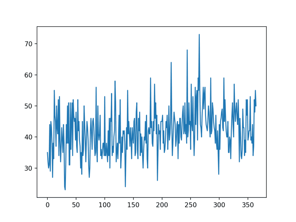
We will use the daily female births dataset, that is the monthly births across three years.
You can download the dataset from here, place it in your current working directory with the filename “daily-total-female-births.csv“.
Running the example creates a line plot of the dataset.
We can see there is no obvious trend or seasonality.
Line Plot of Monthly Births Time Series Dataset
A persistence model can achieve a MAE of about 6.7 births when predicting the last 12 months. This provides a baseline in performance above which a model may be considered skillful.
Next, we can evaluate the Random Forest model on the dataset when making one-step forecasts for the last 12 months of data.
We will use only the previous six time steps as input to the model and default model hyperparameters, except we will use 1,000 trees in the ensemble (to avoid underlearning).
The complete example is listed below.
1
2
3
4
5
6
7
8
9
10
11
12
13
14
15
16
17
18
19
20
21
22
23
24
25
26
27
28
29
30
31
32
33
34
35
36
37
38
39
40
41
42
43
44
45
46
47
48
49
50
51
52
53
54
55
56
57
58
59
60
61
62
63
64
65
66
67
68
69
70
71
72
73
74
75
76
77
78
79
80
# forecast monthly births with random forest
from numpy import asarray
from pandas import read_csv
from pandas import DataFrame
from pandas import concat
from sklearn.metrics import mean_absolute_error
from sklearn.ensemble import RandomForestRegressor
from matplotlib import pyplot
# transform a time series dataset into a supervised learning dataset
# transform the time series data into supervised learning
data=series_to_supervised(values,n_in=6)
# evaluate
mae,y,yhat=walk_forward_validation(data,12)
print('MAE: %.3f'%mae)
# plot expected vs predicted
pyplot.plot(y,label='Expected')
pyplot.plot(yhat,label='Predicted')
pyplot.legend()
pyplot.show()
Running the example reports the expected and predicted values for each step in the test set, then the MAE for all predicted values.
Note: Your results may vary given the stochastic nature of the algorithm or evaluation procedure, or differences in numerical precision. Consider running the example a few times and compare the average outcome.
We can see that the model performs better than a persistence model, achieving a MAE of about 5.9 births, compared to 6.7 births.
Can you do better?
You can test different Random Forest hyperparameters and numbers of time steps as input to see if you can achieve better performance. Share your results in the comments below.
1
2
3
4
5
6
7
8
9
10
11
12
13
>expected=42.0, predicted=45.0
>expected=53.0, predicted=43.7
>expected=39.0, predicted=41.4
>expected=40.0, predicted=38.1
>expected=38.0, predicted=42.6
>expected=44.0, predicted=48.7
>expected=34.0, predicted=42.7
>expected=37.0, predicted=37.0
>expected=52.0, predicted=38.4
>expected=48.0, predicted=41.4
>expected=55.0, predicted=43.7
>expected=50.0, predicted=45.3
MAE: 5.905
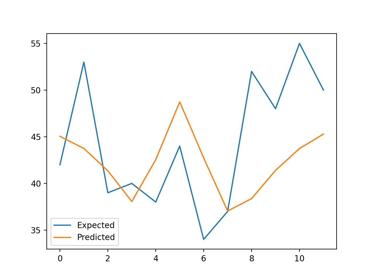
A line plot is created comparing the series of expected values and predicted values for the last 12 months of the dataset.
This gives a geometric interpretation of how well the model performed on the test set.
Line Plot of Expected vs. Births Predicted Using Random Forest
Once a final Random Forest model configuration is chosen, a model can be finalized and used to make a prediction on new data.
This is called an out-of-sample forecast, e.g. predicting beyond the training dataset. This is identical to making a prediction during the evaluation of the model, as we always want to evaluate a model using the same procedure that we expect to use when the model is used to make predictions on new data.
The example below demonstrates fitting a final Random Forest model on all available data and making a one-step prediction beyond the end of the dataset.
1
2
3
4
5
6
7
8
9
10
11
12
13
14
15
16
17
18
19
20
21
22
23
24
25
26
27
28
29
30
31
32
33
34
35
36
37
38
39
40
# finalize model and make a prediction for monthly births with random forest
from numpy import asarray
from pandas import read_csv
from pandas import DataFrame
from pandas import concat
from sklearn.ensemble import RandomForestRegressor
# transform a time series dataset into a supervised learning dataset
Hi Jason…
Thanks a lot for this article.I find most of your articles very useful and informative.
Need your advise-I have a list of products with 3 years historical data as well as other predictor variables.Is there a straightforward way to train all the products in one go and also generate multi-step forecasts to the tune of 18 months.
Did you get a way out for this—How can we do multivariate input (rather than only lags) and have like 4-5 step ahead prediction.Also I have multiple products.How to structure this kind of input for random forest?
Hey, I don’t understand how come testX is like a row of data, and testy is only one value. How come you’re fitting on two such things? I mean normally you would fit on two datasets that are of the same value. I don’t get how testX can be something like: [x, x2, x3, x4, x5, x6] and testy is [y] and you fit them? I mean for each x you should be fitting a y, no? Would appreciate your explanation.
I guess it would just be model.predict(testX) instead of model.predict[testX]), right, so that it predicts for all values of testX instead of just one by one?
Jason, what can i use for random samples in time series data. Which method, which algorithm? I have time series data but samples are so irregular. Thanks for answer and this blog
Thanks, i’m analyzing. Actually, what i mean is, in time series data some observations are trend, seasonal or random sample and i have random one. How can i solve this, any other idea?
Oh man, thanks a lot. So, you say, if my data is really random sample, -i can check this random walk test with your blog- i can’t use any model like AR, ARIMA, random forest, lstm, xgboost, cnn and etc. Probably all of them don’t be useful, right?
And yes, i tried many algorithm which i refer above but none of them didn’t work well
To be honest the post you proposed didn’t help a much.
Do you have more specific advice regarding Covid-19 virus spread prediction?
Any help would be appreciated a lot.
I am doing my undergraduate thesis on predicting time series observations. In my thesis I cover ARIMA, Random Forest, Support Vector Regressor and LSTM models to evaluate the predictive ability.
I used a dataset with measures of RSSI and LQI values (measures for link quality in IEEE 802.15.4 networks) and in my results I obtain in RF, SVR and LSTM a MAPE of >20%, while in ARIMA with Walk Forward Validation I obtain <10%.
However, I tested these same models without any change in time series for the active cases of COVID-19 in Colombia. The results for SVR, RF and LSTM were maintained. I do not know why this happens. Thank you if you can help me.
Hi Jason, Amazing how well this works. I am doing a project using this same boilerplate for predicting water levels. It has multiple variables like temperature, rainfall, hydronomy, volume, and target variable depth to groundwater. Anyways, the model works at using a training set and test set very well, but when I try to fit the model on the entire dataset I get an error about the dimensions
ValueError: Number of features of the model must match the input. Model n_features is 62 and input n_features is 53
There are 9 features in total and the last one is the target, “depth”.
I didnt change anything, used your exact code for training the model on entire dataset to get prediction. Does this particular code not work on multiple variables?
Harvey Benjamin SmithFebruary 14, 2021 at 8:26 am#
I used that way to set up my multivariate data but im still getting the same problem. The number of features going into the model is 79, but the number that its trying to use for the final predition based of the model is only 60. The problem is this line
The training data is all the columns, the t and t-1 for each feature, but according to your code, the final prediction shoud just feed data dimensions from the original dataset, without the lag colunms. I wihs you could show an example for this particular article using a multivariate dataset as well, like you do with all the other time series articles
Hi Jason! First at all thank you so much for share your knowledge, Do you have any example for multi-step forecasting using recursive strategy? For example if I want to predict 12 periods instead?
Thanks for this informative post!
I have a simple doubt but i could not find a clear answer anywhere online. How can i forecast next 1 month(out of sample) using lag variables . e.g. Today i need to make forecast for next 1 month. Since I do not have data available for next 1 month how to approach this problem?
You must define the model and prepare the data based on what you expect to have available at prediction time.
If some data will not be available at prediction time, then do not use it as input when defining your model and preparing your data.
For example, if you want to predict next month but you only have two months ago data, then define your data and model always make prediction based on two months ago data.
Hey, thanks for the tutorial. Since we need to maintain the order of the data for the future prediction, is it correct to assume that when the subset is generated via the sliding window, the bragging (sample with replacement) and the random selection of the subset of features as with the standard RF happens only within that sliding window subset? I guess I am confused that since the order of the data needs to be maintained but then bragging and the random selection of columns for the RF is required, how do those two come into play?
As long as the model is not trained on data in the test set, we’re good. The model itself has no idea of the future/past. Data preparation must handle this correctly.
I would like to ask you, what would I have to do to adapt a Random Forest model for the forecast of a multivariate time series of the type multiple parallel input and multi-step output.
I would like to know, when you refer to start with an appropriate framing of the dataset, if I want to adapt a Random Forest model for the forecast of a multivariate time series of the type multiple parallel input and multi-step output; what would that appropriate framing of the dataset look like?
That is, how should the data be to be able to use the Random Forest for this case, with what type of structure? For example, it would be useful to leave them as in the case of a CNN 1D, of type: X = (# of samples, # of inputs, # of features); y = (# of samples, # of outputs, # of features) ?. Or in what way?
Your blogs are so helpful. I am a novice in ML and need to know from where to start. Would appreciate if you kindly show me a roadmap as to how to navigate through your blogs from the very beginning.
I have been reviewing and I see that the Random Forest models do not normally serve to forecast more than one step into the future, is this correct ?; Or, is it possible to adapt them to make multiple parallel input and multi-step output models?
Thank you for the lesson Dr. Brownlee. I just want to point out in your first definition of walk_forward_regression there is a typo in the return syntax.
it should be return error, test[:, 1-], predictions instead of return error, test[:, 1], predictions. The function in the complete code is correct though.
I really think we would really appreciate a Random Forest example for a multivariate time series even if it was a very simple example, because as you know, there is very little information about multiariant time series. And although, for example, I already organized the data exactly, it is not so intuitive to use this model for a multivariate time series and the execution of the model continues to fail.
Please, if you can give an example like this, it would be of great help.
Thank you for your attention, I am waiting for your answer.
You mentioned that using walk-forward validation is a must, but I am not sure I do understand why.
I understand that in walk-forward validation, the model is first trained using the training data. Then, we evaluate the model on the first step in the test dataset, which is then added to the training data where the model is re-trained on the new training data and so on.
But why is it especially useful for time-series datasets?
You mentioned in another article (linked below for your convenience) that using a normal train-test split or k-cross-validation “would result in optimistically biased results” and the reason was “This is because they assume that there is no relationship between the observations, that each observation is independent.”
But don’t we preserve that when we transform our data and include values at previous timesteps?
For example, if we have our features to be valued at [t-2, t-1] and the label is the value at [t].
So in this case, previous observations are used to estimate the value we are interested in. Therefore I would assume that the relationship between observations is preserved. Is that correct? or what am I missing?
Hi. I would like to ask the n_test = 12 in walk_forward_validation is predicting the final 12 days number of birth right?
mae, y, yhat = walk_forward_validation(data, 12)
The mae for persistence model for predicting the last 12 months stated is 6.7 birth, is this value calculated from predicting the final 12 days to be compared to the model’s mae which is 5.9 births?
With using random trees for forecasting, do you always ever get a prediction that has been inputted into the training set or could you receive a prediction that potentially has never been seen before?
Really enjoying using the resources, they’re helping me dive into ML and undertake some good research for my first Data Science role. I did have a question about data leakage. I understand that the walk forward validation avoids target leakage by not training on future data, but where in the code above would you recommend implementing data scaling so as not to normalise/standardise the entire dataset.
I read your excellent post on data leakage and understood where you’d fit this process into a K-fold cross validation. Just having trouble getting my head around how to adapt this for your custom Walk Forward method.
I’ve been trying to implement that but am going round in circles a bit with adapting your code for the RF model above. Originally I thought I could just fit the scaler to the training data immediately after the train_test_split function in the WF Validation and apply it to both the train/test datasets prior to the loop.
Then I realised that the model refits as a new observation is added to the history doesn’t it? So does the scaler need to be refit within the for loop after this occurs and applied to the test dataset for each iteration? Or is ok to just fit on training once and then apply to test once?
I have two concerns with Random Forest hyperparameters for time series.
1.) If you want to increase the number of decision trees in the n_stimators hyperparameter, in what proportion should this value be increased if you start from 100 and from 1000, from 100 to 100 from 1000 to 1000, or how?
2.) If you have a regression and you want to adjust the number of random characteristics to consider at each division point so that total_input_features / 3 remains, is the hyperparameter max_features the one that must be adjusted? And if this is the case, to adjust it in this way, how should it be configured?
You can do sklearn.ensemble.RandomForestRegressor(max_features=0.33) or sklearn.ensemble.RandomForestRegressor(max_features=int(total_input_features/3.0))
Another question arises, in practice when working with Random Forest to make regression in multivarant and multiparallel time series of several steps, is there a case where I should or is convenient to do some kind of transformation to the data?
Random forest (i.e. decision trees) usually do not need scaling. But if you are considering feature extraction (e.g. PCA), that might be the transform you would do. However, that is dependent on the problem. For example, it is often useful for macroeconomic regression.
Hi Jason, first of all thank you for this blog, I really enjoy it and it is very well explained.
I am trying to use this for a multivariate time series dataset that uses 3 different labels. However, for each subject, the labeling will change from 1 to 3 or to 1 to 2 at some point. I am trying to find which features causes this change in the labeling of my dataset. Is there something like that implemented in the world of machine learning?
Also, this code however, takes the n_test value to determine the test data and it always take the last n_test values of the dataset. Is there anyway to change that and instead, use something in between (when the labeling change occurs) as test? Would that make any sense?
Labelling depends on some random factors. That’s the nature of the label encoder you use. If you don’t like it, you better do it manually: Create a python dict with the label mapping, then use it to replace a column before you feed into the machine learning model.
I was curious if it is possible to compute aggregate statistics of your lag variables? Currently my data is fairly high dimensional and I’d like to limit the number of new features I introduce by incorporating a lag. I’m also attempting to predict rodent behaviors which I feel requires me to have a decently sized window (i.e. 2 seconds) and my data consists of timesteps of 200 ms. My thought was rather than incorporating features for each of those timesteps within that window, I could take some aggregate statistics such as the SD or Mean. Is this common in the world of ML, and how much information do you think I’d lose with this approach?
I am not quite understand what you mean on the aggregate statistics of lag variables. But it makes sense in some model to add new derived features to help the forecast. For example, instead of only the time series, adding the moving average of the time series together to make it a multidimensional is a common trick to help the accuracy.
Thanks for this. Curious, it seems in most non-time series type classification or regression problems, you want to shuffle your data. However, searching through this, I did not see anything about shuffling the data. My thought is that you would never want to shuffle time series data, but I haven’t seen found anything about why you should or shouldn’t shuffle time series data. Just curious your thoughts?
Hi Anthony…you should not shuffle time-series data because deep learning models are learning the correlation and extracting features that are inherent in the data based upon the order of the data. This is why you would not randomly split the data.
Sorry, I probably should have clarified in my previous post, that even after you’ve prepared your data using the “series_to_supervised” function where it creates a sequences of past data and data one step in the future. Would there ever be any good reason to shuffle after this this step and prior to splitting into training and test data?
Hello Jason,
Happy to share that I could run the code for my data.
But I have observed that the MAE in my case remains around 41. I have changed n_estimators from 1000 to 5000. but no change in MAE and remaining around 41. What changes I should do now?
Hi Farjam…The following code definition is set for a stride of 1, however you can alter it to whatever stride you need by changing “n_in” and “n_out” to other values that make sense for your objective.
first of all, thanks for your excelent work and lesson.
I have a question: what if we needed more than one single out-of-sample value, in the end.
I mean, what if we want to predict many days, weeks, years, etc… ahead from our factual historical data last sample?
Should we incorporate our first out-of-sample prediction and restart the whole procsses from the begining or ther’s another better way!
example: Let’s say we have a any sport season that’s is being played. Imagine we have, like, the results of 11 rounds from 50 of that season, and we want to predict the other till the end.
How to tune hyper-parameters for Random Forest in case of walk forward validation? Can we use grid search to optimise hyper-parameters and once best parameters are obained, we again use walk forward validation?
Big time fan of your blogs, and they have been very useful as of late.
I have a similar question to Yogesh. I have read your supplied resource above, and I have a general understanding of how to run a grid search/pipeline with more traditional independent and dependent variables or even with sklearn’s TimeSeriesSplit to create a variety of training and validation sets. I would like to tune my hyper-parameters on the RFR that is looking pretty good with walk forward validation. Is it possible to incorporate walk forward validation into my grid search for tuning the model?
Hi Jason, I find your post and explanation very helpful!
But since I’m new to Python coding and machine learning, how would you write the code to conduct a multi-step forecast, say for 30 steps after the end of the dataset? What would you change in the code?
Hello Jason,
Thank you for all of you hard work. Can you please comment on the following. I noticed in your time series RF examples, the random_forest_forecast method is called once per prediction request (step). But, it also rebuilds the random forest model itself prior to making the prediction. As the prediction window loop gets longer, the model building become more and more based on data it already predicted. Why is it necessary to keep rebuilding the RF model?
For example we have a dataframe with Demand and IsWeekend variables. We use the series_to_supervised function with 10 lags and we would get a dataframe with Demand, IsWeekend and t-n variables (from t-1 to t-10). Do we apply the walkfoward function in the same way? If not, is there any example or reference of this?
so you are regrowing the forest everytime if i am understanding this correctly , so this isn’t true application of the walk forward , or do i got it wrong ?
def random_forest_forecast(train, testX):
# transform list into array
train = asarray(train)
# split into input and output columns
trainX, trainy = train[:, :-1], train[:, -1]
# fit model
model = RandomForestRegressor(n_estimators=1000)
model.fit(trainX, trainy)
# make a one-step prediction
yhat = model.predict([testX])
return yhat[0]
# walk-forward validation for univariate data
def walk_forward_validation(data, n_test):
predictions = list()
# split dataset
train, test = train_test_split(data, n_test)
# seed history with training dataset
history = [x for x in train]
# step over each time-step in the test set
for i in range(len(test)):
# split test row into input and output columns
testX, testy = test[i, :-1], test[i, -1]
# fit model on history and make a prediction
yhat = random_forest_forecast(history, testX)
# store forecast in list of predictions
predictions.append(yhat)
# add actual observation to history for the next loop
history.append(test[i])
# summarize progress
print(‘>expected=%.1f, predicted=%.1f’ % (testy, yhat))
# estimate prediction error
error = mean_absolute_error(test[:, -1], predictions)
return error, test[:, -1], predictions
hi , thanks for taking the time but you didn’t awnser my question wich is a simple one maybe i should reformulate it , in the code above that is yours i belive you are overwriting the old model with a new one each time you expand the data with the test set this isn’t true application of walk forward , my proof is this link from the officiel sklearn site that talks about incremental learning and ràndom forest is not one of them.
hi again now i understand that your code shows the principle of walk forward and not really how you would implement it realistically , part of the confusion came from me not knowing that random forest under sklearn can’t be taught incrementally , i thought you were using the walk forward technique to teach the model incrementally .
Your blog is very informative. I have few queries.
Considering theory developed for random forests for dependent data as per Goehry, 2020; block bootstrap methods are used in place of standard bootstrap methods for i.i.d. data. While implementing randomForest in R or Python for time series data, which bootstrap method is used?
Another query is how does ‘rangerts’ package compare with ‘randomForests’ package?
Hi GT…When implementing random forests in R or Python for time series data, typically a method called “time series cross-validation” is used instead of traditional bootstrapping methods. Time series cross-validation accounts for the temporal dependence in the data by splitting the data into training and testing sets in a sequential manner, ensuring that the model is evaluated on unseen future data.
In R, you can use the caret package for time series cross-validation with the timeslice method. This method splits the data into multiple contiguous training/testing sets.
For Python, libraries like scikit-learn provide functionality for time series cross-validation through the TimeSeriesSplit class.
Regarding your second question, the randomForest package and the ranger package (not rangerts) are both popular implementations of random forests in R. Here’s a comparison:
1. **randomForest package:**
– Developed by Leo Breiman and Adele Cutler, the randomForest package is one of the earliest and most widely-used implementations of random forests in R.
– It provides a simple interface for building random forest models and includes options for tuning parameters such as the number of trees and the number of features considered at each split.
2. **ranger package:**
– The ranger package is a newer implementation of random forests in R.
– It is designed to be faster and more memory-efficient than the randomForest package, particularly for large datasets.
– ranger also includes additional features such as variable importance measures and the ability to handle categorical variables with more than 53 levels.
Overall, both packages are effective for building random forest models in R, but you may prefer ranger for its improved performance and additional features, especially when working with large datasets. However, the choice between the two ultimately depends on your specific requirements and preferences.


Very helpful as always! Thanks for sharing this.
Thanks!
Excellent, thank you
Thanks!
Very informative and excellent article that explains complex concept in simple understandable words. Thank you for sharing this variable knowledge.
You’re welcome.
Excellent, thank you
Thanks.
Thanks for the notebook. How can we do multivariate input (rather than only lags) and have like 4-5 step ahead prediction
I believe the random forest can support multiple output’s directly.
e.g. prepare your data and fit your model.
Hi Jason…
Thanks a lot for this article.I find most of your articles very useful and informative.
Need your advise-I have a list of products with 3 years historical data as well as other predictor variables.Is there a straightforward way to train all the products in one go and also generate multi-step forecasts to the tune of 18 months.
Thanks.
I recommend that you test a suite of different approaches in order to discover what works best for your dataset.
Hi Fawad
Did you get a way out for this—How can we do multivariate input (rather than only lags) and have like 4-5 step ahead prediction.Also I have multiple products.How to structure this kind of input for random forest?
The same function can be used to prepare multivariate data and the same model to model it.
Hi Jason
I’ve been trying to run the program and I get this errors
line 56, in walk_forward_validation
testX, testy = test[i, :-1], test[i, -1]
IndexError: index -1 is out of bounds for axis 1 with size 0
Sorry to hear that, this will help:
https://machinelearningmastery.com/faq/single-faq/why-does-the-code-in-the-tutorial-not-work-for-me
Fantastic, thank you very much. It is understandable, educational and usable even after a rough translation into French 🙂
Thanks!
is there no a simpler function to define walk forward training?
Not that I have found. Most libraries mess it up.
Hey, I don’t understand how come testX is like a row of data, and testy is only one value. How come you’re fitting on two such things? I mean normally you would fit on two datasets that are of the same value. I don’t get how testX can be something like: [x, x2, x3, x4, x5, x6] and testy is [y] and you fit them? I mean for each x you should be fitting a y, no? Would appreciate your explanation.
Thank you.
Good question, I recommend starting here:
https://machinelearningmastery.com/time-series-forecasting-supervised-learning/
How can you do a multi-step prediction with random forest?
Thanks.
I guess it would just be model.predict(testX) instead of model.predict[testX]), right, so that it predicts for all values of testX instead of just one by one?
Random forest supports multiple output regression directly, simply prepare your data and the model will learn it.
Jason, what can i use for random samples in time series data. Which method, which algorithm? I have time series data but samples are so irregular. Thanks for answer and this blog
Not sure I understand sorry, perhaps this will help:
https://machinelearningmastery.com/faq/single-faq/how-do-i-handle-discontiguous-time-series-data
Thanks, i’m analyzing. Actually, what i mean is, in time series data some observations are trend, seasonal or random sample and i have random one. How can i solve this, any other idea?
If it is truely random (e.g. a random walk), then a persistence model may be the best that you can use.
Oh man, thanks a lot. So, you say, if my data is really random sample, -i can check this random walk test with your blog- i can’t use any model like AR, ARIMA, random forest, lstm, xgboost, cnn and etc. Probably all of them don’t be useful, right?
And yes, i tried many algorithm which i refer above but none of them didn’t work well
You’re welcome.
Correct. If the data is random it cannot be predicted. the best you can do is a persistence model (a worst case).
Thanks a so much man, i appreciate
You’re welcome.
Hi Jason,
Thanks for the meaningful post.
I’m working on a project and trying to predict Covid-19 spread in my country next months.
Do you think this method is suitable for time series data like covid – 19 cases?
Thanks,
Agron.
This is a common question that I answer here:
https://machinelearningmastery.com/faq/single-faq/how-can-i-use-machine-learning-to-model-covid-19-data
Hi again Jason,
To be honest the post you proposed didn’t help a much.
Do you have more specific advice regarding Covid-19 virus spread prediction?
Any help would be appreciated a lot.
Thanks in advance,
Agron.
Sorry, i don’t have tutorials on the specific topic.
Hi Jason!
I am doing my undergraduate thesis on predicting time series observations. In my thesis I cover ARIMA, Random Forest, Support Vector Regressor and LSTM models to evaluate the predictive ability.
I used a dataset with measures of RSSI and LQI values (measures for link quality in IEEE 802.15.4 networks) and in my results I obtain in RF, SVR and LSTM a MAPE of >20%, while in ARIMA with Walk Forward Validation I obtain <10%.
However, I tested these same models without any change in time series for the active cases of COVID-19 in Colombia. The results for SVR, RF and LSTM were maintained. I do not know why this happens. Thank you if you can help me.
Sorry, I don’t understand your question, perhaps you can restate it?
Hi Jason,
Thank you very much for this great explanation. Could you please explain how to grid search for a random forest model here
The example here will get you started:
https://machinelearningmastery.com/random-forest-ensemble-in-python/
Hi Jason, Amazing how well this works. I am doing a project using this same boilerplate for predicting water levels. It has multiple variables like temperature, rainfall, hydronomy, volume, and target variable depth to groundwater. Anyways, the model works at using a training set and test set very well, but when I try to fit the model on the entire dataset I get an error about the dimensions
ValueError: Number of features of the model must match the input. Model n_features is 62 and input n_features is 53
There are 9 features in total and the last one is the target, “depth”.
I didnt change anything, used your exact code for training the model on entire dataset to get prediction. Does this particular code not work on multiple variables?
Thanks!
You may need to adapt the code to work with multiple input variables – specifically the preparation of the data.
I believe this will help:
https://machinelearningmastery.com/convert-time-series-supervised-learning-problem-python/
I used that way to set up my multivariate data but im still getting the same problem. The number of features going into the model is 79, but the number that its trying to use for the final predition based of the model is only 60. The problem is this line
row = values[-6:].flatten()
yhat = model.predict(asarray([row]))
The training data is all the columns, the t and t-1 for each feature, but according to your code, the final prediction shoud just feed data dimensions from the original dataset, without the lag colunms. I wihs you could show an example for this particular article using a multivariate dataset as well, like you do with all the other time series articles
I’ll try to provide an additional example in the future.
Did you find a solution to this problem in the end?
Hi Jason! First at all thank you so much for share your knowledge, Do you have any example for multi-step forecasting using recursive strategy? For example if I want to predict 12 periods instead?
Hmmm, I don’t recall sorry. Maybe. I recommend searching the blog (search box at the top of the page).
hello, very good article.
how could I predict the next values that are not in the test dataset? for example, for the next 5 days
Call: model.predict()
Hi Jason,
Thanks for this informative post!
I have a simple doubt but i could not find a clear answer anywhere online. How can i forecast next 1 month(out of sample) using lag variables . e.g. Today i need to make forecast for next 1 month. Since I do not have data available for next 1 month how to approach this problem?
You’re welcome!
You must define the model and prepare the data based on what you expect to have available at prediction time.
If some data will not be available at prediction time, then do not use it as input when defining your model and preparing your data.
For example, if you want to predict next month but you only have two months ago data, then define your data and model always make prediction based on two months ago data.
Hey, thanks for the tutorial. Since we need to maintain the order of the data for the future prediction, is it correct to assume that when the subset is generated via the sliding window, the bragging (sample with replacement) and the random selection of the subset of features as with the standard RF happens only within that sliding window subset? I guess I am confused that since the order of the data needs to be maintained but then bragging and the random selection of columns for the RF is required, how do those two come into play?
As long as the model is not trained on data in the test set, we’re good. The model itself has no idea of the future/past. Data preparation must handle this correctly.
hello Jason, great post!
What’s the difference between using RF and ARIMA to predict time series in this case?
One is an ensemble of decision trees, one is a linear model.
Hi Jason,
Nice article. When I replicate your code then I get an error. Plss lemme know how to fix it.
Code –
# fit model
model = RandomForestRegressor(n_estimators=1000)
model.fit(trainX, trainY)
# construct an input for a new prediction
row = values[-6:].flatten()
# make a one-step prediction
yhat = model.predict(asarray([row]))
print(‘Input: %s, Predicted: %.3f’ % (row, yhat[0]))
Error –
This RandomForestRegressor instance is not fitted yet. Call ‘fit’ with appropriate arguments before using this estimator.
Perhaps these tips will help:
https://machinelearningmastery.com/faq/single-faq/why-does-the-code-in-the-tutorial-not-work-for-me
Hi Jason:
Is it possible that we refer to an example for multivariate time series?
Thanks for your attention.
Sorry, I don’t think I have an example of RF for multivariate time series.
Hi Jason:
I would like to ask you, what would I have to do to adapt a Random Forest model for the forecast of a multivariate time series of the type multiple parallel input and multi-step output.
Thanks for your attention.
Start with an appropriate framing of the dataset, then you should be able to use the model directly.
Perhaps use a little trial and error to learn how to adapt the code for your dataset.
Hi Jason:
I would like to know, when you refer to start with an appropriate framing of the dataset, if I want to adapt a Random Forest model for the forecast of a multivariate time series of the type multiple parallel input and multi-step output; what would that appropriate framing of the dataset look like?
That is, how should the data be to be able to use the Random Forest for this case, with what type of structure? For example, it would be useful to leave them as in the case of a CNN 1D, of type: X = (# of samples, # of inputs, # of features); y = (# of samples, # of outputs, # of features) ?. Or in what way?
Thanks for your attention.
An appropriate framing would have some subset of the data available at prediction time only, e.g. a subset of lag observations.
This can help you prepare the data:
https://machinelearningmastery.com/convert-time-series-supervised-learning-problem-python/
Structure for 1d cnn is identical to the structure for lstms:
https://machinelearningmastery.com/faq/single-faq/what-is-the-difference-between-samples-timesteps-and-features-for-lstm-input
Hi Jason,
Your blogs are so helpful. I am a novice in ML and need to know from where to start. Would appreciate if you kindly show me a roadmap as to how to navigate through your blogs from the very beginning.
Thanks!
Start here:
https://machinelearningmastery.com/start-here/
Hi Jason,
Thank you for your amazing blogs. It really helps to understand the concepts.
I read some posts where it was mentioned that RF models are not good at capturing trends & that seems correct.
Any suggestions to deal with this issue? And don’t we need any preprocessing for time series data like it’s usually done in ML?
You’re welcome.
Try it and see.
Yes, you can difference the data to make it stationary prior to modeling:
https://machinelearningmastery.com/machine-learning-data-transforms-for-time-series-forecasting/
Hi Jason:
I have been reviewing and I see that the Random Forest models do not normally serve to forecast more than one step into the future, is this correct ?; Or, is it possible to adapt them to make multiple parallel input and multi-step output models?
Thanks for your attention.
Try it and see. Yes, you can adapt the example above for anything you like!
Ok, thanks, I´ll try.
Thank you for the lesson Dr. Brownlee. I just want to point out in your first definition of walk_forward_regression there is a typo in the return syntax.
it should be return error, test[:, 1-], predictions instead of return error, test[:, 1], predictions. The function in the complete code is correct though.
Thanks.
Hi, is there a way to make RandomForestRegressor optimize for MASE? I look up the source but the only available criteria are MSE and MAE.
Perhaps you override the class/API with custom code?
Hi Jason,
I really think we would really appreciate a Random Forest example for a multivariate time series even if it was a very simple example, because as you know, there is very little information about multiariant time series. And although, for example, I already organized the data exactly, it is not so intuitive to use this model for a multivariate time series and the execution of the model continues to fail.
Please, if you can give an example like this, it would be of great help.
Thank you for your attention, I am waiting for your answer.
Thanks for the suggestion.
Great tutorial. Why am I getting this error when I try all the codes?
ValueError: could not convert string to float: ‘1959-01-01’
Thanks ahead.
These tips may help:
https://machinelearningmastery.com/faq/single-faq/why-does-the-code-in-the-tutorial-not-work-for-me
Could you say to me how did you solve this problem?
Hi Mojtaba…I am not following your question. Please rephrase so that I may better assist you.
Sorry, my fault. Wrong import config of the csv, sorry! 🙂
No probem!
Hello Jason,
Thanks as always for a great article.
You mentioned that using walk-forward validation is a must, but I am not sure I do understand why.
I understand that in walk-forward validation, the model is first trained using the training data. Then, we evaluate the model on the first step in the test dataset, which is then added to the training data where the model is re-trained on the new training data and so on.
But why is it especially useful for time-series datasets?
You mentioned in another article (linked below for your convenience) that using a normal train-test split or k-cross-validation “would result in optimistically biased results” and the reason was “This is because they assume that there is no relationship between the observations, that each observation is independent.”
But don’t we preserve that when we transform our data and include values at previous timesteps?
For example, if we have our features to be valued at [t-2, t-1] and the label is the value at [t].
So in this case, previous observations are used to estimate the value we are interested in. Therefore I would assume that the relationship between observations is preserved. Is that correct? or what am I missing?
Article: https://machinelearningmastery.com/backtest-machine-learning-models-time-series-forecasting/
It is essential to ensure we don’t train on the future or evaluate on the past, e.g. to offer a fair estimate of model performance on sequenced data.
I understand.
But is sequence still important even after we transform the data to a normal supervised learning problem?
And even when the sequence is important, can we use a simple non-randomized test-split? (e.g. train on first 3 years and test on the fourth year)
Yes.
Yes, this is exactly what walk-forward validation does.
Hi. I would like to ask the n_test = 12 in walk_forward_validation is predicting the final 12 days number of birth right?
mae, y, yhat = walk_forward_validation(data, 12)
The mae for persistence model for predicting the last 12 months stated is 6.7 birth, is this value calculated from predicting the final 12 days to be compared to the model’s mae which is 5.9 births?
Yes.
Hey Jason,
Thank you very much for the nice article!!
While using different data I am encountering this error:
TypeError: float() argument must be a string or a number, not ‘Timestamp’
What can I do?
Thanks!
Looks like you are trying to feed date/times in as data to your model. You cannot.
Hi Jason,
With using random trees for forecasting, do you always ever get a prediction that has been inputted into the training set or could you receive a prediction that potentially has never been seen before?
Thanks,
Bob
I guess it depends on the model and the dataset. It may not matter.
Hi Jason,
Really enjoying using the resources, they’re helping me dive into ML and undertake some good research for my first Data Science role. I did have a question about data leakage. I understand that the walk forward validation avoids target leakage by not training on future data, but where in the code above would you recommend implementing data scaling so as not to normalise/standardise the entire dataset.
I read your excellent post on data leakage and understood where you’d fit this process into a K-fold cross validation. Just having trouble getting my head around how to adapt this for your custom Walk Forward method.
Thank you!
Thanks!
Fit scaler objects on training data and apply to train and test data. You can re-fit scaler objects if/when you refit model objects.
Thanks for getting back to me.
I’ve been trying to implement that but am going round in circles a bit with adapting your code for the RF model above. Originally I thought I could just fit the scaler to the training data immediately after the train_test_split function in the WF Validation and apply it to both the train/test datasets prior to the loop.
Then I realised that the model refits as a new observation is added to the history doesn’t it? So does the scaler need to be refit within the for loop after this occurs and applied to the test dataset for each iteration? Or is ok to just fit on training once and then apply to test once?
Thank you.
You may need to develop a new example for your case.
Hi Jason,
I have two concerns with Random Forest hyperparameters for time series.
1.) If you want to increase the number of decision trees in the n_stimators hyperparameter, in what proportion should this value be increased if you start from 100 and from 1000, from 100 to 100 from 1000 to 1000, or how?
2.) If you have a regression and you want to adjust the number of random characteristics to consider at each division point so that total_input_features / 3 remains, is the hyperparameter max_features the one that must be adjusted? And if this is the case, to adjust it in this way, how should it be configured?
Thanks for your attention.
(1) no rules here, but you need to justify why you do it that way. The best answer is the one that proved by your experiment.
(2) Yes.
But if I want the hyperparameter max_features = total_input_features / 3, how should I configure it ?, like “auto”, “sqrt”, “log2”? …
Are you talking about the parameters to set up the model? I would leave it as default and try it out first.
Yes, I am precisely talking about the parameters to configure the model, if I want max_features = total_input_features / 3, how should I configure it?
Thanks for your attention.
You can do sklearn.ensemble.RandomForestRegressor(max_features=0.33) or sklearn.ensemble.RandomForestRegressor(max_features=int(total_input_features/3.0))
Oh good, I will, but as you say, I will first try the value by default.
Thanks for your help Adrian, it is always very useful for me.
Hi Jason,
Another question arises, in practice when working with Random Forest to make regression in multivarant and multiparallel time series of several steps, is there a case where I should or is convenient to do some kind of transformation to the data?
Thanks for your attention.
Random forest (i.e. decision trees) usually do not need scaling. But if you are considering feature extraction (e.g. PCA), that might be the transform you would do. However, that is dependent on the problem. For example, it is often useful for macroeconomic regression.
Ok thanks for your answer.
Hi Jason, first of all thank you for this blog, I really enjoy it and it is very well explained.
I am trying to use this for a multivariate time series dataset that uses 3 different labels. However, for each subject, the labeling will change from 1 to 3 or to 1 to 2 at some point. I am trying to find which features causes this change in the labeling of my dataset. Is there something like that implemented in the world of machine learning?
Also, this code however, takes the n_test value to determine the test data and it always take the last n_test values of the dataset. Is there anyway to change that and instead, use something in between (when the labeling change occurs) as test? Would that make any sense?
Labelling depends on some random factors. That’s the nature of the label encoder you use. If you don’t like it, you better do it manually: Create a python dict with the label mapping, then use it to replace a column before you feed into the machine learning model.
Hi Jason and Adrian,
I was curious if it is possible to compute aggregate statistics of your lag variables? Currently my data is fairly high dimensional and I’d like to limit the number of new features I introduce by incorporating a lag. I’m also attempting to predict rodent behaviors which I feel requires me to have a decently sized window (i.e. 2 seconds) and my data consists of timesteps of 200 ms. My thought was rather than incorporating features for each of those timesteps within that window, I could take some aggregate statistics such as the SD or Mean. Is this common in the world of ML, and how much information do you think I’d lose with this approach?
Thanks so much for your help!
I am not quite understand what you mean on the aggregate statistics of lag variables. But it makes sense in some model to add new derived features to help the forecast. For example, instead of only the time series, adding the moving average of the time series together to make it a multidimensional is a common trick to help the accuracy.
hi, how the tree split nodes with time series prediction ? we have one feature to work with and predict , in addition to date feature
I don’t think the date is considered in this example.
Thanks for this. Curious, it seems in most non-time series type classification or regression problems, you want to shuffle your data. However, searching through this, I did not see anything about shuffling the data. My thought is that you would never want to shuffle time series data, but I haven’t seen found anything about why you should or shouldn’t shuffle time series data. Just curious your thoughts?
Hi Anthony…you should not shuffle time-series data because deep learning models are learning the correlation and extracting features that are inherent in the data based upon the order of the data. This is why you would not randomly split the data.
Sorry, I probably should have clarified in my previous post, that even after you’ve prepared your data using the “series_to_supervised” function where it creates a sequences of past data and data one step in the future. Would there ever be any good reason to shuffle after this this step and prior to splitting into training and test data?
Hi Anthony…you should not shuffle time series data.
Hej Jason and Adrian
Thank you for the excellent post. Do you have a similar post or study on Multivariate analysis, which includes several factors?
Much appreciate your reply!
Kind regards!
Hi Jing…You may find the following of interest:
https://machinelearningmastery.com/how-to-develop-machine-learning-models-for-multivariate-multi-step-air-pollution-time-series-forecasting/
Hello Jason,
Happy to share that I could run the code for my data.
But I have observed that the MAE in my case remains around 41. I have changed n_estimators from 1000 to 5000. but no change in MAE and remaining around 41. What changes I should do now?
how do I implement def series to supervised with custom stride or step , I want to move more than one step in sliding window .
thx
Hi Farjam…Please see previous reply regarding setting values you need.
Hello Jason
can you help how do I have custom stride I mean to have more than one step to move in def series_to_supervised ?
Hi Farjam…The following code definition is set for a stride of 1, however you can alter it to whatever stride you need by changing “n_in” and “n_out” to other values that make sense for your objective.
def series_to_supervised(data, n_in=1, n_out=1, dropnan=True):
Hi Jason,
first of all, thanks for your excelent work and lesson.
I have a question: what if we needed more than one single out-of-sample value, in the end.
I mean, what if we want to predict many days, weeks, years, etc… ahead from our factual historical data last sample?
Should we incorporate our first out-of-sample prediction and restart the whole procsses from the begining or ther’s another better way!
example: Let’s say we have a any sport season that’s is being played. Imagine we have, like, the results of 11 rounds from 50 of that season, and we want to predict the other till the end.
Hi Enzo…I would recommend first ensuring that the most appropriate method is selected for the given task:
https://machinelearningmastery.com/findings-comparing-classical-and-machine-learning-methods-for-time-series-forecasting/
*[…] data’s last sample
**[…] whole process […] or there’s another better way?
****[…] “any sport’s season” […] others till the end
Hi Enzo…Please clarify your question so that we can better assist you.
Hi Jason!
Thanks for another great lesson!
I have a doubt :
How can I adapt the above code for multi-step forecasts?
How to tune hyper-parameters for Random Forest in case of walk forward validation? Can we use grid search to optimise hyper-parameters and once best parameters are obained, we again use walk forward validation?
Hi Yogesh…the following resource may be of interest:
https://towardsdatascience.com/hyperparameter-tuning-the-random-forest-in-python-using-scikit-learn-28d2aa77dd74
Hello James and Jason,
Big time fan of your blogs, and they have been very useful as of late.
I have a similar question to Yogesh. I have read your supplied resource above, and I have a general understanding of how to run a grid search/pipeline with more traditional independent and dependent variables or even with sklearn’s TimeSeriesSplit to create a variety of training and validation sets. I would like to tune my hyper-parameters on the RFR that is looking pretty good with walk forward validation. Is it possible to incorporate walk forward validation into my grid search for tuning the model?
Thanks. Any help much appreciated.
Hi kmack…Thank you for your feedback and support! You may find the following resources of interest:
https://machinelearningmastery.com/how-to-grid-search-deep-learning-models-for-time-series-forecasting/
https://stats.stackexchange.com/questions/440280/choosing-model-from-walk-forward-cv-for-time-series
Hi Jason, I find your post and explanation very helpful!
But since I’m new to Python coding and machine learning, how would you write the code to conduct a multi-step forecast, say for 30 steps after the end of the dataset? What would you change in the code?
Your reply will be much appreciated!
Hi Bim…You may want to investigate LSTMs for this purpose:
https://machinelearningmastery.com/use-timesteps-lstm-networks-time-series-forecasting/
Hi Jason, I find your post very helpful!
is it right to use random forest or quantile regression random forest for forecasting volatility?
Hi mona…You may find the following resource of interest:
https://www.tandfonline.com/doi/full/10.1080/1331677X.2022.2089192
Hello Jason,
Thank you for all of you hard work. Can you please comment on the following. I noticed in your time series RF examples, the random_forest_forecast method is called once per prediction request (step). But, it also rebuilds the random forest model itself prior to making the prediction. As the prediction window loop gets longer, the model building become more and more based on data it already predicted. Why is it necessary to keep rebuilding the RF model?
Hi Jeff…The model is being updated with new data. So this is actually just an update of the same model.
Hello James,
How we could add an exogenous variable?
For example we have a dataframe with Demand and IsWeekend variables. We use the series_to_supervised function with 10 lags and we would get a dataframe with Demand, IsWeekend and t-n variables (from t-1 to t-10). Do we apply the walkfoward function in the same way? If not, is there any example or reference of this?
Many thanks in advance
Hi dvd…The following resources may be of interest to you:
https://timeseriesreasoning.com/contents/exogenous-and-endogenous-variables/
https://repositorio-aberto.up.pt/bitstream/10216/141197/2/433647.pdf
One query:
Just considering your code:
trainX, trainy = train[:, :-1], train[:, -1]
This doesn’t seem right to me because trainy is contained in trainX
If y = f(X) then shouldn’t y not be included in the trainX set??
Never the less I still get a really good prediction error.
Thank you for your feedback! Best practices for train, test split can be found here:
https://machinelearningmastery.com/training-validation-test-split-and-cross-validation-done-right/
hi , according to this officel link Incremental learning can’t be done to random forrest using scikit-learn:
https://scikit-learn.org/0.15/modules/scaling_strategies.html#incremental-learning
so you are regrowing the forest everytime if i am understanding this correctly , so this isn’t true application of the walk forward , or do i got it wrong ?
def random_forest_forecast(train, testX):
# transform list into array
train = asarray(train)
# split into input and output columns
trainX, trainy = train[:, :-1], train[:, -1]
# fit model
model = RandomForestRegressor(n_estimators=1000)
model.fit(trainX, trainy)
# make a one-step prediction
yhat = model.predict([testX])
return yhat[0]
# walk-forward validation for univariate data
def walk_forward_validation(data, n_test):
predictions = list()
# split dataset
train, test = train_test_split(data, n_test)
# seed history with training dataset
history = [x for x in train]
# step over each time-step in the test set
for i in range(len(test)):
# split test row into input and output columns
testX, testy = test[i, :-1], test[i, -1]
# fit model on history and make a prediction
yhat = random_forest_forecast(history, testX)
# store forecast in list of predictions
predictions.append(yhat)
# add actual observation to history for the next loop
history.append(test[i])
# summarize progress
print(‘>expected=%.1f, predicted=%.1f’ % (testy, yhat))
# estimate prediction error
error = mean_absolute_error(test[:, -1], predictions)
return error, test[:, -1], predictions
Hi Yassine…Have you executed your model? If not, please do and let us know what you find. That will better enable us to guide you on next steps.
hi , thanks for taking the time but you didn’t awnser my question wich is a simple one maybe i should reformulate it , in the code above that is yours i belive you are overwriting the old model with a new one each time you expand the data with the test set this isn’t true application of walk forward , my proof is this link from the officiel sklearn site that talks about incremental learning and ràndom forest is not one of them.
Hi Yassine…Please follow the recommendations as you interpret them from sklearn documentation. Then let us know your findings.
hi again now i understand that your code shows the principle of walk forward and not really how you would implement it realistically , part of the confusion came from me not knowing that random forest under sklearn can’t be taught incrementally , i thought you were using the walk forward technique to teach the model incrementally .
Hi Jason,
Your blog is very informative. I have few queries.
Considering theory developed for random forests for dependent data as per Goehry, 2020; block bootstrap methods are used in place of standard bootstrap methods for i.i.d. data. While implementing randomForest in R or Python for time series data, which bootstrap method is used?
Another query is how does ‘rangerts’ package compare with ‘randomForests’ package?
Thank you in advance.
Hi GT…When implementing random forests in R or Python for time series data, typically a method called “time series cross-validation” is used instead of traditional bootstrapping methods. Time series cross-validation accounts for the temporal dependence in the data by splitting the data into training and testing sets in a sequential manner, ensuring that the model is evaluated on unseen future data.
In R, you can use the
caretpackage for time series cross-validation with thetimeslicemethod. This method splits the data into multiple contiguous training/testing sets.For Python, libraries like
scikit-learnprovide functionality for time series cross-validation through theTimeSeriesSplitclass.Regarding your second question, the
randomForestpackage and therangerpackage (notrangerts) are both popular implementations of random forests in R. Here’s a comparison:1. **randomForest package:**
– Developed by Leo Breiman and Adele Cutler, the
randomForestpackage is one of the earliest and most widely-used implementations of random forests in R.– It provides a simple interface for building random forest models and includes options for tuning parameters such as the number of trees and the number of features considered at each split.
2. **ranger package:**
– The
rangerpackage is a newer implementation of random forests in R.– It is designed to be faster and more memory-efficient than the
randomForestpackage, particularly for large datasets.–
rangeralso includes additional features such as variable importance measures and the ability to handle categorical variables with more than 53 levels.Overall, both packages are effective for building random forest models in R, but you may prefer
rangerfor its improved performance and additional features, especially when working with large datasets. However, the choice between the two ultimately depends on your specific requirements and preferences.Thank you very much for your detailed response. Appreciate it.
can I have a gitlink