One crucial step in machine learning is the choice of model. A suitable model with suitable hyperparameter is the key to a good prediction result. When we are faced with a choice between models, how should the decision be made?
This is why we have cross validation. In scikit-learn, there is a family of functions that help us do this. But quite often, we see cross validation used improperly, or the result of cross validation not being interpreted correctly.
In this tutorial, you will discover the correct procedure to use cross validation and a dataset to select the best models for a project.
After completing this tutorial, you will know:
The significance of training-validation-test split of data and the trade-off in different ratios of the split
The metric to evaluate a model and how to compare models
How to use cross validation to evaluate a model
What should we do if we have a decision based on cross validation
Let’s get started.
Training-validation-test split and cross-validation done right. Photo by Conal Gallagher, some rights reserved.
Tutorial Overview
This tutorial is divided into three parts:
The problem of model selection
Out-of-sample evaluation
Example of the model selection workflow using cross-validation
The problem of model selection
The outcome of machine learning is a model that can do prediction. The most common cases are the classification model and the regression model; the former is to predict the class membership of an input and the latter is to predict the value of a dependent variable based on the input. However, in either case we have a variety of models to choose from. Classification model, for instance, includes decision tree, support vector machine, and neural network, to name a few. Any one of these, depends on some hyperparameters. Therefore, we have to decide on a number of settings before we start training a model.
If we have two candidate models based on our intuition, and we want to pick one to use in our project, how should we pick?
There are some standard metrics we can generally use. In regression problems, we commonly use one of the following:
The metrics page from scikit-learn has a longer, but not exhaustive, list of common evaluations put into different categories. If we have a sample dataset and want to train a model to predict it, we can use one of these metrics to evaluate how efficient the model is.
However, there is a problem; for the sample dataset, we only evaluated the model once. Assuming we correctly separated the dataset into a training set and a test set, and fitted the model with the training set while evaluated with the test set, we obtained only a single sample point of evaluation with one test set. How can we be sure it is an accurate evaluation, rather than a value too low or too high by chance? If we have two models, and found that one model is better than another based on the evaluation, how can we know this is also not by chance?
The reason we are concerned about this, is to avoid surprisingly low accuracy when the model is deployed and used on an entirely new data than the one we obtained, in the future.
Out-of-sample evaluation
The solution to this problem is the training-validation-test split.
The model is initially fit on a training data set, […] Successively, the fitted model is used to predict the responses for the observations in a second data set called the validation data set. […] Finally, the test data set is a data set used to provide an unbiased evaluation of a final model fit on the training data set. If the data in the test data set has never been used in training (for example in cross-validation), the test data set is also called a holdout data set.
— “Training, validation, and test sets”, Wikipedia
The reason for such practice, lies in the concept of preventing data leakage.
“What gets measured gets improved.”, or as Goodhart’s law puts it, “When a measure becomes a target, it ceases to be a good measure.” If we use one set of data to choose a model, the model we chose, with certainty, will do well on the same set of data under the same evaluation metric. However, what we should care about is the evaluation metric on the unseen data instead.
Therefore, we need to keep a slice of data from the entire model selection and training process, and save it for the final evaluation. This slice of data is the “final exam” to our model and the exam questions must not be seen by the model before. Precisely, this is the workflow of how the data is being used:
training dataset is used to train a few candidate models
validation dataset is used to evaluate the candidate models
one of the candidates is chosen
the chosen model is trained with a new training dataset
the trained model is evaluated with the test dataset
In steps 1 and 2, we do not want to evaluate the candidate models once. Instead, we prefer to evaluate each model multiple times with different dataset and take the average score for our decision at step 3. If we have the luxury of vast amounts of data, this could be done easily. Otherwise, we can use the trick of k-fold to resample the same dataset multiple times and pretend they are different. As we are evaluating the model, or hyperparameter, the model has to be trained from scratch, each time, without reusing the training result from previous attempts. We call this process cross validation.
From the result of cross validation, we can conclude whether one model is better than another. Since the cross validation is done on a smaller dataset, we may want to retrain the model again, once we have a decision on the model. The reason is the same as that for why we need to use k-fold in cross-validation; we do not have a lot of data, and the smaller dataset we used previously, had a part of it held out for validation. We believe combining the training and validation dataset can produce a better model. This is what would occur in step 4.
The dataset for evaluation in step 5, and the one we used in cross validation, are different because we do not want data leakage. If they were the same, we would see the same score as we have already seen from the cross validation. Or even worse, the test score was guaranteed to be good because it was part of the data we used to train the chosen model and we have adapted the model for that test dataset.
Once we finished the training, we want to (1) compare this model to our previous evaluation and (2) estimate how it will perform if we deploy it.
We make use of the test dataset that was never used in previous steps to evaluate the performance. Because this is unseen data, it can help us evaluate the generalization, or out-of-sample, error. This should simulate what the model will do when we deploy it. If there is overfitting, we would expect the error to be high at this evaluation.
Similarly, we do not expect this evaluation score to be very different from that we obtained from cross validation in the previous step, if we did the model training correctly. This can serve as a confirmation for our model selection.
Example of the model selection workflow using cross-validation
In the following, we fabricate a regression problem to illustrate how a model selection workflow should be.
First, we use numpy to generate a dataset:
Python
1
2
3
4
5
6
...
# Generate data and plot
N=300
x=np.linspace(0,7*np.pi,N)
smooth=1+0.5*np.sin(x)
y=smooth+0.2*np.random.randn(N)
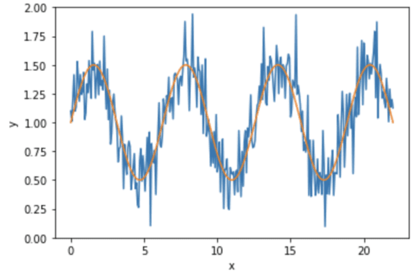
We generate a sine curve and add some noise into it. Essentially, the data is
$$y=1 + 0.5\sin(x) + \epsilon$$
for some small noise signal $\epsilon$. The data looks like the following:
Then we perform a train-test split, and hold out the test set until we finish our final model. Because we are going to use scikit-learn models for regression, and they assumed the input x to be in two-dimensional array, we reshape it here first. Also, to make the effect of model selection more pronounced, we do not shuffle the data in the split. In reality, this is usually not a good idea.
Python
1
2
3
4
...
# Train-test split, intentionally use shuffle=False
In the next step, we create two models for regression. They are namely quadratic:
$$y = c + b\times x + a\times x^2$$
and linear:
$$y = b + a\times x$$
There are no polynomial regression in scikit-learn but we can make use of PolynomialFeatures combined with LinearRegression to achieve that. PolynomialFeatures(2) will convert input $x$ into $1,x,x^2$ and linear regression on these three will find us the coefficients $a,b,c$ in the formula above.
Python
1
2
3
4
...
# Create two models: Quadratic and linear regression
which the key test_score holds the score for each fold. We are using negative root mean square error for the cross validation and the higher the score, the less the error, and hence the better the model.
The above is from the quadratic model. The corresponding test score from the linear model is as follows:
Before we proceed to train our model of choice, we can illustrate what happened. Take the first cross-validation iteration as an example, we can see that the coefficient for quadratic regression is as follows:
Python
1
2
3
4
...
# Let's show the coefficient of the first fitted polynomial regression
# This starts from the constant term and in ascending order of powers
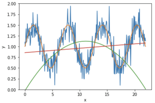
Here we see the red line is the linear regression while the green line is from quadratic regression. We can see the quadratic curve is immensely off from the input data (blue curve) at two ends.
Since we decided to use linear model for regression, we need to re-train the model and test it using our held out test data.
Python
1
2
3
4
5
...
# Retrain the model and evaluate
linreg.fit(X_train,y_train)
print("Test set RMSE:",mean_squared_error(y_test,linreg.predict(X_test),squared=False))
Here, since scikit-learn will clone a new model on every iteration of cross validation, the model we created remain untrained after cross validation. Otherwise, we should reset the model by cloning a new one using linreg = sklearn.base.clone(linreg). But from above, we see that we obtained the root mean squared error of 0.440 from our test set while the score we obtained from cross validation is 0.446. This is not too much of a difference, and hence, we concluded that this model should see an error of similar magnitude for new data.
Tying all these together, the complete example is listed below.
In this tutorial, you discovered how to do training-validation-test split of dataset and perform k-fold cross validation to select a model correctly and how to retrain the model after the selection.
Specifically, you learned:
The significance of training-validation-test split to help model selection
How to evaluate and compare machine learning models using k-fold cross-validation on a training set.
How to retrain a model after we select from the candidates based on the advice from cross-validation
How to use test set to confirm our model selection
This is another fantastic article! If I may, I have a couple of questions based on what you have here:
1) What situations, if any, is it beneficial to set Shuffle=False?
2) In your experience, what do you consider a dataset of sufficient enough size to warrant holdout exclusively instead of cross-validation?
This is most definitely an aspect of machine learning I want to master because I’ve only been doing this sort of work for about a year. Thank you very much for your time!
(1) You should almost always shuffle. Except for time series, because you will distort the time axis
(2) Depends on your model complexity. For some mysterious reason, there is a magic number 30 in statistics. So my ballpark estimation would be 30x the number of parameters in the model to be good enough for one holdout.
in summary:
1. CV on the whole dataset with multiple models
2. choose best model from step 1
3. fit & predict using data from train test split with model from step 2
is that correct? if so, sometime i see an example where CV is done in training data then the best model is used to predict in testing data. is that also correcct?
Either way is fine in my opinion. But using only training data for CV is preferred and more practical. Think that test data is something I will get tomorrow. So I will use CV using today’s data and find the best model. Then build it. Then test it tomorrow and convince people it is good (because I didn’t know the test data when I build it and it can predict well). Then I can put the trained model into production use next week.
Hi Adrian, good article! It might be worth mentioning that one should never do oversampling (including SMOTE, etc.) *before* doing a train-test-validation split or before doing cross-validation on the oversampled data. The correct way to do oversampling with cross-validation is to do the oversampling *inside* the cross-validation loop, oversampling *only* the training folds being used in that particular iteration of cross-validation. Otherwise you end up with some of the duplicate or dependent oversampled instances appearing in both the train folds and the validation fold, which makes them not independent and partially invalidates and biases the cross-validation. One way to do it correctly is to build a pipeline with the oversampling built into it using create_pipeline_imb() from the imbalanced-learn package and then perform cross validation (e.g. GridSearchCV) on that pipeline as your model, although I haven’t tried this particular method.
Thanks for your suggestion. That’s correct. In fact, what you described is called data leakage and it is something we should avoid in validation (otherwise your validation score is not accurate).
After step 3 (“one of the candidates is chosen”) you wrote:
4. the chosen model is trained with a new training dataset
5. the trained model is evaluated with the test dataset
Question: Should there be a step between 4) and 5) where you perform cross-validation and hyperparameter tuning again on the selected model? (Since you’re working with a different training set then.)
Hello Sir. What is the relation between the “cross_validate” of Sklearn and “Kfold” of sklearn? Are they both similar functions used to perform the same kind of KFold cross validation, or is there a difference between the two functions? I am asking this because of your other tutorial which mentions configuring Kfold cross-validation explicitly.


")

Adrian,
This is another fantastic article! If I may, I have a couple of questions based on what you have here:
1) What situations, if any, is it beneficial to set Shuffle=False?
2) In your experience, what do you consider a dataset of sufficient enough size to warrant holdout exclusively instead of cross-validation?
This is most definitely an aspect of machine learning I want to master because I’ve only been doing this sort of work for about a year. Thank you very much for your time!
(1) You should almost always shuffle. Except for time series, because you will distort the time axis
(2) Depends on your model complexity. For some mysterious reason, there is a magic number 30 in statistics. So my ballpark estimation would be 30x the number of parameters in the model to be good enough for one holdout.
hi!
in summary:
1. CV on the whole dataset with multiple models
2. choose best model from step 1
3. fit & predict using data from train test split with model from step 2
is that correct? if so, sometime i see an example where CV is done in training data then the best model is used to predict in testing data. is that also correcct?
thank you as always, mr adrian tam!
Either way is fine in my opinion. But using only training data for CV is preferred and more practical. Think that test data is something I will get tomorrow. So I will use CV using today’s data and find the best model. Then build it. Then test it tomorrow and convince people it is good (because I didn’t know the test data when I build it and it can predict well). Then I can put the trained model into production use next week.
i see then. thank you so much sir!
Hi ,
when do you say training data you mean the X (independent variable) is fed into cross-val?
Or you use the train test split and you feed into cross-val the x_train, y_train?
Thanks
Hi Adrian, good article! It might be worth mentioning that one should never do oversampling (including SMOTE, etc.) *before* doing a train-test-validation split or before doing cross-validation on the oversampled data. The correct way to do oversampling with cross-validation is to do the oversampling *inside* the cross-validation loop, oversampling *only* the training folds being used in that particular iteration of cross-validation. Otherwise you end up with some of the duplicate or dependent oversampled instances appearing in both the train folds and the validation fold, which makes them not independent and partially invalidates and biases the cross-validation. One way to do it correctly is to build a pipeline with the oversampling built into it using create_pipeline_imb() from the imbalanced-learn package and then perform cross validation (e.g. GridSearchCV) on that pipeline as your model, although I haven’t tried this particular method.
Correction, that should be make_pipeline_imb(), not create_pipeline_imb().
Thanks for your suggestion. That’s correct. In fact, what you described is called data leakage and it is something we should avoid in validation (otherwise your validation score is not accurate).
How can I explain the fact that test accuracy is much higher than train accuracy?
Most likely by chance.
Hi, thanks for the tutorial!
After step 3 (“one of the candidates is chosen”) you wrote:
4. the chosen model is trained with a new training dataset
5. the trained model is evaluated with the test dataset
Question: Should there be a step between 4) and 5) where you perform cross-validation and hyperparameter tuning again on the selected model? (Since you’re working with a different training set then.)
Hi S…that may in fact increase training performance and accuracy.
Hello Sir. What is the relation between the “cross_validate” of Sklearn and “Kfold” of sklearn? Are they both similar functions used to perform the same kind of KFold cross validation, or is there a difference between the two functions? I am asking this because of your other tutorial which mentions configuring Kfold cross-validation explicitly.
Thanks in advance for the clarification.
Hi Priya…the following resource may help add clarity:
https://medium.com/gustavorsantos/how-to-do-cross-validation-kfold-and-grid-search-in-python-e570cdb20a28
Thank you very much for the reference article!
Thank you very much for the reference article.
Dear Jason,
Just to be clear
Step 2 validation dataset is used to evaluate the candidate models. Here, validation dataset = y_train
Step 4 the chosen model is trained with a new training dataset. Here, a new training dataset = X_train + y_train
Are they correct?
Hi Yunhao…Thank you for your feedback! Your understanding is correct.
Hello,
Thanks for the tutorial.
I have 2 questions, please.
Q1: We cloned the linreg model in line 61. Why?
Q2: Why we didn’t simply write in line 61
linreg = LinearRegression()
like we previously did in line 30?
Thanks