How do you know if your time series problem is predictable?
This is a difficult question with time series forecasting. There is a tool called a random walk that can help you understand the predictability of your time series forecast problem.
In this tutorial, you will discover the random walk and its properties in Python.
After completing this tutorial, you will know:
- What the random walk is and how to create one from scratch in Python.
- How to analyze the properties of a random walk and recognize when a time series is and is not a random walk.
- How to make predictions for a random walk.
Kick-start your project with my new book Time Series Forecasting With Python, including step-by-step tutorials and the Python source code files for all examples.
Let’s get started.
- Updated Sept/2019: Updated examples to use latest API.

A Gentle Introduction to the Random Walk for Times Series Forecasting with Python
Photo by Sam valadi, some rights reserved.
Random Series
The Python standard library contains the random module that provides access to a suite of functions for generating random numbers.
The randrange() function can be used to generate a random integer between 0 and an upper limit.
We can use the randrange() function to generate a list of 1,000 random integers between 0 and 10. The example is listed below.
|
1 2 3 4 5 6 7 |
from random import seed from random import randrange from matplotlib import pyplot seed(1) series = [randrange(10) for i in range(1000)] pyplot.plot(series) pyplot.show() |
Running the example plots the sequence of random numbers.
It’s a real mess. It looks nothing like a time series.
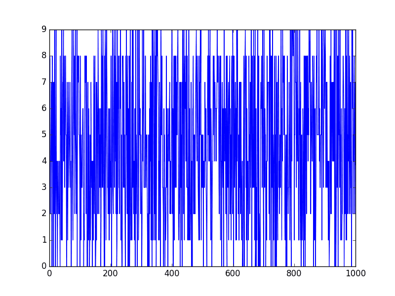
Random Series
This is not a random walk. It is just a sequence of random numbers.
A common mistake that beginners make is to think that a random walk is a list of random numbers, and this is not the case at all.
Stop learning Time Series Forecasting the slow way!
Take my free 7-day email course and discover how to get started (with sample code).
Click to sign-up and also get a free PDF Ebook version of the course.
Random Walk
A random walk is different from a list of random numbers because the next value in the sequence is a modification of the previous value in the sequence.
The process used to generate the series forces dependence from one-time step to the next. This dependence provides some consistency from step-to-step rather than the large jumps that a series of independent, random numbers provides.
It is this dependency that gives the process its name as a “random walk” or a “drunkard’s walk”.
A simple model of a random walk is as follows:
- Start with a random number of either -1 or 1.
- Randomly select a -1 or 1 and add it to the observation from the previous time step.
- Repeat step 2 for as long as you like.
More succinctly, we can describe this process as:
|
1 |
y(t) = B0 + B1*X(t-1) + e(t) |
Where y(t) is the next value in the series. B0 is a coefficient that if set to a value other than zero adds a constant drift to the random walk. B1 is a coefficient to weight the previous time step and is set to 1.0. X(t-1) is the observation at the previous time step. e(t) is the white noise or random fluctuation at that time.
We can implement this in Python by looping over this process and building up a list of 1,000 time steps for the random walk. The complete example is listed below.
|
1 2 3 4 5 6 7 8 9 10 11 12 |
from random import seed from random import random from matplotlib import pyplot seed(1) random_walk = list() random_walk.append(-1 if random() < 0.5 else 1) for i in range(1, 1000): movement = -1 if random() < 0.5 else 1 value = random_walk[i-1] + movement random_walk.append(value) pyplot.plot(random_walk) pyplot.show() |
Running the example creates a line plot of the random walk.
We can see that it looks very different from our above sequence of random numbers. In fact, the shape and movement looks like a realistic time series for the price of a security on the stock market.
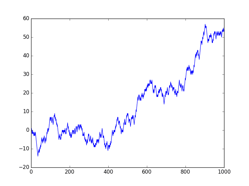
Random Walk Line Plot
In the next sections, we will take a closer look at the properties of a random walk. This is helpful because it will give you context to help identify whether a time series you are analyzing in the future might be a random walk.
Let’s start by looking at the autocorrelation structure.
Random Walk and Autocorrelation
We can calculate the correlation between each observation and the observations at previous time steps. A plot of these correlations is called an autocorrelation plot or a correlogram.
Given the way that the random walk is constructed, we would expect a strong autocorrelation with the previous observation and a linear fall off from there with previous lag values.
We can use the autocorrelation_plot() function in Pandas to plot the correlogram for the random walk.
The complete example is listed below.
Note that in each example where we generate the random walk we use the same seed for the random number generator to ensure that we get the same sequence of random numbers, and in turn the same random walk.
|
1 2 3 4 5 6 7 8 9 10 11 12 13 |
from random import seed from random import random from matplotlib import pyplot from pandas.plotting import autocorrelation_plot seed(1) random_walk = list() random_walk.append(-1 if random() < 0.5 else 1) for i in range(1, 1000): movement = -1 if random() < 0.5 else 1 value = random_walk[i-1] + movement random_walk.append(value) autocorrelation_plot(random_walk) pyplot.show() |
Running the example, we generally see the expected trend, in this case across the first few hundred lag observations.
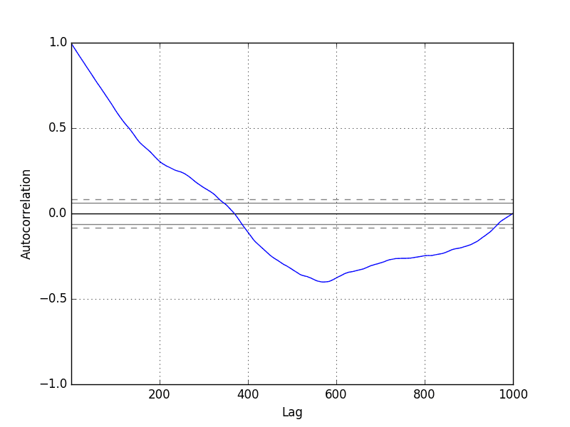
Random Walk Correlogram Plot
Random Walk and Stationarity
A stationary time series is one where the values are not a function of time.
Given the way that the random walk is constructed and the results of reviewing the autocorrelation, we know that the observations in a random walk are dependent on time.
The current observation is a random step from the previous observation.
Therefore we can expect a random walk to be non-stationary. In fact, all random walk processes are non-stationary. Note that not all non-stationary time series are random walks.
Additionally, a non-stationary time series does not have a consistent mean and/or variance over time. A review of the random walk line plot might suggest this to be the case.
We can confirm this using a statistical significance test, specifically the Augmented Dickey-Fuller test.
We can perform this test using the adfuller() function in the statsmodels library. The complete example is listed below.
|
1 2 3 4 5 6 7 8 9 10 11 12 13 14 15 16 17 18 |
from random import seed from random import random from statsmodels.tsa.stattools import adfuller # generate random walk seed(1) random_walk = list() random_walk.append(-1 if random() < 0.5 else 1) for i in range(1, 1000): movement = -1 if random() < 0.5 else 1 value = random_walk[i-1] + movement random_walk.append(value) # statistical test result = adfuller(random_walk) print('ADF Statistic: %f' % result[0]) print('p-value: %f' % result[1]) print('Critical Values:') for key, value in result[4].items(): print('\t%s: %.3f' % (key, value)) |
The null hypothesis of the test is that the time series is non-stationary.
Running the example, we can see that the test statistic value was 0.341605. This is larger than all of the critical values at the 1%, 5%, and 10% confidence levels. Therefore, we can say that the time series does appear to be non-stationary with a low likelihood of the result being a statistical fluke.
|
1 2 3 4 5 6 |
ADF Statistic: 0.341605 p-value: 0.979175 Critical Values: 5%: -2.864 1%: -3.437 10%: -2.568 |
We can make the random walk stationary by taking the first difference.
That is replacing each observation as the difference between it and the previous value.
Given the way that this random walk was constructed, we would expect this to result in a time series of -1 and 1 values. This is exactly what we see.
The complete example is listed below.
|
1 2 3 4 5 6 7 8 9 10 11 12 13 14 15 16 17 18 19 |
from random import seed from random import random from matplotlib import pyplot # create random walk seed(1) random_walk = list() random_walk.append(-1 if random() < 0.5 else 1) for i in range(1, 1000): movement = -1 if random() < 0.5 else 1 value = random_walk[i-1] + movement random_walk.append(value) # take difference diff = list() for i in range(1, len(random_walk)): value = random_walk[i] - random_walk[i - 1] diff.append(value) # line plot pyplot.plot(diff) pyplot.show() |
Running the example produces a line plot showing 1,000 movements of -1 and 1, a real mess.
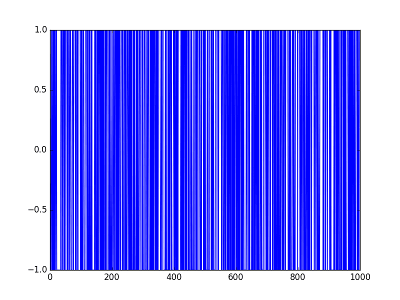
Random Walk Difference Line Plot
This difference graph also makes it clear that really we have no information to work with here other than a series of random moves.
There is no structure to learn.
Now that the time series is stationary, we can recalculate the correlogram of the differenced series. The complete example is listed below.
|
1 2 3 4 5 6 7 8 9 10 11 12 13 14 15 16 17 18 19 20 |
from random import seed from random import random from matplotlib import pyplot from pandas.plotting import autocorrelation_plot # create random walk seed(1) random_walk = list() random_walk.append(-1 if random() < 0.5 else 1) for i in range(1, 1000): movement = -1 if random() < 0.5 else 1 value = random_walk[i-1] + movement random_walk.append(value) # take difference diff = list() for i in range(1, len(random_walk)): value = random_walk[i] - random_walk[i - 1] diff.append(value) # line plot autocorrelation_plot(diff) pyplot.show() |
Running the example, we can see no significant relationship between the lagged observations, as we would expect from the way the random walk was generated.
All correlations are small, close to zero and below the 95% and 99% confidence levels (beyond a few statistical flukes).
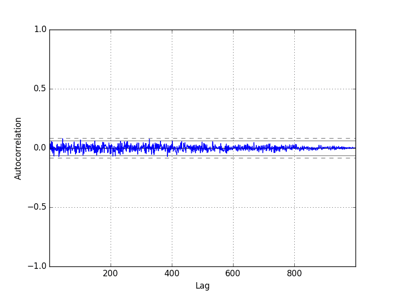
Random Walk Differenced Correlogram Plot
Predicting a Random Walk
A random walk is unpredictable; it cannot reasonably be predicted.
Given the way that the random walk is constructed, we can expect that the best prediction we could make would be to use the observation at the previous time step as what will happen in the next time step.
Simply because we know that the next time step will be a function of the prior time step.
This is often called the naive forecast, or a persistence model.
We can implement this in Python by first splitting the dataset into train and test sets, then using the persistence model to predict the outcome using a rolling forecast method. Once all predictions are collected for the test set, the mean squared error is calculated.
|
1 2 3 4 5 6 7 8 9 10 11 12 13 14 15 16 17 18 19 20 21 22 23 |
from random import seed from random import random from sklearn.metrics import mean_squared_error # generate the random walk seed(1) random_walk = list() random_walk.append(-1 if random() < 0.5 else 1) for i in range(1, 1000): movement = -1 if random() < 0.5 else 1 value = random_walk[i-1] + movement random_walk.append(value) # prepare dataset train_size = int(len(random_walk) * 0.66) train, test = random_walk[0:train_size], random_walk[train_size:] # persistence predictions = list() history = train[-1] for i in range(len(test)): yhat = history predictions.append(yhat) history = test[i] error = mean_squared_error(test, predictions) print('Persistence MSE: %.3f' % error) |
Running the example estimates the mean squared error of the model as 1.
This too is expected, given that we know that the variation from one time step to the next is always going to be 1, either in the positive or negative direction, and the square of this expected error is 1 (1^2 = 1).
|
1 |
Persistence MSE: 1.000 |
Another error that beginners to the random walk make is to assume that if the range of error (variance) is known, then we can make predictions using a random walk generation type process.
That is, if we know the error is either -1 or 1, then why not make predictions by adding a randomly selected -1 or 1 to the previous value.
We can demonstrate this random prediction method in Python below.
|
1 2 3 4 5 6 7 8 9 10 11 12 13 14 15 16 17 18 19 20 21 22 23 |
from random import seed from random import random from sklearn.metrics import mean_squared_error # generate the random walk seed(1) random_walk = list() random_walk.append(-1 if random() < 0.5 else 1) for i in range(1, 1000): movement = -1 if random() < 0.5 else 1 value = random_walk[i-1] + movement random_walk.append(value) # prepare dataset train_size = int(len(random_walk) * 0.66) train, test = random_walk[0:train_size], random_walk[train_size:] # random prediction predictions = list() history = train[-1] for i in range(len(test)): yhat = history + (-1 if random() < 0.5 else 1) predictions.append(yhat) history = test[i] error = mean_squared_error(test, predictions) print('Random MSE: %.3f' % error) |
Running the example, we can see that indeed the algorithm results in a worse performance than the persistence method, with a mean squared error of 1.765.
|
1 |
Random MSE: 1.765 |
Persistence, or the naive forecast, is the best prediction we can make for a random walk time series.
Is Your Time Series a Random Walk?
Your time series may be a random walk.
Some ways to check if your time series is a random walk are as follows:
- The time series shows a strong temporal dependence that decays linearly or in a similar pattern.
- The time series is non-stationary and making it stationary shows no obviously learnable structure in the data.
- The persistence model provides the best source of reliable predictions.
This last point is key for time series forecasting. Baseline forecasts with the persistence model quickly flesh out whether you can do significantly better. If you can’t, you’re probably working with a random walk.
Many time series are random walks, particularly those of security prices over time.
The random walk hypothesis is a theory that stock market prices are a random walk and cannot be predicted.
A random walk is one in which future steps or directions cannot be predicted on the basis of past history. When the term is applied to the stock market, it means that short-run changes in stock prices are unpredictable.
— Page 26, A Random Walk down Wall Street: The Time-tested Strategy for Successful Investing
The human mind sees patterns everywhere and we must be vigilant that we are not fooling ourselves and wasting time by developing elaborate models for random walk processes.
Further Reading
Below are some further resources if you would like to go deeper on Random Walks.
- A Random Walk down Wall Street: The Time-tested Strategy for Successful Investing
- The Drunkard’s Walk: How Randomness Rules Our Lives
- Section 7.3 Evaluating Predictability, Practical Time Series Forecasting with R: A Hands-On Guide
- Section 4.3 Random Walks, Introductory Time Series with R.
- Random Walk on Wikipedia
- Random walk model by Robert F. Nau
Summary
In this tutorial, you discovered how to explore the random walk with Python.
Specifically, you learned:
- How to create a random walk process in Python.
- How to explore the autocorrelation and non-stationary structure of a random walk.
- How to make predictions for a random walk time series.
Do you have any questions about random walks, or about this tutorial?
Ask your questions in the comments below.
Want to Develop Time Series Forecasts with Python?

Develop Your Own Forecasts in Minutes
...with just a few lines of python codeDiscover how in my new Ebook:
Introduction to Time Series Forecasting With Python
It covers self-study tutorials and end-to-end projects on topics like: Loading data, visualization, modeling, algorithm tuning, and much more...
Finally Bring Time Series Forecasting to
Your Own Projects
Skip the Academics. Just Results.


Looking forward to the book. 🙂
Thanks Nader.
Very interesting, thank you ! Could we find the same in sas or R code ?
Thanks in advance !
I’m glad you found it interesting Doumbia.
Sorry, I don’t have examples of a random walk in R or SAS.
That was a very amazing post! Congratulations & Thanks!
Thanks daniel.
Fantastic! Much appreciated.
Thanks Eddmond.
y(t) = B0 + B1*X(t-1) + e(t)
A bit confused with this. Shouldn’t it be
y(t) = B0 + B1*y(t-1) + e(t)
Yes, one and the same. I am used to the supervised learning framing of the problem, sorry.
Informative post!
Thanks
Thanks Samih.
Really interesting. Well done!
Thanks Fabio.
Yes, like Nader I am looking forward to the book. Thanks for the insight
Thanks K. W. Famolu.
Amazing post. In fact it will help many people like me (no hardcore statistical/mathematical background) who are trying to learn time series analysis and prediction.
Thank you Jason. Very much appreciated.
You’re welcome Aninda, glad to hear it!
Just some comments as I hear that stock data is a random walk always. It looks pretty much a random walk and a simple next day prediction might be so if not enough features involved.
If anyone has looked a stock data long enough, knows that those breakpoints, short squeezes, stop loss and so on are causing typical patterns, which can be kept random walk but definitely are not. And at least even some “next” day values can be taught for neural network quite nice, example of one LSTM model although that can be more or less learned internal memory of every value. Nice train set fit anyway:
http://pvoodoo.blogspot.com/2017/01/expected-aimlnn-results.html
Thanks for the note Marko.
interesting issue.
But if seed is same for both train and test, I think that it is not enough good about random walk issue.
I am looking forward to other reports about it.
Thank you
Hi Jason, very informative and interesting article. I agree that some time-series is random-walk especially financial instrument prices, I am actually trying to build a model just to play around, looking at one of your articles on keras predicting time-series, my only premise for trying is that, ‘random is nothing but complex computation of variables that cannot be computed with current technology or techniques and hence,unpredictable’. So far, I can get a convergence of upto one standard deviation, out-of-sample prediction is way too deviated and not useful. Thanks
Best of luck with your project!
Sir, thanks for your tutorial. Would you like to make tutorial on cell sperm detection through Deep Neural Network Model and training this on any own data. If you have on this so please share the link. Thanks
ADF Statistic: 0.341605
p-value: 0.979175
Critical Values:
5%: -2.864
1%: -3.437
10%: -2.568
The p-value and the test statistic here suggest that we reject H0 (Unit-room, non-stationary) and accept the alternative (Stationary). I am a bit confused as you have stated the opposite.
Are you sure?
I say that the series is not stationary (e.g. reject H0):
Hi jason , this is the output of analyzing my time-series using your approach ,
ADF Statistic: -21.866782
p-value: 0.000000
Critical Values:
1%: -3.430
5%: -2.862
10%: -2.567
Is my time series a random walk ?
The test only comments on whether your data is stationary.
Your data does look stationary from that result.
Can I conclude that my time series is not a random walk?
If you can do better than persistence with a predictive model.
Hello Jason,
Thank you for your awesome tutorials, they really help a lot.
I wanted to ask you whether there’s a way to remove random walks from our data (I know that data is either a random walk or not, but maybe make it less random etc.) or any likely sort of thing?
Thanks in advance.
Not as far as I know.
Hi Jason. Thanks for the useful post.
Now I know how to produce a Random Walk series but I’d like to know if I have a time series which follows random walk model, how to forecast its future amounts.
Thanks in advance.
Perhaps check the ACF/PACF plots and confirm that there are is no correlation.
Also try modeling and confirm no model can out-perform persistence.
Hi Jason,
How many data points are good enough for random walk and do statistical test on them. For example if I work on some time series involving patients where each patient has around 8 timesteps then do I need to see random walk for each patient or how can I combine them as each may have different trend.
Good question, not sure. More than 8, maybe 30+
When we are looking at different patients is it same like forecasting for multiple sites. In a link
https://machinelearningmastery.com/faq/single-faq/how-to-develop-forecast-models-for-multiple-sites/
you’ve some suggestions there.
Do you have any posts or example explaining for this prediction for multiple sites e.g. how to make group or hybrid approach etc.
No sorry, it would be specific to your dataset, I would expect.
The random walk data goes negative. How would you suggest this be managed? Not many stock prices actually go negative. Many other data won’t go negative.
It is not a model of stock prices specifically, it is a simulated example of a random walk.
The short term movement in stock prices is a different example of a random walk.
Hi Jason,
I have over 100+ features and 1 output variable (classification) problem that I am trying to address using LSTM. Even though my features are time series the classification decision is done using a different set of parameters.
Do we need to validate random walk when we have multiple input features and 3 possible output classes? If yes, do you have a tutorial for the same as this one deals with regression
Thanks in advance for your help
I forgot to mention it’s a time series classification problem
If you have output classes, it sounds like a time series classification problem.
Perhaps start here instead:
https://machinelearningmastery.com/start-here/#deep_learning_time_series
#Random Walk
Hi Jason, I am going through your book but I am having trouble replacing your TimeSeries sample data with mine in your code. How can replace your sample code without breaking it. Suppose my TimeSeries data source is called ‘series.
Thanks
-Gonzalo
What problem are you having exactly?
Hi Jason,
excellent post !
How is the situation with some time dependent drift component (ala B0(t) != const, ie. piecewise constant), how would you analyse these kind of process ?
Are such questions covered in your book ?
Healthy greetings from Vienna
Bernd
Good question. No, sorry, I don’t have more on analyzing random walks. This tutorial is just designed to introduce the concept.
To dive deeper, I recommend the references listed in the “further reading” section.
Hi Jason,
Really nice post! What about outliers? For example, in sales volume forecasting, a single customer can purchase a large volume and suddenly increase the volume from one week to another. Such outliers potentially determine if a signal can be forecasted and finally beats the naive forecast.
How would you deal with outliers in time-series data? Would clipping the extreme values be a good method?
Best Regards,
Rudiger
Good question.
Yes, you can try deleting, ignoring, clipping, etc, outliers and see which approach works best for your chosen model and dataset.
history = train[-1]
for i in range(len(test)):
yhat = history
predictions.append(yhat)
history = test[i]
you practically add the test data to the prediction but one lag shift as you start the prediction with the last train value.
how is it a prediction when you use the same test data but shifted?
Thanks,
peter
Yes, this is called walk-forward validation and is a standard approach for evaluating time series forecasting models, you can get started with these ideas here:
https://machinelearningmastery.com/backtest-machine-learning-models-time-series-forecasting/
thanks for a nice clear explanation. But shouldn’t the figure Random Walk Differenced Correlogram Plot show a value of 1.0 at zero lag? That said, I am not experienced with python programming, so I don’t know whether what you are showing is the same as the autocorrelation function for the first-differenced random walk series.
Yes, the correlation for t-1 in a random walk is 1.0.
I follow all your posts. You make the difference. Thanks for sharing this amazing guide.
Thanks.
Once in your tutorials, you used the time series of daily-total-femal-births in California. I’m working on that series and I want to know if this is a random walk series or not
I don’t think it is as we can make good predictions on that dataset.
Thank you for the valuable tutorial. I have used the methods in this tutorial to find out is my time series data random walk or not. It turns out that my time series is a random walk. As we know that when a time series is a random walk you cannot use deep learning for time series forecasting. In such scenarios what alternatives do we have to deep learning based forecasting?
If your data is a random walk, you cannot predict. The best you can do is a persistence model.
Hi Jason,
I have a series where the p-value of AD Fuller test is 1. I took the 1st difference of the series, the p value for this is series is 0.7,which still indicates non stationary. Does this mean that the series I am working is not random walk? If so, how to detect what it is.
Thank you and regards,
Sanjeet
Hi Sanjeet…The following resource may help add clarity:
https://www.machinelearningplus.com/time-series/augmented-dickey-fuller-test/
Hi Jason,
I am a little bit confused about the prediction section where you assume that the latest forecast can be used for the next step prediction. This prediction is just to predict one step ahead but what if we would like to predict for one year? I think the latest observation will be used as a constant prediction for that.
Hi Habib…You are correct, and this distinction is important to clarify.
The **random walk model** is a simple statistical method that assumes the best prediction for the next time step is the latest observed value. This approach can be extended to longer forecasting horizons, but it inherently operates on the assumption that the most recent observation is a sufficient representation of the future trend.
### One-Step vs. Multi-Step Forecasting:
1. **One-Step Forecasting:**
– For one-step-ahead predictions, the random walk uses the latest observed value \( y_t \) as the prediction for the next time step \( y_{t+1} \).
2. **Multi-Step Forecasting (e.g., one year):**
– If we want to predict multiple steps ahead (e.g., a year, assuming monthly data, this would be 12 steps), the random walk model assumes that the last observed value is used as the prediction for all future steps:
\[
\hat{y}_{t+h} = y_t, \, \forall h \geq 1
\]
– Here, \( \hat{y}_{t+h} \) is the predicted value at step \( t+h \), and \( y_t \) is the last observation.
This is why in random walk forecasting:
– The prediction for one-step ahead is \( y_{t+1} = y_t \).
– The prediction for two-steps ahead is \( y_{t+2} = y_t \), and so on.
In essence, the random walk assumes no trend, seasonality, or additional information in the data, treating the latest value as the most reliable guess for all future points.
### Limitations for Long-Term Forecasts:
– **Stationarity Assumption:** Random walk assumes stationarity (no underlying trend or seasonality). Over long horizons, this assumption may break down, leading to poor forecasts.
– **Lack of Dynamic Features:** The model doesn’t consider patterns like seasonality, trends, or autoregressive behaviors, which may make it less accurate for long-term predictions.
### Alternatives for Long-Term Forecasting:
If you want to forecast one year into the future, it might be better to consider models like:
– **Autoregressive Integrated Moving Average (ARIMA):** Incorporates trends and seasonality.
– **Seasonal Decomposition of Time Series (STL):** Separates and forecasts seasonal components.
– **Machine Learning Models:** Such as LSTMs or XGBoost, which can handle more complex patterns.