The fastest way to get good at applied machine learning is to practice on end-to-end projects.
In this post you will discover how to work through a regression problem in Weka, end-to-end. After reading this post you will know:
How to load and analyze a regression dataset in Weka.
How to create multiple different transformed views of the data and evaluate a suite of algorithms on each.
How to finalize and present the results of a model for making predictions on new data.
Kick-start your project with my new book Machine Learning Mastery With Weka, including step-by-step tutorials and clear screenshots for all examples.
Let’s get started.
Step-By-Step Regression Machine Learning Project Tutorial in Weka Photo by vagawi, some rights reserved.
Tutorial Overview
This tutorial will walk you through the key steps required to complete a machine learning project in Weka.
We will work through the following steps:
Load the dataset.
Analyze the dataset.
Prepare views of the dataset.
Evaluate algorithms.
Tune algorithm performance.
Evaluate ensemble algorithms.
Present results.
Need more help with Weka for Machine Learning?
Take my free 14-day email course and discover how to use the platform step-by-step.
Click to sign-up and also get a free PDF Ebook version of the course.
1. Load the Dataset
The selection of regression problems in the data/ directory of your Weka installation is small. Regression is an important class of predictive modeling problem. Download the free add-on pack of regression problems from the UCI Machine Learning Repository.
A jar file containing 37 regression problems, obtained from various sources (datasets-numeric.jar)
It is a .jar file which is a type of compressed Java archive. You should be able to unzip it with most modern unzip programs. If you have Java installed (which you very likely do to use Weka), you can also unzip the .jar file manually on the command line using the following command in the directory where the jar was downloaded:
1
jar -xvf datasets-numeric.jar
Unzipping the file will create a new directory called numeric that contains 37 regression datasets in ARFF native Weka format.
In this tutorial we will work on the Boston House Price dataset.
In this dataset, each instance describes the properties of a Boston suburb and the task is to predict the house prices in thousands of dollars. There are 13 numerical input variables with varying scales describing the properties of suburbs. You can learn more about this dataset on the UCI Machine Learning Repository.
Open the Weka GUI Chooser
Click the “Explorer” button to open the Weka Explorer.
Click the “Open file…” button, navigate to the numeric/ directory and select housing.arff. Click the “Open button”.
The dataset is now loaded into Weka.
Weka Load the Boston House Price Dataset
2. Analyze the Dataset
It is important to review your data before you start modeling.
Reviewing the distribution of each attribute and the interactions between attributes may shed light on specific data transforms and specific modeling techniques that we could use.
Summary Statistics
Review the details about the dataset in the “Current relation” pane. We can notice a few things:
The dataset is called housing.
There are 506 instances. If we use 10-fold cross validation later to evaluate the algorithms, then each fold will be comprised of about 50 instances, which is fine.
There are 14 attributes, 13 inputs and 1 output variable.
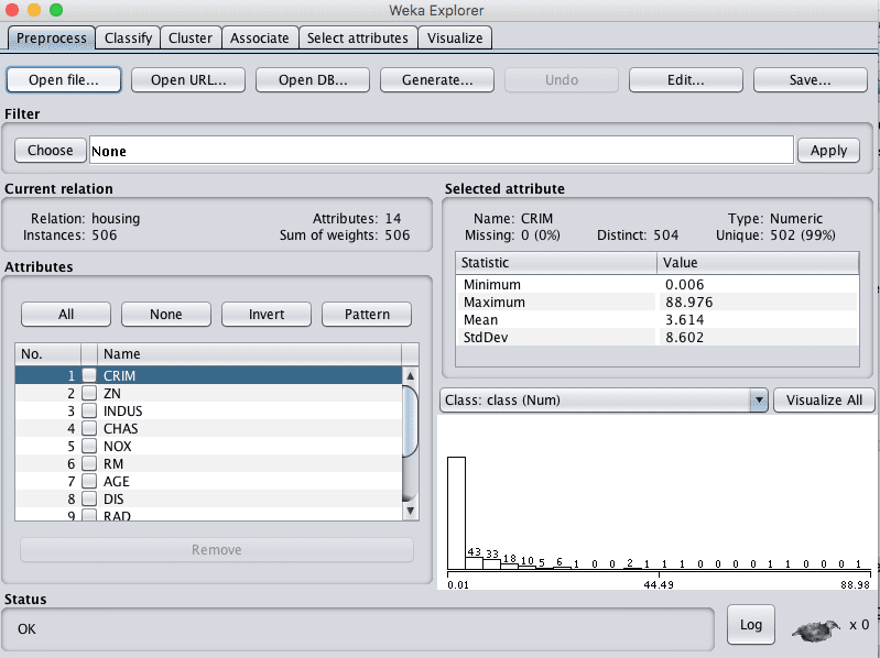
Click on each attribute in the “Attributes” pane and review the summary statistics in the “Selected attribute” pane.
We can notice a few facts about our data:
There are no missing values for any of the attributes.
All inputs are numeric except one binary attribute, and have values in differing ranges.
The last attribute is the output variable called class, it is numeric.
We may see some benefit from either normalizing or standardizing the data.
Attribute Distributions
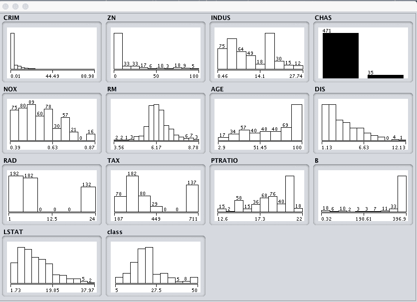
Click the “Visualize All” button and lets review the graphical distribution of each attribute.
Weka Boston House Price Univariate Attribute Distributions
We can notice a few things about the shape of the data:
We can see that the attributes have a range of differing distributions.
The CHAS attribute looks like a binary distribution (two values).
The RM attribute looks like it has a Gaussian distribution.
We may see more benefit in using nonlinear regression methods like decision trees and such, than using linear regression methods like linear regression.
Attribute Interactions
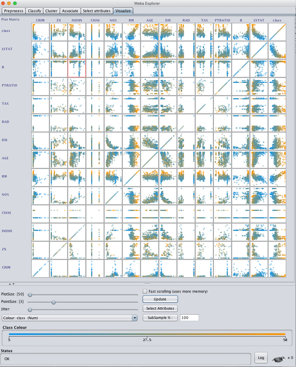
Click the “Visualize” tab and lets review some interactions between the attributes.
Decrease the “PlotSize” to 50 and adjust the window size so all plots are visible.
Increase the “PointSize” to 3 to make the dots easier to see.
Click the “Update” button to apply the changes.
Weka Boston House Price Scatterplot Matrix
Looking across the graphs we can see some structured relationships that may aid in modeling such as DIS vs NOX and AGE vs NOX.
We can also see some structure relationships between input attributes and the output attribute such as LSTAT and CLASS and RM and CLASS.
3. Prepare Views of the Dataset
In this section we will create some different views of the data, so that when we evaluate algorithms in the next section we can get an idea of the views that are generally better at exposing the structure of the regression problem to the models.
We are first going to create a modified copy of the original housing.arff data file, then make 3 additional transforms of the data. We will create each view of the dataset from our modified copy of the original and save it to a new file for later use in our experiments.
Modified Copy
The CHAS attribute is nominal (binary) with the values “0” and “1”.
We want to make a copy of the original housing.arff data file and change CHAS to a numeric attribute so that all input attributes are numeric. This will help with transforming and modeling the dataset.
Locate the housing.arff dataset and create a copy of it in the same directory called housing-numeric.arff.
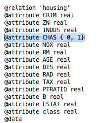
Open this modified file housing-numeric.arff in a text editor and scroll down to where the attributes are defined, specifically the CHAS attribute on line 56.
Weka Boston House Price Attribute Data Types
Change the definition of the CHAS attribute from:
1
@attribute CHAS { 0, 1}
to
1
@attribute CHAS real
The CHAS attribute is now numeric rather than nominal. This modified copy of the dataset housing-numeric.arff will now be used as the baseline dataset.
Weka Boston House Price Dataset With Numeric Data Types
Normalized Dataset
The first view we will create is of all the input attributes normalized to the range 0 to 1. This may benefit multiple algorithms that can be influenced by the scale of the attributes, like regression and instance based methods.
Open the Weka Explorer.
Open the modified numeric dataset housing-numeric.arff.
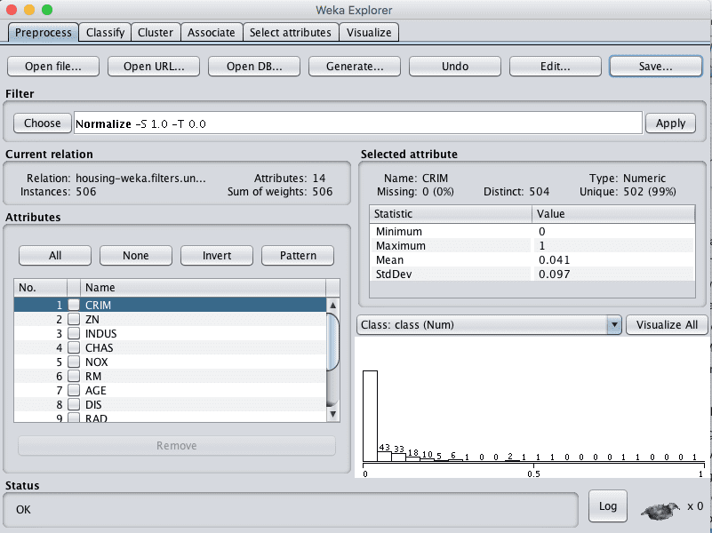
Click the “Choose” button in the “Filter” pane and choose the “unsupervised.attribute.Normalize” filter.
Click the “Apply” button to apply the filter.
Click each attribute in the “Attributes” pane and review the min and max values in the “Selected attribute” pane to confirm they are 0 and 1.
Click the “Save…” button, navigate to a suitable directory and type in a suitable name for this transformed dataset, such as “housing-normalize.arff“.
Close the Explorer interface.
Weka Boston House Price Dataset Normalize Data Filter
Standardized Dataset
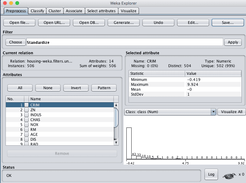
We noted in the previous section that some of the attribute have a Gaussian-like distribution. We can rescale the data and take this distribution into account by using a standardizing filter.
This will create a copy of the dataset where each attribute has a mean value of 0 and a standard deviation (mean variance) of 1. This may benefit algorithms in the next section that assume a Gaussian distribution in the input attributes, like Logistic Regression and Naive Bayes.
Open the Weka Explorer.
Open the modified numeric dataset housing-numeric.arff.
Click the “Choose” button in the “Filter” pane and choose the “unsupervised.attribute.Standardize” filter.
Click the “Apply” button to apply the filter.
Click each attribute in the “Attributes” pane and review the mean and standard deviation values in the “Selected attribute” pane to confirm they are 0 and 1 respectively.
Click the “Save…” button, navigate to a suitable directory and type in a suitable name for this transformed dataset, such as “housing-standardize.arff“.
Close the Explorer interface.
Weka Boston House Price Dataset Standardize Data Filter
Feature Selection
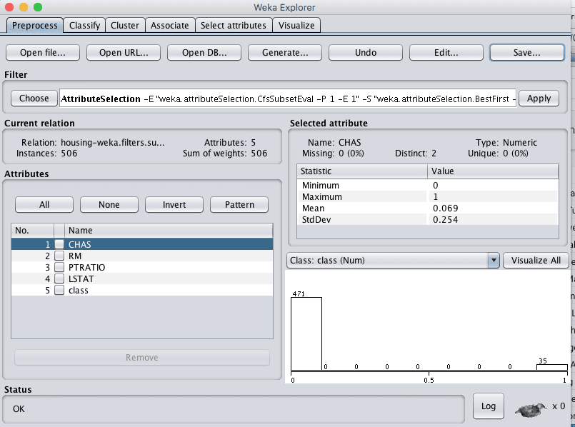
We are unsure whether all of the attributes are really needed in order to make predictions.
Here, we can use automatic feature selection to select only those most relevant attributes in the dataset.
Open the Weka Explorer.
Open the modified numeric dataset housing-numeric.arff.
Click the “Choose” button in the “Filter” pane and choose the “supervised.attribute.AttributeSelection” filter.
Click the “Apply” button to apply the filter.
Click each attribute in the “Attributes” pane and review the 5 chosen attributes.
Click the “Save…” button, navigate to a suitable directory and type in a suitable name for this transformed dataset, such as “housing-feature-selection.arff“.
Close the Explorer interface.
Weka Boston House Price Dataset Feature Selection Data Filter
4. Evaluate Algorithms
Let’s design an experiment to evaluate a suite of standard classification algorithms on the different views of the problem that we created.
1. Click the “Experimenter” button on the Weka GUI Chooser to launch the Weka Experiment Environment.
2. Click “New” to start a new experiment.
3. In the “Experiment Type” pane change the problem type from “Classification” to “Regression”.
4. In the “Datasets” pane click “Add new…” and select the following 4 datasets:
housing-numeric.arff
housing-normalized.arff
housing-standardized.arff
housing-feature-selection.arff
5. In the “Algorithms” pane click “Add new…” and add the following 8 multi-class classification algorithms:
rules.ZeroR
bayes.SimpleLinearRegression
functions.SMOreg
lazy.IBk
trees.REPTree
6. Select IBK in the list of algorithms and click the “Edit selected…” button.
7. Change “KNN” from “1” to “3” and click the “OK” button to save the settings.
Weka Boston House Price Algorithm Comparison Experiment Design
8. Click on “Run” to open the Run tab and click the “Start” button to run the experiment. The experiment should complete in just a few seconds.
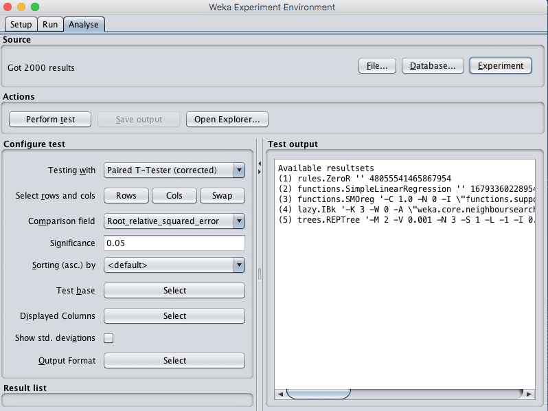
9. Click on the “Analyse” to open the Analyse tab. Click the “Experiment” button to load the results from the experiment.
Weka Boston House Price Dataset Load Algorithm Comparison Experiment Results
10. Change the “Comparison field” to “Root_mean_squared_error”.
11. Click the the “Perform test” button to perform a pairwise test comparing all of the results to the results for ZeroR.
Firstly, we can see that all of the algorithms are better than the baseline skill of ZeroR and that the difference is significant (a little “*” next to each score). We can also see that there does not appear to be much benefit across the evaluated algorithms from standardizing or normalizing the data.
It does look like we may see a small improvement from the selecting less features view of the dataset, at least for IBk.
Finally, it looks like the IBk (KNN) may have the lowest error. Let’s investigate further.
12. Click the “Select” button for the “Test base” and choose the lazy.IBk algorithm as the new test base.
13. Click the “Perform test” button to rerun the analysis.
We can see that it does look there is a difference between IBk and the other algorithms is significant, except when comparing to the REPTree algorithm and SMOreg. Both the IBk and SMOreg algorithms are non-linear regression algorithms that can be further tuned, something we can look at in the next section.
5. Tune Algorithm Performance
Two algorithms were identified in the previous section as performing well on the problem and good candidates for further tuning: k-nearest neighbors (IBk) and Support Vector Regression (SMOreg).
In this section we will design experiments to tune both of these algorithms and see if we can further decrease the root mean squared error.
We will use the baseline housing-numeric.arff dataset for these experiments as there did not appear to be a large performance difference between using this variation of the dataset and the other views.
Tune k-Nearest Neighbors
In this section we will tune the IBk algorithm. Specifically, we will investigate using different values for the k parameter.
1. Open the Weka Experiment Environment interface.
2. Click “New” to start a new experiment.
3. In the “Experiment Type” pane change the problem type from “Classification” to “Regression”.
4. In the “Datasets” pane add the housing-numeric.arff dataset.
5. In the “Algorithms” pane the lazy.IBk algorithm and set the value of the “K” parameter to 1 (the default). Repeat this process and add the following additional configurations for the IBk algorithms:
lazy.IBk with K=3
lazy.IBk with K=5
lazy.IBk with K=7
lazy.IBk with K=9
Weka Boston House Price Dataset Tune k-Nearest Neighbors Algorithm
6. Click on “Run” to open the Run tab and click the “Start” button to run the experiment. The experiment should complete in just a few seconds.
7. Click on the “Analyse” to open the Analyse tab. Click the “Experiment” button to load the results from the experiment.
8. Change the “Comparison field” to “Root_mean_squared_error”.
9. Click the the “Perform test” button to perform a pair-wise test.
(1) lazy.IBk '-K 1 -W 0 -A \"weka.core.neighboursearch.LinearNNSearch -A \\\"weka.core.EuclideanDistance -R first-last\\\"\"' -3080186098777067172
(2) lazy.IBk '-K 3 -W 0 -A \"weka.core.neighboursearch.LinearNNSearch -A \\\"weka.core.EuclideanDistance -R first-last\\\"\"' -3080186098777067172
(3) lazy.IBk '-K 5 -W 0 -A \"weka.core.neighboursearch.LinearNNSearch -A \\\"weka.core.EuclideanDistance -R first-last\\\"\"' -3080186098777067172
(4) lazy.IBk '-K 7 -W 0 -A \"weka.core.neighboursearch.LinearNNSearch -A \\\"weka.core.EuclideanDistance -R first-last\\\"\"' -3080186098777067172
(5) lazy.IBk '-K 9 -W 0 -A \"weka.core.neighboursearch.LinearNNSearch -A \\\"weka.core.EuclideanDistance -R first-last\\\"\"' -3080186098777067172
We can see that K=3 is significantly different and better than all the other configurations except K=1. We learned that we can cannot trivially get a significant lift in performance by tuning k of IBk.
Further tuning may look at using different distance measures or tuning IBk parameters using different views of the dataset, such as the view with selected features.
Tune Support Vector Machines
In this section we will tune the SMOreg algorithm. Specifically, we will investigate using different values for the “exponent” parameter for the Polynomial kernel.
1. Open the Weka Experiment Environment interface.
2. Click “New” to start a new experiment.
3. In the “Experiment Type” pane change the problem type from “Classification” to “Regression”.
4. In the “Datasets” pane add the housing-numeric.arff dataset.
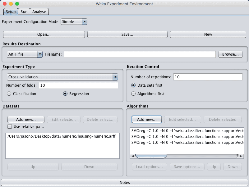
5. In the “Algorithms” pane the functions.SMOreg algorithm and set the value of the “exponent” parameter of the Polynomial kernel to 1 (the default). Repeat this process and add the following additional configurations for the SMOreg algorithms:
functions.SMOreg, kernel=Polynomial, exponent=2
functions.SMOreg, kernel=Polynomial, exponent=3
Weka Boston House Price Dataset Tune the Support Vector Regression Algorithm
6. Click on “Run” to open the Run tab and click the “Start” button to run the experiment. The experiment should complete in a about 10 minutes, depending on the speed of your system.
7. Click on the “Analyse” to open the Analyse tab. Click the “Experiment” button to load the results from the experiment.
8. Change the “Comparison field” to “Root_mean_squared_error”.
9. Click the the “Perform test” button to perform a pairwise test.
The results with the exponent=3 are statistically significantly better than exponent=1, but not exponent=2. Either could be chosen although the lower complexity exponent=2 may be faster and less fragile.
6. Evaluate Ensemble Algorithms
In the section on evaluating algorithms, we noticed that the REPtree also achieved good results, not statistically significantly different from IBk or SMOreg. In this section we consider ensemble varieties of regression trees using bagging.
As with the previous section on algorithm tuning, we will use the numeric copy of the housing dataset.
1. Open the Weka Experiment Environment interface.
2. Click “New” to start a new experiment.
3. In the “Experiment Type” pane change the problem type from “Classification” to “Regression”.
4. In the “Datasets” pane add the housing-numeric.arff dataset.
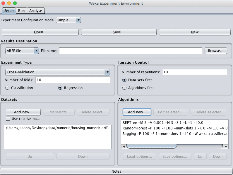
5. In the “Algorithms” pane add the following algorithms:
trees.REPTree
trees.RandomForest
meta.Bagging
Weka Boston House Price Dataset Ensemble Experiment Design
6. Click on “Run” to open the Run tab and click the “Start” button to run the experiment. The experiment should complete in just a few seconds.
7. Click on the “Analyse” to open the Analyse tab. Click the “Experiment” button to load the results from the experiment.
8. Change the “Comparison field” to “Root_mean_squared_error”.
9. Click the the “Perform test” button to perform a pairwise test.
This is very encouraging, the result for RandomForest is the best we have seen on this problem so far and the difference is statistically significant when compared to Bagging and REPtree.
To wrap this up, let’s choose RandomForest as the preferred model for this problem.
We could perform model selection and evaluate whether the difference in performance of RandomForest is statistically significant when compared to IBk with K=1 and SMOreg with exponent=3. This is left as an exercise for the reader.
11. Check “Show std. deviations” to show standard deviations of the results..
12. Click the “Select” button for “Displayed Columns” and choose “trees.RandomForest”, click “Select” to accept the selection. This will just show the results for the Random Forest algorithm.
13. Click “Perform test” to re-run the analysis.
We now have a final result we can use to describe our model.
We can see that the estimated error of the model on unseen data is 3.14 (thousands of dollars) with a standard deviation of 0.64.
7. Finalize Model and Present Results
We can create a final version of our model trained on all of the training data and save it to file.
Open the Weka Explorer and load the housing-numeric.arff dataset.
Click on the Classify.
Select the trees.RandomForest algorithm.
Change the “Test options” from “Cross Validation” to “Use training set”.
Click the “Start” button to create the final model.
Right click on the result item in the “Result list” and select “Save model”. Select a suitable location and type in a suitable name, such as “housing-randomforest” for your model.
This model can then be loaded at a later time and used to make predictions on new data.
We can use the mean and standard deviation of the model accuracy collected in the last section to help quantify the expected variability in the estimated accuracy of the model on unseen data.
We can generally expect that the performance of the model on unseen data will be 3.14 plus or minus (2 * 0.64) or 1.28. We can restate this as the model will have an error between 1.86 and 4.42 in thousands of dollars.
Summary
In this post you discovered how to work through a regression machine learning problem using the Weka machine learning workbench.
Specifically, you learned.
How to load, analysis and prepare views of your dataset in Weka.
How to evaluate a suite of regression machine learning algorithms using the Weka Experimenter.
How to tune well performing models and investigate related ensemble methods in order to lift performance.
Do you have any questions about working through regression machine learning problems in Weka or about this post? Ask your questions in the comments below and I will do my best to answer them.
HI. Thanks for the tutorial. For info there is a slight error in point 5 where not all listed are valid for regression – I see you proceed with other algorithms…:
“. In the “Algorithms” pane click “Add new…” and add the following 8 multi-class classification algorithms:
I have a question when I used any classifier with 10 fold validation for my regression problem I had a very low error but the correlation coefficient is negative do I have to test the data again using the same training set? what weka dose to calculate the correlation?
Many thanks
Afnan
Now I get the message
10:06:35: Started
10:06:37: weka.classifiers.functions.SMO: Cannot handle numeric class!
10:06:37: Interrupted
10:06:37: There was 1 error
I cannot access to house database in UCI Machine Learning Repository. Please help share this data (house.arff) here one more time to let me have a chance to practice with your awesome post.
Thank you, Why many will not prefer WEKA instead they work with Scikit for Machine Learning. Are there any advantages and disadvantages working with Weka.
Weka allows you to work through a predictive modeling problem without writing a line of code. This is a large benefit for those practitioners you do not want to code or cannot code.
Thank you very much, the tutorial helped me well, but I am confused with the predicted price, how can I know the predicted price of the house, thank you.


HI. Thanks for the tutorial. For info there is a slight error in point 5 where not all listed are valid for regression – I see you proceed with other algorithms…:
“. In the “Algorithms” pane click “Add new…” and add the following 8 multi-class classification algorithms:
rules.ZeroR
bayes.SimpleLinearRegression
functions.Logistic
functions.SMOreg
lazy.IBk
trees.REPTree
“
Thanks Mark. Updated. Logistic should not have been listed.
The normalized dataset clearly performed well for me after first iteration only. I don’t know why its same for you in all the datasets.
Dataset (1) rules.Z | (2) func (3) func (4) lazy (5) tree
—————————————————————————
housing (100) 9.11 | 6.22 * 4.95 * 4.41 * 4.64 *
‘housing-weka.filters.sup(100) 9.11 | 6.22 * 5.19 * 4.27 * 4.64 *
housing-weka.filters.unsu(100) 9.11 | 6.22 * 4.95 * 4.41 * 4.64 *
housing-weka.filters.unsu(100) 0.20 | 0.14 * 0.11 * 0.10 * 0.10 *
—————————————————————————
(v/ /*) | (0/0/4) (0/0/4) (0/0/4) (0/0/4)
Thanks for sharing your results Nilesh.
Hello Jason,
thank you for your post
I have a question when I used any classifier with 10 fold validation for my regression problem I had a very low error but the correlation coefficient is negative do I have to test the data again using the same training set? what weka dose to calculate the correlation?
Many thanks
Afnan
Are you saying that the correlation between test and train scores is negatively correlated?
Wow, I have not seen that before. Sorry. Perhaps try posting to the weka list?
I keep getting the same result in the Experimenter Run Start function
07:12:35: Started
07:12:35: Class attribute is not nominal!
07:12:35: Interrupted
07:12:35: There was 1 error
Also there is no bayes.SimpleLinearRegression. It is included under function. Is this correct?
Why do I keep getting this error.
You must change the problem type from classification to regression in the experimenter.
Now I get the message
10:06:35: Started
10:06:37: weka.classifiers.functions.SMO: Cannot handle numeric class!
10:06:37: Interrupted
10:06:37: There was 1 error
what did I do wrong now.
Thnaks
You cannot use SMO for regression.
Sorry Jason, that was my error. I was not using SMOreg and using SMO
My apologies.
Thanks
Ken
No problem.
Everything is working once I checked the Regression button.
Thanks for the help. Great tool for learning Machine Learning.
Ken
Glad to hear it.
How you calculate performances on unseen data? Why is formula 3.14 plus or minus (2 * 0.64)? I hope you understand me
You cannot.
We estimate performance of a model on unseen data using data where we know the output values.
I can solve regression problem with more than attribute for example x y have several attribute. I can build my model based on 2 attibulte field
Regression with multiple outputs? I’m not sure weka supports this sorry.
I cannot access to house database in UCI Machine Learning Repository. Please help share this data (house.arff) here one more time to let me have a chance to practice with your awesome post.
You can download it from here:
https://github.com/jbrownlee/Datasets
Hello Jason,
Thank you a lot for your precious tutorials
But unfortunately I still have ambiguities with categorical features in data sets. How can I manage them in a regression problem?
You can encode them as integers or as binary vectors.
I have examples in tutorials and Weka makes it easy.
Thank you, Why many will not prefer WEKA instead they work with Scikit for Machine Learning. Are there any advantages and disadvantages working with Weka.
Weka allows you to work through a predictive modeling problem without writing a line of code. This is a large benefit for those practitioners you do not want to code or cannot code.
Thank you very much, the tutorial helped me well, but I am confused with the predicted price, how can I know the predicted price of the house, thank you.
The predicted price is in the unit of thousands of dollars.