5 Step Life-Cycle for Neural Network Models in Keras

Deep learning neural networks are very easy to create and evaluate in Python with Keras, but you must follow a strict model life-cycle.

In this post you will discover the step-by-step life-cycle for creating, training and evaluating deep learning neural networks in Keras and how to make predictions with a trained model.

After reading this post you will know:

• How to define, compile, fit and evaluate a deep learning neural network in Keras.
• How to select standard defaults for regression and classification predictive modeling problems.
• How to tie it all together to develop and run your first Multilayer Perceptron network in Keras.

Kick-start your project with my new book Deep Learning With Python, including step-by-step tutorials and the Python source code files for all examples.

Let’s get started.

• Update Mar/2017: Updated example for Keras 2.0.2, TensorFlow 1.0.1 and Theano 0.9.0.
• Update Mar/2018: Added alternate link to download the dataset as the original appears to have been taken down.

Deep Learning Neural Network Life-Cycle in Keras
Photo by Martin Stitchener, some rights reserved.

Overview

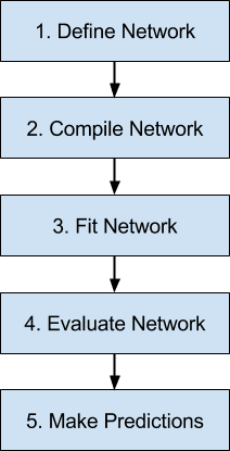
Below is an overview of the 5 steps in the neural network model life-cycle in Keras that we are going to look at.

1. Define Network.
2. Compile Network.
3. Fit Network.
4. Evaluate Network.
5. Make Predictions.

5 Step Life-Cycle for Neural Network Models in Keras

Step 1. Define Network

The first step is to define your neural network.

Neural networks are defined in Keras as a sequence of layers. The container for these layers is the Sequential class.

The first step is to create an instance of the Sequential class. Then you can create your layers and add them in the order that they should be connected.

For example, we can do this in two steps:

But we can also do this in one step by creating an array of layers and passing it to the constructor of the Sequential.

The first layer in the network must define the number of inputs to expect. The way that this is specified can differ depending on the network type, but for a Multilayer Perceptron model this is specified by the input_dim attribute.

For example, a small Multilayer Perceptron model with 2 inputs in the visible layer, 5 neurons in the hidden layer and one neuron in the output layer can be defined as:

Think of a Sequential model as a pipeline with your raw data fed in at the bottom and predictions that come out at the top.

This is a helpful conception in Keras as concerns that were traditionally associated with a layer can also be split out and added as separate layers, clearly showing their role in the transform of data from input to prediction. For example, activation functions that transform a summed signal from each neuron in a layer can be extracted and added to the Sequential as a layer-like object called Activation.

The choice of activation function is most important for the output layer as it will define the format that predictions will take.

For example, below are some common predictive modeling problem types and the structure and standard activation function that you can use in the output layer:

• Regression: Linear activation function or ‘linear’ and the number of neurons matching the number of outputs.
• Binary Classification (2 class): Logistic activation function or ‘sigmoid’ and one neuron the output layer.
• Multiclass Classification (>2 class): Softmax activation function or ‘softmax’ and one output neuron per class value, assuming a one-hot encoded output pattern.

Step 2. Compile Network

Once we have defined our network, we must compile it.

Compilation is an efficiency step. It transforms the simple sequence of layers that we defined into a highly efficient series of matrix transforms in a format intended to be executed on your GPU or CPU, depending on how Keras is configured.

Think of compilation as a precompute step for your network.

Compilation is always required after defining a model. This includes both before training it using an optimization scheme as well as loading a set of pre-trained weights from a save file. The reason is that the compilation step prepares an efficient representation of the network that is also required to make predictions on your hardware.

Compilation requires a number of parameters to be specified, specifically tailored to training your network. Specifically the optimization algorithm to use to train the network and the loss function used to evaluate the network that is minimized by the optimization algorithm.

For example, below is a case of compiling a defined model and specifying the stochastic gradient descent (sgd) optimization algorithm and the mean squared error (mse) loss function, intended for a regression type problem.

The type of predictive modeling problem imposes constraints on the type of loss function that can be used.

For example, below are some standard loss functions for different predictive model types:

• Regression: Mean Squared Error or ‘mse‘.
• Binary Classification (2 class): Logarithmic Loss, also called cross entropy or ‘binary_crossentropy‘.
• Multiclass Classification (>2 class): Multiclass Logarithmic Loss or ‘categorical_crossentropy‘.

You can review the suite of loss functions supported by Keras.

The most common optimization algorithm is stochastic gradient descent, but Keras also supports a suite of other state of the art optimization algorithms.

Perhaps the most commonly used optimization algorithms because of their generally better performance are:

• Stochastic Gradient Descent or ‘sgd‘ that requires the tuning of a learning rate and momentum.
• ADAM or ‘adam‘ that requires the tuning of learning rate.
• RMSprop or ‘rmsprop‘ that requires the tuning of learning rate.

Finally, you can also specify metrics to collect while fitting your model in addition to the loss function. Generally, the most useful additional metric to collect is accuracy for classification problems. The metrics to collect are specified by name in an array.

For example:

Step 3. Fit Network

Once the network is compiled, it can be fit, which means adapt the weights on a training dataset.

Fitting the network requires the training data to be specified, both a matrix of input patterns X and an array of matching output patterns y.

The network is trained using the backpropagation algorithm and optimized according to the optimization algorithm and loss function specified when compiling the model.

The backpropagation algorithm requires that the network be trained for a specified number of epochs or exposures to the training dataset.

Each epoch can be partitioned into groups of input-output pattern pairs called batches. This define the number of patterns that the network is exposed to before the weights are updated within an epoch. It is also an efficiency optimization, ensuring that not too many input patterns are loaded into memory at a time.

A minimal example of fitting a network is as follows:

Once fit, a history object is returned that provides a summary of the performance of the model during training. This includes both the loss and any additional metrics specified when compiling the model, recorded each epoch.

Step 4. Evaluate Network

Once the network is trained, it can be evaluated.

The network can be evaluated on the training data, but this will not provide a useful indication of the performance of the network as a predictive model, as it has seen all of this data before.

We can evaluate the performance of the network on a separate dataset, unseen during testing. This will provide an estimate of the performance of the network at making predictions for unseen data in the future.

The model evaluates the loss across all of the test patterns, as well as any other metrics specified when the model was compiled, like classification accuracy. A list of evaluation metrics is returned.

For example, for a model compiled with the accuracy metric, we could evaluate it on a new dataset as follows:

Step 5. Make Predictions

Finally, once we are satisfied with the performance of our fit model, we can use it to make predictions on new data.

This is as easy as calling the predict() function on the model with an array of new input patterns.

For example:

The predictions will be returned in the format provided by the output layer of the network.

In the case of a regression problem, these predictions may be in the format of the problem directly, provided by a linear activation function.

For a binary classification problem, the predictions may be an array of probabilities for the first class that can be converted to a 1 or 0 by rounding.

For a multiclass classification problem, the results may be in the form of an array of probabilities (assuming a one hot encoded output variable) that may need to be converted to a single class output prediction using the argmax function.

End-to-End Worked Example

Let’s tie all of this together with a small worked example.

This example will use the Pima Indians onset of diabetes binary classification problem.

Download the dataset and save it to your current working directory.

• Dataset File.
• Dataset Details.

The problem has 8 input variables and a single output class variable with the integer values 0 and 1.

We will construct a Multilayer Perceptron neural network with a 8 inputs in the visible layer, 12 neurons in the hidden layer with a rectifier activation function and 1 neuron in the output layer with a sigmoid activation function.

We will train the network for 100 epochs with a batch size of 10, optimized using the ADAM optimization algorithm and the logarithmic loss function.

Once fit, we will evaluate the model on the training data and then make standalone predictions for the training data. This is for brevity, normally we would evaluate the model on a separate test dataset and make predictions for new data.

The complete code listing is provided below.

Running this example produces the following output:

Note: Your results may vary given the stochastic nature of the algorithm or evaluation procedure, or differences in numerical precision. Consider running the example a few times and compare the average outcome.

Summary

In this post you discovered the 5-step life-cycle of a deep learning neural network using the Keras library.

Specifically, you learned:

• How to define, compile, fit, evaluate and make predictions for a neural network in Keras.
• How to select activation functions and output layer configurations for classification and regression problems.
• How to develop and run your first Multilayer Perceptron model in Keras.

Do you have any questions about neural network models in Keras or about this post? Ask your questions in the comments and I will do my best to answer them.