Do you want to do machine learning using R, but you’re having trouble getting started?
In this post you will complete your first machine learning project using R.
In this step-by-step tutorial you will:
Download and install R and get the most useful package for machine learning in R.
Load a dataset and understand it’s structure using statistical summaries and data visualization.
Create 5 machine learning models, pick the best and build confidence that the accuracy is reliable.
If you are a machine learning beginner and looking to finally get started using R, this tutorial was designed for you.
Kick-start your project with my new book Machine Learning Mastery With R, including step-by-step tutorials and the R source code files for all examples.
Let’s get started!
Your First Machine Learning Project in R Step-by-Step Photo by Henry Burrows, some rights reserved.
How Do You Start Machine Learning in R?
The best way to learn machine learning is by designing and completing small projects.
R Can Be Intimidating When Getting Started
R provides a scripting language with an odd syntax. There are also hundreds of packages and thousands of functions to choose from, providing multiple ways to do each task. It can feel overwhelming.
The best way to get started using R for machine learning is to complete a project.
It will force you to install and start R (at the very least).
It will given you a bird’s eye view of how to step through a small project.
It will give you confidence, maybe to go on to your own small projects.
Beginners Need A Small End-to-End Project
Books and courses are frustrating. They give you lots of recipes and snippets, but you never get to see how they all fit together.
When you are applying machine learning to your own datasets, you are working on a project.
The process of a machine learning project may not be linear, but there are a number of well-known steps:
Define Problem.
Prepare Data.
Evaluate Algorithms.
Improve Results.
Present Results.
For more information on the steps in a machine learning project see this checklist and more on the process.
The best way to really come to terms with a new platform or tool is to work through a machine learning project end-to-end and cover the key steps. Namely, from loading data, summarizing your data, evaluating algorithms and making some predictions.
If you can do that, you have a template that you can use on dataset after dataset. You can fill in the gaps such as further data preparation and improving result tasks later, once you have more confidence.
Hello World of Machine Learning
The best small project to start with on a new tool is the classification of iris flowers (e.g. the iris dataset).
This is a good project because it is so well understood.
Attributes are numeric so you have to figure out how to load and handle data.
It is a classification problem, allowing you to practice with perhaps an easier type of supervised learning algorithms.
It is a mutli-class classification problem (multi-nominal) that may require some specialized handling.
It only has 4 attribute and 150 rows, meaning it is small and easily fits into memory (and a screen or A4 page).
All of the numeric attributes are in the same units and the same scale not requiring any special scaling or transforms to get started.
Let’s get started with your hello world machine learning project in R.
Need more Help with R for Machine Learning?
Take my free 14-day email course and discover how to use R on your project (with sample code).
Click to sign-up and also get a free PDF Ebook version of the course.
Machine Learning in R: Step-By-Step Tutorial (start here)
In this section we are going to work through a small machine learning project end-to-end.
Here is an overview what we are going to cover:
Installing the R platform.
Loading the dataset.
Summarizing the dataset.
Visualizing the dataset.
Evaluating some algorithms.
Making some predictions.
Take your time. Work through each step.
Try to type in the commands yourself or copy-and-paste the commands to speed things up.
Any questions, please leave a comment at the bottom of the post.
1. Downloading Installing and Starting R
Get the R platform installed on your system if it is not already.
UPDATE: This tutorial was written and tested with R version 3.2.3. It is recommend that you use this version of R or higher.
I do not want to cover this in great detail, because others already have. This is already pretty straight forward, especially if you are a developer. If you do need help, ask a question in the comments.
When you click the download link, you will have to choose a mirror. You can then choose R for your operating system, such as Windows, OS X or Linux.
1.2 Install R
R is is easy to install and I’m sure you can handle it. There are no special requirements. If you have questions or need help installing see R Installation and Administration.
1.3 Start R
You can start R from whatever menu system you use on your operating system.
For me, I prefer the command line.
Open your command line, change (or create) to your project directory and start R by typing:
1
R
You should see something like the screenshot below either in a new window or in your terminal.
R Interactive Environment
1.4 Install Packages
Install the packages we are going to use today. Packages are third party add-ons or libraries that we can use in R.
1
install.packages("caret")
UPDATE: We may need other packages, but caret should ask us if we want to load them. If you are having problems with packages, you can install the caret packages and all packages that you might need by typing:
Now, let’s load the package that we are going to use in this tutorial, the caret package.
1
library(caret)
The caret package provides a consistent interface into hundreds of machine learning algorithms and provides useful convenience methods for data visualization, data resampling, model tuning and model comparison, among other features. It’s a must have tool for machine learning projects in R.
We are going to use the iris flowers dataset. This dataset is famous because it is used as the “hello world” dataset in machine learning and statistics by pretty much everyone.
The dataset contains 150 observations of iris flowers. There are four columns of measurements of the flowers in centimeters. The fifth column is the species of the flower observed. All observed flowers belong to one of three species. You can learn more about this dataset on Wikipedia.
Here is what we are going to do in this step:
Load the iris data the easy way.
Load the iris data from CSV (optional, for purists).
Separate the data into a training dataset and a validation dataset.
Choose your preferred way to load data or try both methods.
2.1 Load Data The Easy Way
Fortunately, the R platform provides the iris dataset for us. Load the dataset as follows:
1
2
3
4
# attach the iris dataset to the environment
data(iris)
# rename the dataset
dataset<-iris
You now have the iris data loaded in R and accessible via the dataset variable.
I like to name the loaded data “dataset”. This is helpful if you want to copy-paste code between projects and the dataset always has the same name.
2.2 Load From CSV
Maybe your a purist and you want to load the data just like you would on your own machine learning project, from a CSV file.
You now have the iris data loaded in R and accessible via the dataset variable.
2.3. Create a Validation Dataset
We need to know that the model we created is any good.
Later, we will use statistical methods to estimate the accuracy of the models that we create on unseen data. We also want a more concrete estimate of the accuracy of the best model on unseen data by evaluating it on actual unseen data.
That is, we are going to hold back some data that the algorithms will not get to see and we will use this data to get a second and independent idea of how accurate the best model might actually be.
We will split the loaded dataset into two, 80% of which we will use to train our models and 20% that we will hold back as a validation dataset.
1
2
3
4
5
6
# create a list of 80% of the rows in the original dataset we can use for training
# use the remaining 80% of data to training and testing the models
dataset<-dataset[validation_index,]
You now have training data in the dataset variable and a validation set we will use later in the validation variable.
Note that we replaced our dataset variable with the 80% sample of the dataset. This was an attempt to keep the rest of the code simpler and readable.
3. Summarize Dataset
Now it is time to take a look at the data.
In this step we are going to take a look at the data a few different ways:
Dimensions of the dataset.
Types of the attributes.
Peek at the data itself.
Levels of the class attribute.
Breakdown of the instances in each class.
Statistical summary of all attributes.
Don’t worry, each look at the data is one command. These are useful commands that you can use again and again on future projects.
3.1 Dimensions of Dataset
We can get a quick idea of how many instances (rows) and how many attributes (columns) the data contains with the dim function.
1
2
# dimensions of dataset
dim(dataset)
You should see 120 instances and 5 attributes:
1
[1] 120 5
3.2 Types of Attributes
It is a good idea to get an idea of the types of the attributes. They could be doubles, integers, strings, factors and other types.
Knowing the types is important as it will give you an idea of how to better summarize the data you have and the types of transforms you might need to use to prepare the data before you model it.
1
2
# list types for each attribute
sapply(dataset,class)
You should see that all of the inputs are double and that the class value is a factor:
1
2
Sepal.Length Sepal.Width Petal.Length Petal.Width Species
"numeric" "numeric" "numeric" "numeric" "factor"
3.3 Peek at the Data
It is also always a good idea to actually eyeball your data.
1
2
# take a peek at the first 5 rows of the data
head(dataset)
You should see the first 5 rows of the data:
1
2
3
4
5
6
7
Sepal.Length Sepal.Width Petal.Length Petal.Width Species
1 5.1 3.5 1.4 0.2 setosa
2 4.9 3.0 1.4 0.2 setosa
3 4.7 3.2 1.3 0.2 setosa
5 5.0 3.6 1.4 0.2 setosa
6 5.4 3.9 1.7 0.4 setosa
7 4.6 3.4 1.4 0.3 setosa
3.4 Levels of the Class
The class variable is a factor. A factor is a class that has multiple class labels or levels. Let’s look at the levels:
1
2
# list the levels for the class
levels(dataset$Species)
Notice above how we can refer to an attribute by name as a property of the dataset. In the results we can see that the class has 3 different labels:
1
[1] "setosa" "versicolor" "virginica"
This is a multi-class or a multinomial classification problem. If there were two levels, it would be a binary classification problem.
3.5 Class Distribution
Let’s now take a look at the number of instances (rows) that belong to each class. We can view this as an absolute count and as a percentage.
We can see that each class has the same number of instances (40 or 33% of the dataset)
1
2
3
4
freq percentage
setosa 40 33.33333
versicolor 40 33.33333
virginica 40 33.33333
3.6 Statistical Summary
Now finally, we can take a look at a summary of each attribute.
This includes the mean, the min and max values as well as some percentiles (25th, 50th or media and 75th e.g. values at this points if we ordered all the values for an attribute).
1
2
# summarize attribute distributions
summary(dataset)
We can see that all of the numerical values have the same scale (centimeters) and similar ranges [0,8] centimeters.
1
2
3
4
5
6
7
Sepal.Length Sepal.Width Petal.Length Petal.Width Species
Min. :4.300 Min. :2.00 Min. :1.000 Min. :0.100 setosa :40
We now have a basic idea about the data. We need to extend that with some visualizations.
We are going to look at two types of plots:
Univariate plots to better understand each attribute.
Multivariate plots to better understand the relationships between attributes.
4.1 Univariate Plots
We start with some univariate plots, that is, plots of each individual variable.
It is helpful with visualization to have a way to refer to just the input attributes and just the output attributes. Let’s set that up and call the inputs attributes x and the output attribute (or class) y.
1
2
3
# split input and output
x<-dataset[,1:4]
y<-dataset[,5]
Given that the input variables are numeric, we can create box and whisker plots of each.
1
2
3
4
5
# boxplot for each attribute on one image
par(mfrow=c(1,4))
for(iin1:4){
boxplot(x[,i],main=names(iris)[i])
}
This gives us a much clearer idea of the distribution of the input attributes:
Box and Whisker Plots in R
We can also create a barplot of the Species class variable to get a graphical representation of the class distribution (generally uninteresting in this case because they’re even).
1
2
# barplot for class breakdown
plot(y)
This confirms what we learned in the last section, that the instances are evenly distributed across the three class:
Bar Plot of Iris Flower Species
4.2 Multivariate Plots
Now we can look at the interactions between the variables.
First let’s look at scatterplots of all pairs of attributes and color the points by class. In addition, because the scatterplots show that points for each class are generally separate, we can draw ellipses around them.
1
2
# scatterplot matrix
featurePlot(x=x,y=y,plot="ellipse")
We can see some clear relationships between the input attributes (trends) and between attributes and the class values (ellipses):
Scatterplot Matrix of Iris Data in R
We can also look at box and whisker plots of each input variable again, but this time broken down into separate plots for each class. This can help to tease out obvious linear separations between the classes.
1
2
# box and whisker plots for each attribute
featurePlot(x=x,y=y,plot="box")
This is useful to see that there are clearly different distributions of the attributes for each class value.
Box and Whisker Plot of Iris data by Class Value
Next we can get an idea of the distribution of each attribute, again like the box and whisker plots, broken down by class value. Sometimes histograms are good for this, but in this case we will use some probability density plots to give nice smooth lines for each distribution.
Like the boxplots, we can see the difference in distribution of each attribute by class value. We can also see the Gaussian-like distribution (bell curve) of each attribute.
Density Plots of Iris Data By Class Value
5. Evaluate Some Algorithms
Now it is time to create some models of the data and estimate their accuracy on unseen data.
Here is what we are going to cover in this step:
Set-up the test harness to use 10-fold cross validation.
Build 5 different models to predict species from flower measurements
Select the best model.
5.1 Test Harness
We will 10-fold crossvalidation to estimate accuracy.
This will split our dataset into 10 parts, train in 9 and test on 1 and release for all combinations of train-test splits. We will also repeat the process 3 times for each algorithm with different splits of the data into 10 groups, in an effort to get a more accurate estimate.
1
2
3
# Run algorithms using 10-fold cross validation
control<-trainControl(method="cv",number=10)
metric<-"Accuracy"
We are using the metric of “Accuracy” to evaluate models. This is a ratio of the number of correctly predicted instances in divided by the total number of instances in the dataset multiplied by 100 to give a percentage (e.g. 95% accurate). We will be using the metric variable when we run build and evaluate each model next.
5.2 Build Models
We don’t know which algorithms would be good on this problem or what configurations to use. We get an idea from the plots that some of the classes are partially linearly separable in some dimensions, so we are expecting generally good results.
Let’s evaluate 5 different algorithms:
Linear Discriminant Analysis (LDA)
Classification and Regression Trees (CART).
k-Nearest Neighbors (kNN).
Support Vector Machines (SVM) with a linear kernel.
Random Forest (RF)
This is a good mixture of simple linear (LDA), nonlinear (CART, kNN) and complex nonlinear methods (SVM, RF). We reset the random number seed before reach run to ensure that the evaluation of each algorithm is performed using exactly the same data splits. It ensures the results are directly comparable.
We can see the accuracy of each classifier and also other metrics like Kappa:
1
2
3
4
5
6
7
8
9
10
11
12
13
14
15
16
17
18
Models: lda, cart, knn, svm, rf
Number of resamples: 10
Accuracy
Min. 1st Qu. Median Mean 3rd Qu. Max. NA's
lda 0.9167 0.9375 1.0000 0.9750 1 1 0
cart 0.8333 0.9167 0.9167 0.9417 1 1 0
knn 0.8333 0.9167 1.0000 0.9583 1 1 0
svm 0.8333 0.9167 0.9167 0.9417 1 1 0
rf 0.8333 0.9167 0.9583 0.9500 1 1 0
Kappa
Min. 1st Qu. Median Mean 3rd Qu. Max. NA's
lda 0.875 0.9062 1.0000 0.9625 1 1 0
cart 0.750 0.8750 0.8750 0.9125 1 1 0
knn 0.750 0.8750 1.0000 0.9375 1 1 0
svm 0.750 0.8750 0.8750 0.9125 1 1 0
rf 0.750 0.8750 0.9375 0.9250 1 1 0
We can also create a plot of the model evaluation results and compare the spread and the mean accuracy of each model. There is a population of accuracy measures for each algorithm because each algorithm was evaluated 10 times (10 fold cross validation).
1
2
# compare accuracy of models
dotplot(results)
We can see that the most accurate model in this case was LDA:
Comparison of Machine Learning Algorithms on Iris Dataset in R
The results for just the LDA model can be summarized.
1
2
# summarize Best Model
print(fit.lda)
This gives a nice summary of what was used to train the model and the mean and standard deviation (SD) accuracy achieved, specifically 97.5% accuracy +/- 4%
The LDA was the most accurate model. Now we want to get an idea of the accuracy of the model on our validation set.
This will give us an independent final check on the accuracy of the best model. It is valuable to keep a validation set just in case you made a slip during such as overfitting to the training set or a data leak. Both will result in an overly optimistic result.
We can run the LDA model directly on the validation set and summarize the results in a confusion matrix.
1
2
3
# estimate skill of LDA on the validation dataset
predictions<-predict(fit.lda,validation)
confusionMatrix(predictions,validation$Species)
We can see that the accuracy is 100%. It was a small validation dataset (20%), but this result is within our expected margin of 97% +/-4% suggesting we may have an accurate and a reliably accurate model.
1
2
3
4
5
6
7
8
9
10
11
12
13
14
15
16
17
18
19
20
21
22
23
24
25
26
27
28
29
Confusion Matrix and Statistics
Reference
Prediction setosa versicolor virginica
setosa 10 0 0
versicolor 0 10 0
virginica 0 0 10
Overall Statistics
Accuracy : 1
95% CI : (0.8843, 1)
No Information Rate : 0.3333
P-Value [Acc > NIR] : 4.857e-15
Kappa : 1
Mcnemar's Test P-Value : NA
Statistics by Class:
Class: setosa Class: versicolor Class: virginica
Sensitivity 1.0000 1.0000 1.0000
Specificity 1.0000 1.0000 1.0000
Pos Pred Value 1.0000 1.0000 1.0000
Neg Pred Value 1.0000 1.0000 1.0000
Prevalence 0.3333 0.3333 0.3333
Detection Rate 0.3333 0.3333 0.3333
Detection Prevalence 0.3333 0.3333 0.3333
Balanced Accuracy 1.0000 1.0000 1.0000
You Can Do Machine Learning in R
Work through the tutorial above. It will take you 5-to-10 minutes, max!
You do not need to understand everything. (at least not right now) Your goal is to run through the tutorial end-to-end and get a result. You do not need to understand everything on the first pass. List down your questions as you go. Make heavy use of the ?FunctionName help syntax in R to learn about all of the functions that you’re using.
You do not need to know how the algorithms work. It is important to know about the limitations and how to configure machine learning algorithms. But learning about algorithms can come later. You need to build up this algorithm knowledge slowly over a long period of time. Today, start off by getting comfortable with the platform.
You do not need to be an R programmer. The syntax of the R language can be confusing. Just like other languages, focus on function calls (e.g. function()) and assignments (e.g. a <- “b”). This will get you most of the way. You are a developer, you know how to pick up the basics of a language real fast. Just get started and dive into the details later.
You do not need to be a machine learning expert. You can learn about the benefits and limitations of various algorithms later, and there are plenty of posts that you can read later to brush up on the steps of a machine learning project and the importance of evaluating accuracy using cross validation.
What about other steps in a machine learning project. We did not cover all of the steps in a machine learning project because this is your first project and we need to focus on the key steps. Namely, loading data, looking at the data, evaluating some algorithms and making some predictions. In later tutorials we can look at other data preparation and result improvement tasks.
Summary
In this post you discovered step-by-step how to complete your first machine learning project in R.
You discovered that completing a small end-to-end project from loading the data to making predictions is the best way to get familiar with a new platform.
Your Next Step
Do you work through the tutorial?
Work through the above tutorial.
List any questions you have.
Search or research the answers.
Remember, you can use the ?FunctionName in R to get help on any function.
Do you have a question? Post it in the comments below.
This is what I can’t stand about open-source packages like R (and Python, and LibreOffice): Nobody puts in the effort required to make sure things work properly, it’s almost impossible to duplicate working environments, and the error messages are cryptically impossible. Trying to generate the scatterplot matrix above, cutting and pasting the command into R, I got the following error message:
Error in grid.Call.graphics(L_downviewport, name$name, strict) :
Viewport ‘plot_01.panel.1.1.off.vp’ was not found
Google Search provided no help. After getting featurePlot to work with all options other than “ellipse”, finally stumbled across the solution that you needed to have the “ellipse” package installed on your system. I’m guessing that you have that as a default library on your system, so you didn’t specify it was required to use that function. But how many people reading this post will be able to figure that out?
Thanks for pointing that out Leszek. To be honest I’ve not heard of that package before. Perhaps it is installed automatically with the “caret” or “lattice” packages?
Thanks for the post. I tried Google first when I saw the error, interestingly the 5th search result is the link back to this post. 🙂 It works after installing ellipse package.
He did not have the “ellipse” package as default on his system. What he did was that he installed the “caret” package using the code he provided above:
The result was that ALL the packages that were likely to be used by the “caret” package were also installed… including the “ellipse” package. You could have avoided your frustration by simply following the instructions in the tutorial.
I would like to ask you a question, hopefully you can point me in the right direction.
Last year I bought software that develops trading systems for the stock market.
It is capable to generate thousands of trading systems in a day,
The price history can be cut in three parts: in sample, out of sample and validation.
For every trading system and every price part I have metrics like: net profit, drawdown, average trade result and so on.
I would like to use the in sample and out of sample results (metrics) to try and predict the results (metrics) in the validation period.So I can determine what trading systems perform the best accoridng to the in sample and out of sample metrics and the algorithm.
What algorithm can you advice me to use in this particular case?
And, moving on, found that there were additional packages that needed to be installed and loaded, and then wound up with an Accuracy table that didn’t get the same results as you did, despite copying and pasting all the commands exactly as written. This doesn’t give me a lot of confidence about reproducibility in R.
It is true that strictly reproducible results can be difficult in R. I find you need to sprinkle a lot of set.seed(…) calls around the place, and even then it’s difficult.
The reason why your accuracy table is not the same mainly comes from the fact that the “createDataPartition()” function chooses observations in the dataset randomly. This means that the training and validation datasets are essentially different for everybody. Consequently, the end results will be slightly different.
When i loaded the caret package using below query,
> require(caret)
Output:
Loading required package: caret
Error in loadNamespace(j <- i[[1L]], c(lib.loc, .libPaths()), versionCheck = vI[[j]]) :
there is no package called ‘pbkrtest’
In addition: Warning message:
package ‘caret’ was built under R version 3.2.3
I have assigned the iris dataset to dataset2. then i executed the below query
createDataPartition(dataset2$Species, p=0.80, list=FALSE) is not working. I am getting the error message when i execute the above query.
Error Message:
Error: could not find function "createDataPartition"
Hi,
If the R version is 3.2.1 or below the caret package may turn incompatible. I faced similar issue. After uninstalling the old version I installed R 3.2.3 which fixed the error.
Thanks for sharing this. I had to grab another package (kernlab) to run the SVM fit, but everything rolled smoothly, otherwise. Great 15min introduction!
Hello Jason, this is an interesting tutorial and getting to grips with Caret still. Qs is: in the sctarrerplot matix(which is used from caret I think) how do we know what colours corespond to which class Rgds Ajit
That is a good question. It is a good idea to add a legend to your graphs.
I did not add a legend in this case because we were not interested in which class was which only in the general separation of the classes. Type ?featurePlot to learn more about adding a legend.
Thanks Jason. But more to the point .. where in the code do you assign the legend(or does the legend get picked up automatically ie which colour to which class. If it does so implicitly, how do I know what colour coresponds to what class?
Also another question
It says “We will 10-fold cross validation to estimate accuracy. This will split our dataset into 10 parts, train in 9 and test on 1 and release for all combinations of train-test splits. We will also repeat the process 3 times for each algorithm with different splits of the data into 10 groups, in an effort to get a more accurate estimate.” Hence I should expect to see 15 steps(3 times per algorithm with different splits) but we see here 5 steps(once) where do we try the other two times? kind rgds Ajit
The repetitions should be indicated in the trainControl function. When I was reading, I though 3 was the default, but this didn’t seem to be the case according to the documentation ?trainControl
You can verify that the training takes longer and the confidence intervals of the plots are smaller, so I might be right. However, I am not absolutely sure if this is correct, because I don’t know how to visually check the folds. Also, I don’t know how to get each individual result of each cv and repetition from the fits, e.g. fit.lda.
Thanks Jason for the great tutorial. I was able to reproduce the same results by following your instructions carefully. BTW, I reviewed some of the other posts above and most of the dependencies could have been resolved by loading the library(caret) at the beginning. I did encounter one issue prior to loading the library(caret) with the Error: could not find function “createDataPartition”. This error was resolved by loading the required library(caret). This loaded other required packages.
If anyone wants more practice, I did my best to recall the code Chad Hines and I added to the tutorial so one can examine the mismatches for LDA on the training set. Thank you to Jason Brownlee for this tutorial and to Kevin Feasel and Jamie Dixon for coordinating the .NET Triangle “Introduction to R” dojo last week.
Hi Jason Brownlee,
Thanks for your tutorial. However, I have a question about featurePlot function with plot = “density ” option. I couldn’t figure out the meaning of vertical axis in these plots for each features. Why the vertical axes have values that are greater than 1 (in the case of density)
Thanks, Brownlee. I would like to know of selecting best model. Is it guaranteed that a model giving highest accuracy can give the result of highest accuracy for test data? In this example, you have selected lda as the best model comparing the accuracies of the used models. But it may not predict best during testing. So my question is: when should we select our model? After training models or testing models?
Indeed it is good post, but as it is framed in the mind for ML Learners, would have explained in details of each section much more clear, for ex, 4.1 barplot section, would have explained understand number of diagram. mere walk-through would not help anything
Excellent, thank you, managed to do this with my own dataset but struggling to plot an ROC curve after. Please can you help by posting the code to plot the ROC curve? thanks
I have just started learning R and trying to use this Tutorial to fit my Dataset into it, and had a few problems like missing packages, I did however notice that when you library(caret) it will say what is missing so it’s a simple case of install.packages(missing package displayed).
I would however like to split my dataset up a bit more, this tutorial uses
“validation_index <- createDataPartition(dataset$Species, p=0.80, list=FALSE)"
My dataset is pretty large and I would like to split it into 3 or 4, like rather than an 80/20 split I would like a 50/25/25 or a 40/30/30. As I said I'm new to R so if my way of splitting it isn't the way it should be done just tell me :).
Very Nice article. Thank you. It was a very good starter for me as a new R programmer.
But one question I have is in section 6 (“Make Predictions”).
I understand that we are predicting the accuracy of our model in that section. But can you please elaborate on how to make prediction for some new data set ? I am not clear in that prediction part.
This is very helpful. Thanks. But I have a question. In a case where I have two datasets, will name them trainingdata.csv and testdata.csv, how do I load them to R but train my algorithm on training data and test it on the data set?
I know how to load this data. My question is if I have two data sets, the training data and the test data. What functions must I use for R to recognise my training data to built the models on and test data to validate. Unlike on the Iris project where they have one data and splitted it on 80% 20%
on the iris project, am getting an error for the function to partition data. See below commands.
> #attach the iris dataset to the environment
> data(iris)
> #rename the dataset
> dataset # create a list of 80% of the rows in the original dataset we can use for training
> validation_index validation_index <- createDataPartition(dataset$Species, p=0.80, list=FALSE)
Error: could not find function "createDataParti
Great post, thanks. I got it working. But when I replaced my data with iris, I got an error:
“Metric Accuracy not applicable for regression models” for all non-linier models. Here is my data:
Thank you sir ! This is really the best tutorial . I learned a lot from it and i applied it to a different dataset . But how about comparing the models using ROC curve using the caret package ?
1) You have to install ‘ellipse” package. which is missing
install.packages(“ellipse”)
2) If you change plot=pairs, you can see output. If you want, ellipse, please install ellipse package.
this is very interesting sir, but i will like help on how to better explain the plots and what each mean especially the scatterplot. i am saying in a situation where i would have to explain to an audience
Hello Jason! Thanks for making this ML tutorial. I am having trouble in the model building part. I am getting error in “rpart”, “knn”. When I run the code for rpart, the error is “Something is wrong: all the accuracy metric values are missing:” “Error: Stopping” “In addition: There were 26 warnings (use warnings() to see them)” , however for “knn”, the last error line I am getting 50 warnings.
Also , when I run “svmRadial” , it seems to run without any problem, however when i run the code for ‘rf”, I get this
Loading required package: randomForest
randomForest 4.6-12
Type rfNews() to see new features/changes/bug fixes.
Attaching package: ‘randomForest’
The following object is masked from ‘package:dplyr’:
combine
The following object is masked from ‘package:ggplot2’:
margin
I have a Version 1.0.136 of RStudio. Your help is much appreciated!
I’m sorry to hear that. Ensure you have the latest version of R and the caret package installed. You may also want to install all recommended dependencies.
This post is exactly what I was looking for. Very well put together and I’m excited about it. I will share it with some students over at UCSF. For those reading the comments, I typed everything in manually directly from Dr. Brownlee’s scripts. You learn more that way because you’re likely to make a mistake when typing at some point.
this post helps a lot but need little more clarification about boxplot and barchart becoz i am new for ml and r.could u plz explain me…it would be more helpful for me
what does this code tell us.cant understand plz help me
par(mfrow=c(1,4))
for(i in 1:4) {
boxplot(x[,i], main=names(iris)[i])
}
par(mfrow=c(1,4)) /this code specifies the gui enable a graphical display of 1 row with 4 columns
for(i in 1:4) { / this line means for each column in columns 1:4 do the follow in { code block}
boxplot(x[,i], main = names(iris)[i) / make a boxplot of the data for the column, labeled w col name
}
Thank so much sir. This is very helpful. Sir, I have a question.
When I run LDA, SVM, RF, CART model always shows that Loading required package: MASS for LDA and so on for all methods that you mention. Although I get the results without loading specific package for each methods,but is it any problem if load the specific package or not?
And if I load the package for each methods then function will be change such as for random forest we need to call the model:- randomForest(…) with package “randomForest”.
Hi, I have installed the “caret” package. But after this when i am loading through library(caret), I am getting the below error:
Loading required package: ggplot2
Error: package or namespace load failed for ‘ggplot2’ in loadNamespace(j <- i[[1L]], c(lib.loc, .libPaths()), versionCheck = vI[[j]]):
there is no package called ‘munsell’
Error: package ‘ggplot2’ could not be loaded
The box plot shows the middle of the data. The box is the 25th to 75th percentile with a line showing the 50th percentile (median). It is a fast way to get an idea of the spread of the data.
I am new to machine learning and attempting to go through your tutorial.
I keep getting an error saying that the accuracy matrix values are missing for this line:
> predictions confusionMatrix(predictions, validation$Species)
Error in confusionMatrix(predictions, validation$Species) :
object ‘predictions’ not found
predictions confusionMatrix(predictions, validation$Species)
Error in confusionMatrix(predictions, validation$Species) :
object ‘predictions’ not found
Could anyone clarify this error ?Earlier I posted something wrong
I am beginner in this so may be the question I am going to ask wont make sense but I would request you to please answer:
So when we say lets predict something, what exactly we are predicting here ?
In case of a machine (motor, pump etc) data(current, RPM, vibration) what is that can be predicted ?
set.seed(7)
> fit.lda <- train(Species~., data = data, method = "lda", metric = metric, trControl = control)
The error i got, and also tried to install mass package but it not getting installed properly and showing the error again and again please help me sir.
ERROR:-
Loading required package: MASS
Error in unloadNamespace(package) :
namespace ‘MASS’ is imported by ‘lme4’, ‘pbkrtest’, ‘car’ so cannot be unloaded
Failed with error: ‘Package ‘MASS’ version 7.3.45 cannot be unloaded’
Error in unloadNamespace(package) :
namespace ‘MASS’ is imported by ‘lme4’, ‘pbkrtest’, ‘car’ so cannot be unloaded
Error in library(p, character.only = TRUE) :
Package ‘MASS’ version 7.3.45 cannot be unloaded
My question is regarding scaling. For some algorithms like adaboost/xgboost it is recommended to scale all the data. My question is how do I unscale the final predictions. I used the scale() function in R. The unscale() function expects the center(which could be mean/median) value of the predicted values. But my predicted values are already scaled. How can I unscale them to the appropriate predicted values. I am referring to prediction on unlabeled data set.
I have searched for this in many websites but have not found any answer.
> library(tidyverse)
Sir while adding this library in R, I have installed the package then also it is showing following the error: please help me
Error in loadNamespace(j <- i[[1L]], c(lib.loc, .libPaths()), versionCheck = vI[[j]]) :
there is no package called ‘bindrcpp’
Error: package or namespace load failed for ‘tidyverse’
Dear Jason,
I am not familiar with R tool. When I started reading this tutorial, I thought of installing R. After the installation when I typed the Rcommand, I got the following error message. Please give me the suggestion…
> install.packages(“caret”)
Installing package into ‘C:/Users/Ratna/Documents/R/win-library/3.4’
(as ‘lib’ is unspecified)
— Please select a CRAN mirror for use in this session —
trying URL ‘http://ftp.iitm.ac.in/cran/bin/windows/contrib/3.4/caret_6.0-77.zip’
Content type ‘application/zip’ length 5097236 bytes (4.9 MB)
downloaded 4.9 MB
package ‘caret’ successfully unpacked and MD5 sums checked
The downloaded binary packages are in
C:\Users\Ratna\AppData\Local\Temp\RtmpQLxeTE\downloaded_packages
>
Hi Jasson,
I tried the following but got the error,
> library(caret)
Loading required package: lattice
Loading required package: ggplot2
Error: package or namespace load failed for ‘caret’ in loadNamespace(i, c(lib.loc, .libPaths()), versionCheck = vI[[i]]):
there is no package called ‘kernlab’
>
When I created the updated ‘dataset’ in step 2.3 with the 120 observations, the dataset for some reason created 24 N/A values leaving only 96 actual observations. Copy and pasted the code from the post above. Any idea what caused or how to fix so that the ‘dataset’ is inclusive of all the training data observations? Doesn’t seem to be anything wrong with the IRIS dataset or either of the validation_index or validation datasets.
Update to OP, I reran the original commands from that section and was able to pull in all 120 observations for the training data. Not sure why it didn’t fetch all the data the first time but looks ok now.
Just confirming, the above tutorial is a multiclass problem? Therefore, I should be able to apply the above methodology to a different k=3 problem. Is this correct?
For my first Machine Learning Project, this was EXTREMELY helpful and I thank you for the tutorial. I had no problems going through the script and even applied to a dummy dataset and it worked great. So thank you.
My question is more related to automation. Instead of manually assessing the accuracy of each model to determine which one to use for prediction, is there a way to automatically call the model with the highest accuracy in the “predictions <- predict([best model], validation)" script. Hope to hear from you soon.
For learning R I strongly recommend the Coursera.org “R Programming” certification course, When I took it it was free, now is paid, something around USD 50.
successfully done, and got the result.Thanks for the great tutorial.
But now i wonder, what to do further, how to use it in a generic manner for any dataset.
How to use the created pred.model anywhere.
ohk, but to use any dataset we need to make the dataset similar to that of the iris dataset, like 4 numberic columns, and one class.
Also, accuracy output is similar over the traning dataset , and the validation dataset, but how does that help me to predict now what type of flower would be next if i provide it the similar parameters.
Now, for example i have to create a model which predicts the cpu utilization of the servers in my Vcenter or complete DC, how can i create a model which will take my continious dataset and predict that when the CPU utilization will go high and i can take proactive measures.
Thanks for the clear and set by step instructions. But I just want to understand what I need to do after creating the model and calculating its accuracy ? Can you please explain to draw some conclusions/predictions on the iris data set we used ?
Thank you very much for the tutorial I have been very useful but I have a question, in the section of “print (fit.lda)” does not deploy “Accuracy SD Kappa SD”.
What remains of the tutorial if you have given me exact, could you help me with this doubt ?.
Upon further reading of other articles written by you, I realize that I may not need to use ‘Regression’. My dataset has category variables as input and category attributes as output as well (having 7 levels). So, it is a classification problem and I’m assuming I can use one of the 5 models/fit you have given as examples here in this Iris project. Can you let me know if this is correct understanding?
– Thank you
It works for me with the iris data. Thanks a lot Jason! But there are no “Accuracy SD Kappa SD ” from the output of the fit models. Should I change some settings to get them?
Dear Jason Brownlee
I have a dataset with 36 predictors and one for classes (“1”, “2”, “3”) that I got it through clustering in the previous step.
My question is: how can I reduce all my predictors into five variables representing specific dimensions in my study?
Should I run PCA separately to produce a new dataset with 5 predictors and one for classes or is there any other ways?
Thank you in advance.
Hi Jason, I am getting the error –
Error: could not find function “trainControl”
on typing tc<-trainControl(method="cv",number=10).
What can be the solution for this?
Maybe a very stupid question. But I read “Build 5 different models to predict species from flower measurements”. So now I am wondering what the predictions of the model tell me about this, how I can use it. For example I now go to the forest take some measurements, assume that the flower is one of those tested, and want to know which flower it is exactly. In a traditional regression formula it is straightforward as you can put in your measurements in the formula and the calculated estimates and get an outcome. But I don’t know how to use the outcomes in this case.
Hi Json how are ?
I am new in machine learning. i want to invent a unique idea and prof about islami banking and conventional banking. how can i do that. if any suggestion please give me and i cant fund any islami banking data set like loan info or deposit bla bla bla. i want your valuable information
Hi Jason, First of all great work. May God bless you for all your sincere efforts in sharing the knowledge. You are making a big difference to the lives of people. Thank you for that.
I have a basic question. Now we have a best fit model – how to use it in day to day usage – is there a way I can measure the dimensions of a flower and “apply” them in some kind of equation which will give the predicted flower name? How to use the results? Kindly advise when you are free.
Hi Jason,
Thank you for sharing your methods and codes. It was very useful and easy to follow. Could you please share how to score a new dataset using one of the models? For example, in my training, random forest has the best accuracy. Now I want to apply that model on a new dataset that doesn’t have the outcome variables, and make prediction.
Thank you
Thanks Jason. I read through the link. I already finalized my model, now I need save the model and apply it for operational use. The dataset that I want to score doesn’t have the outcome variable. I am not sure which command I should use to make prediction after I have the final model. Can you suggest R codes to do so?
Hi Jason! Amazing post! I have the same doubt @TNguyen did. I Finalized the model and we know that LDA is the best model to apply in this case. How I predict the outcome variables (species) in a new dataframe without this variable? IN summary, how I deploy the model on a new dataset? Sorry, I´m new in this field and I´m learning new things all the time!
Thanks for the great tutorial. I have a problem and don’t know what’s wrong in the section
3.1 Dimensions. When I execute dim(datset) I get the answer NULL.
Do you know why R Studio doesn’t show me the dimensions of the “dataset”?
Hey, I am working on the package called polisci and I am asked to build a multiple linear regression modal. My dependent variable is human development index and my independent variable is economic freedom. Could ou please tell me how can I perform multiple linear regression modal. How do I go about in steps and what is the syntax in R to get to the results and get a graph? Any help would be greatly appreciated. Please help me as I am an undergrad student and I am learning this for the first time
Thanks, Jason! This is a very helpful post. I did exactly as suggested, but when i print(fir.lda), I do not have the accuracy SD or kappa SD. How should I get them? Thanks
Thanks for the great tutorial. I have a problem and don’t know what’s wrong in the section
6. Make predictions . When I execute predictions <- predict(fit.lda, validation)
confusionMatrix(predictions, validation$Species) I get the error "error data and reference should be factors with the same levels."like this
Do you know why R Studio doesn’t show me the Make predictions of the “dataset”?
When I try to do the featurePlots I get NULL. I installed the ellipse package without error.
featurePlot(x=x, y=y, plot=”ellipse”)
NULL
> # box and whisker plots for each attribute
> featurePlot(x=x, y=y, plot=”box”)
NULL
> # density plots for each attribute by class value
> scales featurePlot(x=x, y=y, plot=”density”, scales=scales)
NULL
Dear Dr Jason,
Two situations – (i) the NULL problem – rectified, and (ii) displaying multivariate graphs. and (iii) typo error
(i) The NULL problem rectified.
I too was getting the problem at section 4.2 on multivariate plots. The problem was fixed.
You were correct that another package you must install. That was in 2018. Referring to the 2019 Updated subheading at the top of the page, it is necessary to install other packages by typing:
The package on my internet connection took nearly 2 hours. But it was worth it.
(ii) Displaying the barplot in section 4.1 and multivariate graphs.in section 4.2
In order to get the barplot and multivariate plots in sections 4.1 and 4.2 respectively to display in the whole window, I would add this line:
1
par(mfrow=c(1,1))
Otherwise you will get the barplots and the featurePlots all squeezed in because the command
1
par(mfrow=c(1,4))
continued from section 4.1 and operated on barplots and featurePlots.
So as soon as you deal with barplots in section 4.1 put in this line
1
par(mfrow=c(1,1))
Also there is a typo error in section 4.2. Where it says
“Like he boxplots, we can see the difference in distribution of each attribute by class value. We can also see the Gaussian-like distribution (bell curve) of each attribute.”
Replace “Like he boxplots….” with “Like the boxplots….”
Great tutorial Jason! Inspired me to look up and a learn a bit more about LDA and KNN etc. which is a bonus! Great self-learning experience. I have experience with analytics but am a relative R newbie but I could understand and follow with some googling about the underlying methods and R functions.. so, thanks!
One thing… the final results comparison in Section 5.3 are different in my case and are different each time I run through it. Reason is likely that in Step 2.3 there is no set.seed() prior. So, when you create the validation dataset which is internally a random sample in createDataPartition().. results are different in the end?
# create a list of 80% of the rows in the original dataset we can use for training
validation_index <- createDataPartition(dataset$Species, p=0.80, list=FALSE)
# select 20% of the data for validation
validation <- dataset[-validation_index,]
# use the remaining 80% of data to training and testing the models
dataset <- dataset[validation_index,]
1
2
3
4
5
6
# create a list of 80% of the rows in the original dataset we can use for training
validation_index <- createDataPartition(dataset$Species, p=0.80, list=FALSE)
# select 20% of the data for validation
validation <- dataset[-validation_index,]
# use the remaining 80% of data to training and testing the models
dataset <- dataset[validation_index,]
1. install.packages(“caret”, dependencies = c(“Depends”, “Suggests”)) ran for almost an hour. May be connectivity to mirrors.
2. install.packages(“randomForest”) & library(“randomForest”) needed
Would definitely recommend this to all ML aspirants as a “hello world!”
First I’d like to say THANK YOU for making this available! It has given me the courage to pursue other ML endeavors.
The only issue I have is that when summarizing the results of the LDA model using the print(fit.lda), my results do not show standard deviation. Do you know if this is due to a setting in R that needs to be changed?
First of all great tutorial, I followed and achieved the expected results
Really helped me overcome ML jitters. Very very grateful to you.
But I really wanted to know the mathematical side of these algorithms, what do these do and how?
Also,
it would be wonderful if you could explain things like “relaxation=free” (What does this mean?) That do not have a straight answer on Google
Thanks
Regards
1. Post an unsupervised Random Forest tutorial. I think Caret only supports supervised. If not could you please point me to an example other than Breiman’s
2. More specifically I am looking for a predict program that takes a saved model eg Random Forest and loops through an input .csv file with class/Type predictions. Think I have the probability figured out
When I insert my mysql database data in the dataset and try to run the above sample, I get the error:
> validation_index <- createDataPartition(dataset$containsreason, p=0.80, list=FALSE)
Error in cut.default(y, unique(quantile(y, probs = seq(0, 1, length = groups))), :
invalid number of intervals
I tried searching but could not find any instance of this error.
this really was life saving for as it was just when i was wondering to make a structure of my exam report in climate studies. Thank You sooooooooo much
Working perfectly.Had to install many packages though.But all worked out well with some mouse clicks and with some Google. MY FIRST SUCCESSFUL MACHINE LEARNING TUTORIAL EVER!!!!! MANY THANKS JASON!!-Love and respects from India.
Dear Brownlee , first of all thanks for this wonderful tutorial.
I would like to learn that when we found the most accurate model , how can we ask to our model to test further samples , ie how can we run our test for one more sample data ?
for example in your test lda was the most accurate, so if you want to ask your program to check for another data what is the code for it?
thanks
isa
Hey Jason, I have the same question as isa, and I’ve read your post on creating a final model. How does the idea of choosing a final model and giving it unseen data to analyze translate to R code? In the code above, for instance, lets say I wanted to give one row of iris flower qualities to fit.lda and have it guess what species it was. How would I do that? Thanks for the help.
Thanks for the tutorial! I copy the code and it works fin till Predictions part. I get an error: Error in eval(predvars, data, env) : object ‘Sepal.Length’ not found. Could you please help me out? Thanks in advance!
Could you plz guide how can we get the predicted value (especially in regression) for each instance of the dataset. For instance, we have 5 variables, then how can we get the five predicted (numeric) values so that we compare these values with the actual values of the dataset.
I am an enthusiast of R language. I am a asst prof and research scholar so i am working on ML and R. The post was very useful. I already worked with different packages but this is very simple than all other. I need one small advice, how can i make R as favorite language for my b.tech students. They are strongly supporting python but i want to make same interest with R also.
Hi Jason, I’m at my wits end here. pulled all of my hair. have given up on google. searched high and low and cannot understand/get the answer to this question.
i created a model ham/spam classifier…it’s fine. but now i want to use it on a BRAND NEW data. or run 1000 rows of brand new data through it. How the heck do i do this?
i used the predict function, it works fine on the test data but on the new data (after i’ve done all the preprocessing) i get an error of object not found … object is a word and i’m assuming it doesn’t exist in one of the sets…i haven’t a clue.
so i guess i’m missing a step somewhere? please help
Hey Jason Thank u so much for this usefull post. Im’doing my postdegree project about optimize a supply chain system with AI. So I would like to ask you if the best Branch to forecast demand and optimize a process like this (Supply chain) is ML with neuronal networks. where can I find more information about your courses. Thanks again Merry Christmas
Hi Jason,
this was my first R experience and your tutorial helped me a lot.
Although, the was seems to be long.
For example: does “fit” support also other algorithms like e.g. tensor flow?
When I go into the help system I cannot find anything about the possible algorithms.
nice tutorial. All worked fine for me except when trying to fit the linear algorithm “lda”.
No matter which variables I’m using (I also tried with your example).
I get this error:
Something is wrong; all the Accuracy metric values are missing:
Accuracy Kappa
Min. : NA Min. : NA
1st Qu.: NA 1st Qu.: NA
Median : NA Median : NA
Mean :NaN Mean :NaN
3rd Qu.: NA 3rd Qu.: NA
Max. : NA Max. : NA
NA’s :1 NA’s :1
Error: Stopping
In addition: There were 11 warnings (use warnings() to see them)
Very nice tutorial!!
I was wondering: after I get a good model that can make good prediction on new datasets, how can I say which parameters are more important for the prediction? In other words, which are the important features? For example In this case I can say that I.Setosa has short sepals and short petals (etc…). But can I get the same information printed from the script?
Thanks in advance!
Perhaps try an ablative experiment, where you refit the model with each feature removed in turn, and see which feature or features negatively impacts the performance of the model the most?
Hello jason, thank you for this demo on this algorithms. The explanation was quite clear and to the point.
However, my question is, i use the above code to run a project but in the models i got some errors here is the descrription of my data..
1. i have 19 predictors and 1 response variable. but the response is categorical 1 for yes and 0 for no.. so i import the data and step by step follow your code but in the models, i use “metric = metric” but that does not work so i use “metric = Accuracy” in that as well, i got an error in using LDA, kNN and almost all the models and the error says this cannot be run on regression. but my outcome is categorical and initially i change it into factor. after all error,
2. the second part was, i now use data with 19 predictors and i use an outcome variable of 3 levels instead of 2. but this time i just maintain “metric = Accuracy” and this runs on all models without any error. the the only error results in the portion where i want to do the prediction..below is the error that result when i want to do the prediction
“Error: data and reference should be factors with the same levels.” what does this error means?
thank you and i need your response in both of my questions.
Hello Jason;
Thank you very much for the informative tutorial. I may miss some point here, each time I run the algorithm, I got different results. I mean that at one-time LDA was the most accurate model, another time kNN was and another time LDA, Cart, and rf had the same accuracy value. Surely, each time another train data set was used but the results were confusing. One thing, how can I see the coefficients of the models or can I?
Thank you in advance
Thank you, your tutorial is very useful for my work. May I ask one question, how can add lebels of each line in the plot (blue pink and green line) as their species (“setosa” “versicolor” “virginica”) in “Density Plots of Iris Data By Class Value” ?
Hi! Like others, I’m having trouble with the featureplot line. I tried updating R, and installing “ellipse” by itself and finally used the additional code for installing caret with the additional specifications. I am still getting “error in featurePlot (x=x, y=y, plot= “ellipse”) : could not find function “featurePlot”.
Thank you very much Jason! You are a great tutor. Extremely helpful. I did not manage to install the caret package in R (got some error message which I couldn’t solve) but your tutorial worked perfectly for me in RStudio.
I am italian student, i want find from these 4 classifier method ( Multinomial regression, Discriminant analysis (linear or quadratic), KNN
classifier ) the best in terms of minimum number of misclassified records and why ? with comment and consideration. The input is IRIS dataset end the goal is perform the classification of the data in terms of the attribute in
column 5, labeled “species” (with values: setosa, versicolor, and virginica),
with respect to the four measurements: “Sepal.length”, “Sepal.width”,
“Petal.length”, and “Petal.width”, presented in columns 1-4
Awesome post for R beginners like myself.
I have some questions:
1) My dataset is quite higher compared to Iris’. I have 170 columns (different variables) and 4000 rows, but around 3-8% data is missing in each column. I have found that we could either impute these missing data point with the median, mean or not include them in the analyses. I am going for the median, but is this better than no analysing them?
2) For learning purposes, I have chosen 13 columns (those virtually with no missing data) + all rows and it works fine with values around or bigger than 98%. However, when using all columns the accuracy/sensitivity, etc drops to around 60%. So, is this “Ok” if I include those variables that influence the most?
3) When a database has missing data, the box and whisker plot doesn’t come up (4.1. Univariate plots). I usually get “error in call.Graphics….” or columns not define.
Hope you can clarify this questions,
Thank you for your help.
Best regards,
Alan
Thank you for posting this fantastic tutorial. I am very new to machine learning and have a quick, and probably naive, question.
How can I see the final equation which is used to predict a classification? The iris dataset and another dataset of my own convinced me how effective this can be. I would like to know the weight of each variable in determining the predicted classification.
Hi Jason, thank you for this post! It is very helpful. I wonder if the equation cannot be seen, are there any other ways for us to see which variables are the most influential ones in the model for predicting an outcome?
Hello sir I am new to R thanks for your above first project explanation,
now my doubts,
1. my file is excel contain more than 1000 rows with nearly 20 columns (with names) last column class ( 2 classes like yes no) in other columns some collumns values are numbers and some 4 columns having string (one column values like Yes, No and another column values like 11 Place names etc.) to do above give your first R project can I apply (excel convert as) csv file or I apply after convert string column values to numeric, if yes is can I give 1,2,3,4,5,6… different places names respectively.
2. How I use these R to do my research for my above said dataset for classification or to analysis by change some thing in classification methods.
Thank you,
By
Suresh Kumar
Hi Sir!
Can You help me out, I’m working with my Final Year Project and accidentally we choose the Artificial Intelligence Project. In our project, we need to implement Artificial Neural network. It is base on student academic performance predictions, where we will predict which fields are best for the student in future studies by using their past academic data. Now even I don’t know where to get start.. remaining module of our app has been done but we are stuck in this last module. Can you help me how we should start which tools are used for code and how we will train our network depending upon student classifications? after getting training, we have to integrate it with our android studio project. Please Help!
Thanks in advance!
I’m zero in machine learning.. so please give me some time for ur kind reply.. guide me where i should start which tools should i used for it..
Thanks for the great post. I’m a beginner in this and have a couple of perhaps dumb questions:
1. For each of the 5 models, especially the random forest one, how do I find out the chosen parameters of the models? For example, for rf, which predictors are used? what are the parameters for each of the predictors to predict the results?
2. how do I know what the predictions will be for a new set of data? In other words, if we provide a new set of values for “Sepal.Length”,”Sepal.Width”,”Petal.Length”,”Petal.Width” and want to know what the model predicts the species is, how do I do that?
hi jason Brownlee..great work published by you thanx….while running the code i am facing these errors….i have copied the code plus errors here.kindly guide me whats the problem?
set.seed(7)
> fit.knn # c) advanced algorithms
> # SVM
> set.seed(7)
> fit.svm # Random Forest
> set.seed(7)
> fit.lda fit.rf <- train(Species~., data=dataset, method="rf", metric=metric)
Error in metric %in% c("RMSE", "Rsquared") : object 'metric' not found
Thanks for such a wonderful guide. Can you please explain how to interpret the scatterplot matrix? I can understand if we use it to plot the relationship between two variables. I am not able to understand the relation between 3 variables through the graph that you have plotted in this tutorial.
Do you know of a working example of the Dodger Loop Sensor problem? I am currently stuck trying to merge the two data csv’s and use the correct columns.
Using the dat from the two data file build a predictive model to predict the occurrence of a baseball game based on the loop sensor data. I am stuck trying how to clean and combine the data. It seems no one has ever tackled this problem… I am stumped. Any help would be appreciated.
Thanks for the great tutorial. Can you tell me how to display the confusion matrix for the cross-validation step (sums and/or mean)? While evaluating the 20% validation subdataset is informative, I have a very small dataset so it would be more informative if I could see the confusion matrix from the cross-validation step.
Thank you Jason, this website and it’s tutorials are fantastic! I’ve read a lot of textbooks and currently working in the field, but still feeling a bit confused until I came across your site. You make it so easy! Thank you so much.
Hi! Thanks for providing this tutorial. I am working on a project that is very similar to your example–the difference is that it is linear regression. I’m using the caret package and the train function with “full model”, “forward selection/leapForward”, and “ridge regression” and using the metric “RMSE” as the performance metric. I need to select the model with the lowest “RMSE”. I am using pretty much thes same script you are in the example. My problem is that I’m lost in the theory of what I’m doing. Here’s what I know and where I get lost:
1) created train set and test set
2) pre-processed the train set — centered, scaled, and removed non-zero variance features
3) set up the train control
4) built the 3 models
5) compared the results using “resamples”
6) picked the model with the lowest RSME (which was the forward_selection/leapForward model)
7) Used “predict” to compare the observed values to the predicted values of the forward selection
8) Finally, I created a table that shows the errors between the observed and predicted results and plotted those.
What do I do next? When using “lm”, you get a summary statistic that shows the coefficients, p value, r-squared — but how do you do this with “leapForward”?
I used “VarImp” and found that with the forward_selection model, there is only 1 feature that is highly correlated — do I then use this to run another linear regression using that 1 feature?
I’m close to understanding but not close enough to figure out what to do next…
Would very much appreciate a response to this as well, for I’m stuck on the “next” step after building the model. Can we predict completely NEW data points using this newly built model and not just use it as a comparison to train vs test data?
I have the same issue as Muriel. I did not get the caret package installed when i invoked
“install.packages(“caret”, dependencies=c(“Depends”, “Suggests”))”. Can i independently download the caret package from anywhere and install it in R?
Jason, this is a very well made tutorial. It is really helpful for me – yes, there might be some issues with additional packages, like e1071, which has to be installed on the fly in my case.
But as longer one sits with this one, the better he understands. Just have to get my hands on more projects like that.
I come from Power BI side of things, want to delve deeper into data analysis and.. yes, machine learning and AI – who knows!
Great tutorial, really appreciated.
Many thanks for your help. I have a question. After I tested the best model on the test dataset, how can I apply the model on new unlabeled data (e.g. to classify patients or healthy individuals) or to classify even a single individual (ill vs. healthy) based on data of the model?
Is there a code for this?
Many thanks
#since the input ariables are numneric we create box and whisker plots
> par(mfrow=c(1,4))
> for(i in 1:4) {
+ boxplot(x[,i], main=names(iris_train)[i])
+ }
Error in oldClass(stats) <- cl :
adding class "factor" to an invalid object
I really needed this Hello, World type of ML project. Thank you!
I studied the whole book Data Science in Business, which is great for a conceptual understanding. Their intention is explicitly not to cover algorithms. Still, a whole semester of nothing concrete failed to build my confidence.
I don’t think that was exactly a bad plan, for now when I run the algorithms I know what they are, and that’s pretty cool. Nevertheless, I really needed to run something! This did it. Yay.
Error in terms.formula(formula, data = data) :
duplicated name ‘NA’ in data frame using ‘.’
I keep getting this error . Can you please tell me how to debug this?
Couldn’t get my data to load from the start. In the beginning steps where you say you to name the file “iris.csv”, which I did but R-studio would not load anything after that. Kept on getting error messages, and could not make it through part 2.2. Please help!
Hi, This is very useful for me.
I have a doubt.
“the R platform provides the iris dataset for us”, The line given above
what is the R platform didn’t provide a particular dataset that i want to use?
So what are the steps to go with.
When I try to prediction with all base (5952 obs of 23 var=
“Error: data and reference should be factors with the same levels”
Then, I have a partition with the 20% an said:
“Error in model.frame.default(Terms, newdata, na.action = na.action, xlev = object$xlevels) factor SECTOR.ADH has new levels Sector No Definido (solo para bolsas y envoltorios)
Any idea about how to prepare data containing different scales and units (e.g., Age, Gender, Start time, Start Date, Distance, etc.) for a machine learning project.
I have just finished your ebook “Machine Learning Mastery with R” and I would like to thank you so much because I enjoyed so much the travel through the book. Excellent and impressive pragmatic work.
Hi, great content.
I have been struggling since last sunday with the rlang 0.4.6 package. When I put library(caret), the program shows:
Error: package or namespace load failed for ‘caret’ in loadNamespace(i, c(lib.loc, .libPaths()), versionCheck = vI[[i]]):
namespace ‘rlang’ 0.4.5 is already loaded, but >= 0.4.6 is required
Please, could you explain me how to overcome this problem? I already have installed the whole package with install.packages as you told above. I also tried using this link https://cran.r-project.org/web/packages/rlang/index.html but the same message is shown.
Thank you for your answer.
pd. I am using the r 4.0.0 version on win 10
Hi, again
After trying many times to run the library(caret) in R. I downloaded the rlang package in Rstudio and then all the libraries I could not run in R are available. Maybe Rstudio after restarting the program follows the right steps to install a package.
Thank you for your answer.
@luis first restart R session from R studio, which helps uload all loaded packages. Once restarted, update all packages before loading any package. The error you’re getting is because you are trying to update a package which is loaded.
I would like to ask something
What is difference between R and python?
Because in my point of view all are same with different advantages
So if there is difference what is R advantage over python .
And if they are no difference then why using R that is not as popular as python that popular will help because the more users using it the more support of those users we have like error solutions ect.
Thanks for the wonderful post Jason. I am a beginner in data science, as a matter of fact I just started few days back. I am getting very confused whenever I download a data set to practice in ‘R’. although there have been times when it took me way longer than normal just to figure out how to calculate Z-scores & T-scores using just the confidence levels. I am really clueless on the datasets that I download as there is no business problem given along with that, since its just the data sets, I usually run the plotting commands, look for missing values, look for normal distribution etc as I figured out that some datasets have nothing to do with Regressions etc. How do you suggest for a newbie to look ‘Where’ in the data set for the business problem or the purpose of the data collection. It will be of much help.
Seeking a mentor like you.
Thanks in Advance!
aahh..and yes I am for biotechnology background and have no coding experience, I look up “R in Action” and try to mimic the commands to understand the codes.
Hi Jason, thanks for a great tutorial for getting started with R and classification problems. Have worked through it and done first pass application to my own data. Question:
How can I get an indication of the quality or goodness of fit for the classification of an unknown? After all, new data may not match the model as well as the training/validation data set did. Also, new data may be for a class that was not part of the training exercise, and so you shouldn’t get a good match.
Thanks.
thank you for this great free tutorial. Please I am getting different result when I executes
“# list types for each attribute
sapply(dataset, class)”
Below is my output:
Sepal.Length Sepal.Width Petal.Length Petal.Width Species
“numeric” “numeric” “numeric” “numeric” “character”
I having “character” instead of “factor” and when I executed
# list the levels for the class
levels(dataset$Species)
the output is NULL.
Please, how can I fix this problem?
Thank you very much
Thanks for your response. However, I am using the latest version of R, I run from command line prompt, but the problem is not yet solved, instead of “factor”, I am getting “character”.
Great tutorial. I am wondering: When doing binomial predictions out of observations, how can I take into account that I care more about specificity than sensitivity? I would like to perform feature selection out of a few dozens of observations while keeping in mind that the specificity shouldn’t be lower than a certain threshold.
When I tried the plots using the data which was imported as .csv file, it gives a warning
NAs introduced by coercion
and then the plot was empty. Any suggestions for this?
Amazing issues here. I am very happy to see your article.
Thanks so much and I’m taking a look forward to contact you.
Will you kindly drop me a e-mail?
Thanks for this tutorial.
Just a question… how do I know which color matches which response category?
I borrowed this code to play with one of my own datasets but I don’t know which level blue, pink and green apply to in the featurePlots
hi,
mine none of below is working out. I wanted to know the correct value or the parameter to mention below, as lease one model if you can help with.
# a) linear algorithms
set.seed(7)
fit.lda <- train(Species~., data=dataset, method="lda", metric=metric, trControl=control)
# b) nonlinear algorithms
# CART
set.seed(7)
fit.cart <- train(Species~., data=dataset, method="rpart", metric=metric, trControl=control)
# kNN
set.seed(7)
fit.knn <- train(Species~., data=dataset, method="knn", metric=metric, trControl=control)
# c) advanced algorithms
# SVM
set.seed(7)
fit.svm <- train(Species~., data=dataset, method="svmRadial", metric=metric, trControl=control)
# Random Forest
set.seed(7)
fit.rf <- train(Species~., data=dataset, method="rf", metric=metric, trControl=control)
Thanks for the great tutorial!
Just a question… in the prediction step, are we supposed to send only the independent variables in “validation” (i.e., the x_test) instead of all the validation?
it’s not supposed to be:
predictions <- predict(fit.lda, validation[1:4]) ?
Thanks!
I am trying to build a predictive model using machine learning, tree based methods, random forest, pca, boosting, clustering etc … can I use the tutorial above if the response variable is a discrete variable? or what would you recommend me on checking?
Hi,
Thanks for the post. I came here when I searching the handover checklist to the client after completing my part(what is stated here).
How I hand over this to a non-technical person. I need a sample of the complete project means after I delivered how or what they will do get their results and print a report if necessary.
Unfortunately I have encountered my first problem early on. I have followed all of the steps and all of the code and instead of the 120 instances (rows) and 5 attributes (columns) I have 30 instances and 5 attributes.
Thanks for the great tutorial!
All went well +/- fixes that were suggested above, and it made a very satisfying learning experience.
A small query, when I run the code print(fit.lda), the output are exactly the same as what you display, barring the SD. The accuracy and kappa results on my screen just show the following:
Accuracy Kappa
0.975 0.9625
No accompanying SD.
Where is the problem? Appreciate your advice. Thanks!
Hi Jason, thanks for this guide. I’m stuck at an error with predict. Error in eval(predvars, data, env) : object ‘Septal.Length’ not found. I’ve double, tippled and quadrupled check the code, it all aligns with the tutorial. Stack overflow was no help either.
Have you got any advice on what this error means and or how to fix it.
I feel like this is missing something here, can you show us how to actually feed some values in to show how the Model will predict, isn’t that the whole point of a Prediction model ?
Did I miss that somewhere ?
so if I feed in some predictor values, it should guess what class it is ?
I was hoping you can show using your examples? I am aware of how to predict simple linear models, but not sure how to do it with your examples with 4 predictors as you have to predict the the class, is that simple with a few lines of code ?
Dear friends
I am a beginner in doing species distribution modeling. I have a question, why do we use 25% of the data for testing and 75% of them for training? Why do researchers use these ratios often?

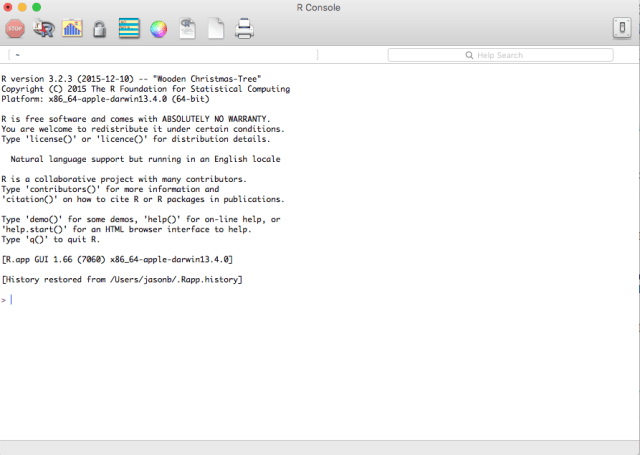
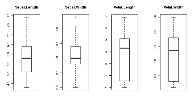
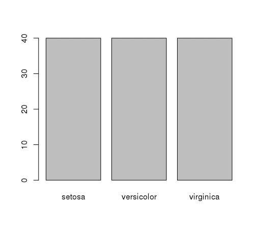
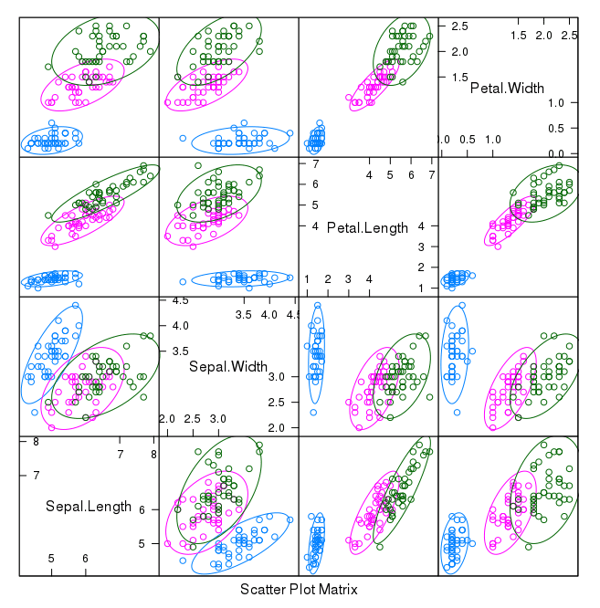
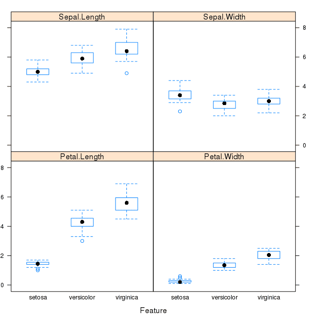
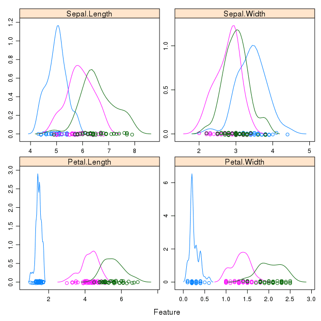
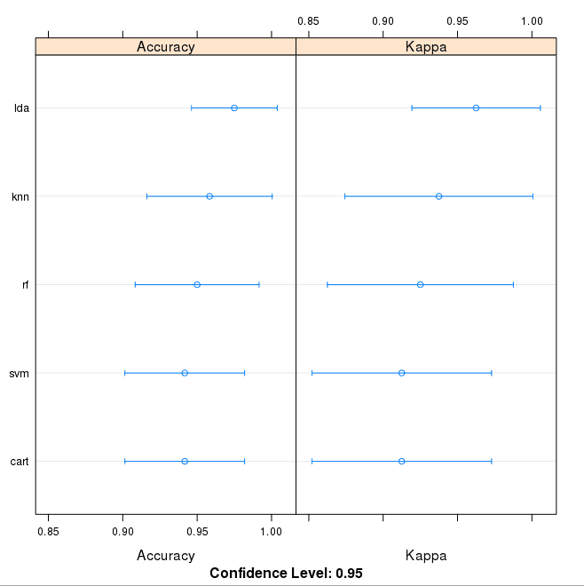


This is what I can’t stand about open-source packages like R (and Python, and LibreOffice): Nobody puts in the effort required to make sure things work properly, it’s almost impossible to duplicate working environments, and the error messages are cryptically impossible. Trying to generate the scatterplot matrix above, cutting and pasting the command into R, I got the following error message:
Error in grid.Call.graphics(L_downviewport, name$name, strict) :
Viewport ‘plot_01.panel.1.1.off.vp’ was not found
Google Search provided no help. After getting featurePlot to work with all options other than “ellipse”, finally stumbled across the solution that you needed to have the “ellipse” package installed on your system. I’m guessing that you have that as a default library on your system, so you didn’t specify it was required to use that function. But how many people reading this post will be able to figure that out?
Thanks for pointing that out Leszek. To be honest I’ve not heard of that package before. Perhaps it is installed automatically with the “caret” or “lattice” packages?
Thanks for the post… worked after installed ellipse package. not installed with caret.
Glad to hear it Rajendra.
Yet it works after installing ellipse packages
Nice!
Thanks for the post. I tried Google first when I saw the error, interestingly the 5th search result is the link back to this post. 🙂 It works after installing ellipse package.
Thanks Jason for this great learning tutorial!
Glad to hear it!
the most important piece of information missing in the text above:
install.packages(“ellipse”)
Thanks Rajendra !!!
Thanks for the tip!
He did not have the “ellipse” package as default on his system. What he did was that he installed the “caret” package using the code he provided above:
install.packages(“caret”, dependencies = c(“Depends”, “Suggests”))
The result was that ALL the packages that were likely to be used by the “caret” package were also installed… including the “ellipse” package. You could have avoided your frustration by simply following the instructions in the tutorial.
Wrong. I followed the instructions exactly as listed and it didn’t work for me either. When I explicitly installed the ellipse library it worked fine.
Perfect remarks. Always follow the instructions of the tutorial. Great tutorial Jason, as usual of course.
Thanks.
Thanks for highlighting the problem. True, it was hard to find a solution elsewhere on the Internet!
Thanks! Your comment saved me!
Hi Jason,
Recently I started with R. Great tutorials!
I would like to ask you a question, hopefully you can point me in the right direction.
Last year I bought software that develops trading systems for the stock market.
It is capable to generate thousands of trading systems in a day,
The price history can be cut in three parts: in sample, out of sample and validation.
For every trading system and every price part I have metrics like: net profit, drawdown, average trade result and so on.
I would like to use the in sample and out of sample results (metrics) to try and predict the results (metrics) in the validation period.So I can determine what trading systems perform the best accoridng to the in sample and out of sample metrics and the algorithm.
What algorithm can you advice me to use in this particular case?
Thanks again Jason!
Sharon
I don’t know about predicting stocks, as far as I have read a persistent model is the best you can do. More here:
https://machinelearningmastery.com/faq/single-faq/can-you-help-me-with-machine-learning-for-finance-or-the-stock-market
Nevertheless, I recommend this approach to evaluating time series models:
https://machinelearningmastery.com/backtest-machine-learning-models-time-series-forecasting/
I wonder how I should write to evaluate one single case.
Assume I build a model which will categorise fruits . I build a model and train it with data.
But how do I do when all this is finished and I want to test one single case?
“What fruit is this?”
Perhaps this will help:
https://machinelearningmastery.com/train-final-machine-learning-model/
Thanks for commenting! I had the same problem.
While executing, “Create a Validation Dataset” codes, I am getting the error as:
Error in createDataPartition(dataset$Species, p = 0.8, list = FALSE) :
could not find function “createDataPartition”
and same in Multivariate Plots codes,
Error in featurePlot(x = x, y = y, plot = “ellipse”) :
could not find function “featurePlot”
What shall I do?
This might help:
https://machinelearningmastery.com/faq/single-faq/why-does-the-code-in-the-tutorial-not-work-for-me
Same….did it solve?
And, moving on, found that there were additional packages that needed to be installed and loaded, and then wound up with an Accuracy table that didn’t get the same results as you did, despite copying and pasting all the commands exactly as written. This doesn’t give me a lot of confidence about reproducibility in R.
Post your results!
It is true that strictly reproducible results can be difficult in R. I find you need to sprinkle a lot of set.seed(…) calls around the place, and even then it’s difficult.
The reason why your accuracy table is not the same mainly comes from the fact that the “createDataPartition()” function chooses observations in the dataset randomly. This means that the training and validation datasets are essentially different for everybody. Consequently, the end results will be slightly different.
Yup ..
That’s a good point about createDataPartition(). I’m adding a setSeed() right before that.
Hi Jason,
When i loaded the caret package using below query,
> require(caret)
Output:
Loading required package: caret
Error in loadNamespace(j <- i[[1L]], c(lib.loc, .libPaths()), versionCheck = vI[[j]]) :
there is no package called ‘pbkrtest’
In addition: Warning message:
package ‘caret’ was built under R version 3.2.3
I have assigned the iris dataset to dataset2. then i executed the below query
createDataPartition(dataset2$Species, p=0.80, list=FALSE) is not working. I am getting the error message when i execute the above query.
Error Message:
Error: could not find function "createDataPartition"
Let me know as what went wrong.
Regards,
Mohan
This looks like a problem specific to your environment. Consider re-installing the caret package with all dependencies:
install.packages(“caret”, dependencies = c(“Depends”, “Suggests”))
I’ve added this command to the install packages section, just in case others find it useful.
Hi,
If the R version is 3.2.1 or below the caret package may turn incompatible. I faced similar issue. After uninstalling the old version I installed R 3.2.3 which fixed the error.
Hope it helps.
-Rajesh
Thanks Rajesh, I updated the post and added a note to use R 3.2.3 or higher.
Thanks for sharing this. I had to grab another package (kernlab) to run the SVM fit, but everything rolled smoothly, otherwise. Great 15min introduction!
Great to hear, thanks CW!
Hello Jason, this is an interesting tutorial and getting to grips with Caret still. Qs is: in the sctarrerplot matix(which is used from caret I think) how do we know what colours corespond to which class Rgds Ajit
That is a good question. It is a good idea to add a legend to your graphs.
I did not add a legend in this case because we were not interested in which class was which only in the general separation of the classes. Type ?featurePlot to learn more about adding a legend.
Thanks Jason. But more to the point .. where in the code do you assign the legend(or does the legend get picked up automatically ie which colour to which class. If it does so implicitly, how do I know what colour coresponds to what class?
Also another question
It says “We will 10-fold cross validation to estimate accuracy. This will split our dataset into 10 parts, train in 9 and test on 1 and release for all combinations of train-test splits. We will also repeat the process 3 times for each algorithm with different splits of the data into 10 groups, in an effort to get a more accurate estimate.” Hence I should expect to see 15 steps(3 times per algorithm with different splits) but we see here 5 steps(once) where do we try the other two times? kind rgds Ajit
Hi Ajit,
The repetitions should be indicated in the trainControl function. When I was reading, I though 3 was the default, but this didn’t seem to be the case according to the documentation ?trainControl
According to this (http://stats.stackexchange.com/questions/44343/in-caret-what-is-the-real-difference-between-cv-and-repeatedcv), the
methodparameter should have been “repeatedcv” and not just “cv”, and then the parametersrepeatsshould have been 3.trainControl(method=”repeatedcv”, number=10, repeat=3)
You can verify that the training takes longer and the confidence intervals of the plots are smaller, so I might be right. However, I am not absolutely sure if this is correct, because I don’t know how to visually check the folds. Also, I don’t know how to get each individual result of each cv and repetition from the fits, e.g. fit.lda.
Cheers
Thanks Jason for the great tutorial. I was able to reproduce the same results by following your instructions carefully. BTW, I reviewed some of the other posts above and most of the dependencies could have been resolved by loading the library(caret) at the beginning. I did encounter one issue prior to loading the library(caret) with the Error: could not find function “createDataPartition”. This error was resolved by loading the required library(caret). This loaded other required packages.
> library(caret)
Loading required package: lattice
Loading required package: ggplot2
>
Happy coding / earning!
Thanks Kiri.
If anyone wants more practice, I did my best to recall the code Chad Hines and I added to the tutorial so one can examine the mismatches for LDA on the training set. Thank you to Jason Brownlee for this tutorial and to Kevin Feasel and Jamie Dixon for coordinating the .NET Triangle “Introduction to R” dojo last week.
https://github.com/RickPack/R-Dojo/blob/master/RDojo_MachLearn.R
Correction: Chad Kimes
Thanks Rick
Hi Jason Brownlee,
Thanks for your tutorial. However, I have a question about featurePlot function with plot = “density ” option. I couldn’t figure out the meaning of vertical axis in these plots for each features. Why the vertical axes have values that are greater than 1 (in the case of density)
Hi Jason, very thorough and great practice for a newbie like myself. I will definitely be referring back to this one often.
I’m glad you found it useful Johnny.
Thanks, Brownlee. I would like to know of selecting best model. Is it guaranteed that a model giving highest accuracy can give the result of highest accuracy for test data? In this example, you have selected lda as the best model comparing the accuracies of the used models. But it may not predict best during testing. So my question is: when should we select our model? After training models or testing models?
We cannot be sure we have picked the best model.
We must gather evidence to support a given decision.
More testing with k-fold cross validation and hold-out validation datasets can increase our confidence.
So, what is next?
What can one do to get better at this? Any practice? Anything that builds on this?
What happens when there is “noise” in the data, how do we clean it and apply it to ML properly?
Great question Justin,
My advice is to practice on a suite of problems from the UCI ML Repo, then once you have confidence, start practicing on older Kaggle datasets.
Here’s a great list of datasets to try:
https://machinelearningmastery.com/tour-of-real-world-machine-learning-problems/
Tested in rstudio-ide. Works fine! Two small changes required:
-1-
# Install Packages
install.packages(‘caret’, repos=’http://cran.rstudio.com/’)
library(caret)
-2-
# e1071
install.packages(‘e1071’, dependencies=TRUE)
Nice one, thanks for sharing Jerry.
which of the algorithms require e1071? I was able to run all but had to (or R did it itself) install packages rpart and kernlab.
e1071 provides various algorithms used by caret. Learn more here:
https://cran.r-project.org/web/packages/e1071/index.html
Is this a typo on this page?
“A machine learning project may not be linear, but (it has a has) a number of well known steps:”
Yes, I intended to talk about the process of a machine learning project not being linear.
I’ve fixed the typo, thnaks.
Indeed it is good post, but as it is framed in the mind for ML Learners, would have explained in details of each section much more clear, for ex, 4.1 barplot section, would have explained understand number of diagram. mere walk-through would not help anything
Thanks for your feedback Rajendra.
Excellent, thank you, managed to do this with my own dataset but struggling to plot an ROC curve after. Please can you help by posting the code to plot the ROC curve? thanks
Sorry I do not have an example Stef, see the pROC package: https://cran.r-project.org/web/packages/pROC/index.html
Thanks Jason, will take a look.
I have just started learning R and trying to use this Tutorial to fit my Dataset into it, and had a few problems like missing packages, I did however notice that when you library(caret) it will say what is missing so it’s a simple case of install.packages(missing package displayed).
I would however like to split my dataset up a bit more, this tutorial uses
“validation_index <- createDataPartition(dataset$Species, p=0.80, list=FALSE)"
My dataset is pretty large and I would like to split it into 3 or 4, like rather than an 80/20 split I would like a 50/25/25 or a 40/30/30. As I said I'm new to R so if my way of splitting it isn't the way it should be done just tell me :).
Hi Lewis,
I believe createDataPartition() is for creating train/test splits.
You could use it to create one split, then re-split one of the halves if you like.
I hope that helps.
Very Nice article. Thank you. It was a very good starter for me as a new R programmer.
But one question I have is in section 6 (“Make Predictions”).
I understand that we are predicting the accuracy of our model in that section. But can you please elaborate on how to make prediction for some new data set ? I am not clear in that prediction part.
This is very helpful. Thanks. But I have a question. In a case where I have two datasets, will name them trainingdata.csv and testdata.csv, how do I load them to R but train my algorithm on training data and test it on the data set?
thanks.
This post will help you load your data:
https://machinelearningmastery.com/how-to-load-your-machine-learning-data-into-r/
I know how to load this data. My question is if I have two data sets, the training data and the test data. What functions must I use for R to recognise my training data to built the models on and test data to validate. Unlike on the Iris project where they have one data and splitted it on 80% 20%
Sorry, I don’t understand your question. Perhaps you can rephrase it?
on the iris project, am getting an error for the function to partition data. See below commands.
> #attach the iris dataset to the environment
> data(iris)
> #rename the dataset
> dataset # create a list of 80% of the rows in the original dataset we can use for training
> validation_index validation_index <- createDataPartition(dataset$Species, p=0.80, list=FALSE)
Error: could not find function "createDataParti
Check that you have the caret package installed.
Great post, thanks. I got it working. But when I replaced my data with iris, I got an error:
“Metric Accuracy not applicable for regression models” for all non-linier models. Here is my data:
https://www.dropbox.com/s/ppg0zdfuzz7p0mo/MyData.csv?dl=0
Any suggestions?
It sounds like your output variable is a real value (regression) and not a label (classification).
You may want to convert your problem to classification or use regression algorithm and evaluation measure.
Thanks for an excellent post Jason, great help!
You’re welcome Jonatan.
Thank you sir ! This is really the best tutorial . I learned a lot from it and i applied it to a different dataset . But how about comparing the models using ROC curve using the caret package ?
I’m glad to hear it.
Great suggestion!
In Multivariate Plots, while trying to scatterplot matrix I am getting following error:-
Error in grid.Call.graphics(C_downviewport, name$name, strict) :
Viewport ‘plot_01.panel.1.1.off.vp’ was not found
I am using R x64 3.4.0.
Sorry, I have not seen that error before. Perhaps post it as a question on stackoverflow?
This was solved. Please check in discussion.
1) You have to install ‘ellipse” package. which is missing
install.packages(“ellipse”)
2) If you change plot=pairs, you can see output. If you want, ellipse, please install ellipse package.
this is very interesting sir, but i will like help on how to better explain the plots and what each mean especially the scatterplot. i am saying in a situation where i would have to explain to an audience
You can learn more about scatterplots here:
https://en.wikipedia.org/wiki/Scatter_plot
for print(fit.lda), I don’t see Accuracy SD or Kappa SD printed/displayed … any hints? Thanks.
I think caret API has changed since I posted the example.
use fit.lda$results to show the standard deviations
good job Jason , but can I plot the SVM results in R? So I get the hyperplane and support vector points
You may, I have not done this myself in a long time. I do not recall the function name off-hand sorry.
Hello Jason! Thanks for making this ML tutorial. I am having trouble in the model building part. I am getting error in “rpart”, “knn”. When I run the code for rpart, the error is “Something is wrong: all the accuracy metric values are missing:” “Error: Stopping” “In addition: There were 26 warnings (use warnings() to see them)” , however for “knn”, the last error line I am getting 50 warnings.
Also , when I run “svmRadial” , it seems to run without any problem, however when i run the code for ‘rf”, I get this
Loading required package: randomForest
randomForest 4.6-12
Type rfNews() to see new features/changes/bug fixes.
Attaching package: ‘randomForest’
The following object is masked from ‘package:dplyr’:
combine
The following object is masked from ‘package:ggplot2’:
margin
I have a Version 1.0.136 of RStudio. Your help is much appreciated!
I’m sorry to hear that. Ensure you have the latest version of R and the caret package installed. You may also want to install all recommended dependencies.
Do you have such an R tutorial for regression problems too?
Yes, search “R Regression”
This post is exactly what I was looking for. Very well put together and I’m excited about it. I will share it with some students over at UCSF. For those reading the comments, I typed everything in manually directly from Dr. Brownlee’s scripts. You learn more that way because you’re likely to make a mistake when typing at some point.
Thanks Sunny, I’m glad you found it useful!
this post helps a lot but need little more clarification about boxplot and barchart becoz i am new for ml and r.could u plz explain me…it would be more helpful for me
what does this code tell us.cant understand plz help me
par(mfrow=c(1,4))
for(i in 1:4) {
boxplot(x[,i], main=names(iris)[i])
}
It creates a composite plot of 4 boxplots side by side.
sudi,
par(mfrow=c(1,4)) /this code specifies the gui enable a graphical display of 1 row with 4 columns
for(i in 1:4) { / this line means for each column in columns 1:4 do the follow in { code block}
boxplot(x[,i], main = names(iris)[i) / make a boxplot of the data for the column, labeled w col name
}
Thank so much sir. This is very helpful. Sir, I have a question.
When I run LDA, SVM, RF, CART model always shows that Loading required package: MASS for LDA and so on for all methods that you mention. Although I get the results without loading specific package for each methods,but is it any problem if load the specific package or not?
And if I load the package for each methods then function will be change such as for random forest we need to call the model:- randomForest(…) with package “randomForest”.
It is normal for caret to load the packages it needes to make predictions.
Hi, I have installed the “caret” package. But after this when i am loading through library(caret), I am getting the below error:
Loading required package: ggplot2
Error: package or namespace load failed for ‘ggplot2’ in loadNamespace(j <- i[[1L]], c(lib.loc, .libPaths()), versionCheck = vI[[j]]):
there is no package called ‘munsell’
Error: package ‘ggplot2’ could not be loaded
I’m sorry, I have not seen this error. Perhaps check on stackoverflow if anyone has had this fault or consider posting the error there.
Hi Jason,
Post some R&D was able to resolve it. Below are the actions i did.
install.packages(“lattice”)
install.packages(“ggplot2”)
install.packages(“munsell”)
install.packages(“ModelMetrics”)
library(lattice)
library(munsell)
library(ggplot2)
library(caret)
Nice work, glad to hear you figured it out.
Hi Jason,
Need one help again. Thanks in advance.
Since this is my first Data Science Project, so the question.
What and how to interpret from the result of BoxPlot. It will be of help if you can kindly explain a bit of the outcome of the BoxPlot.
The box plot shows the middle of the data. The box is the 25th to 75th percentile with a line showing the 50th percentile (median). It is a fast way to get an idea of the spread of the data.
More here:
https://en.wikipedia.org/wiki/Box_plot
Hello Dr Brownlee,
I am new to machine learning and attempting to go through your tutorial.
I keep getting an error saying that the accuracy matrix values are missing for this line:
results <- resamples(list(lda=fit.lda, cart=fit.cart, knn=fit.knn, svm=fit.svm, rf=fit))
The accuracy matrix for lad works however cart, knn, svn and rf do not work.
Do you have any suggestions for how to fix this?
Thanks
I’m sorry to hear that. Confirm your packages are up to date.
sir, how could i plot this confusionMatrix “confusionMatrix(predictions, validation$Species)”?
Looks good.
> predictions confusionMatrix(predictions, validation$Species)
Error in confusionMatrix(predictions, validation$Species) :
object ‘predictions’ not found
Could anyone clarify this error ?
predictions confusionMatrix(predictions, validation$Species)
Error in confusionMatrix(predictions, validation$Species) :
object ‘predictions’ not found
Could anyone clarify this error ?Earlier I posted something wrong
Perhaps double check that you have all of the code from the post?
got the same error how should i solve it?
Hi,
I am beginner in this so may be the question I am going to ask wont make sense but I would request you to please answer:
So when we say lets predict something, what exactly we are predicting here ?
In case of a machine (motor, pump etc) data(current, RPM, vibration) what is that can be predicted ?
Regards,
Saurabh
In this tutorial, given the measurements of iris flowers, we use a model to predict the species.
set.seed(7)
> fit.lda <- train(Species~., data = data, method = "lda", metric = metric, trControl = control)
The error i got, and also tried to install mass package but it not getting installed properly and showing the error again and again please help me sir.
ERROR:-
Loading required package: MASS
Error in unloadNamespace(package) :
namespace ‘MASS’ is imported by ‘lme4’, ‘pbkrtest’, ‘car’ so cannot be unloaded
Failed with error: ‘Package ‘MASS’ version 7.3.45 cannot be unloaded’
Error in unloadNamespace(package) :
namespace ‘MASS’ is imported by ‘lme4’, ‘pbkrtest’, ‘car’ so cannot be unloaded
Error in library(p, character.only = TRUE) :
Package ‘MASS’ version 7.3.45 cannot be unloaded
I’m sorry to hear that. Perhaps try installing the MASS package by itself in a new session?
Hello Jason,
My question is regarding scaling. For some algorithms like adaboost/xgboost it is recommended to scale all the data. My question is how do I unscale the final predictions. I used the scale() function in R. The unscale() function expects the center(which could be mean/median) value of the predicted values. But my predicted values are already scaled. How can I unscale them to the appropriate predicted values. I am referring to prediction on unlabeled data set.
I have searched for this in many websites but have not found any answer.
Perhaps scale the data yourself, and use the coefficients min/max or mean/stdev to invert the scaling?
I am getting an error while summarize the accuracy of models,
Error in summary(results) : object ‘results’ not found
You may have missed some code?
> library(tidyverse)
Sir while adding this library in R, I have installed the package then also it is showing following the error: please help me
Error in loadNamespace(j <- i[[1L]], c(lib.loc, .libPaths()), versionCheck = vI[[j]]) :
there is no package called ‘bindrcpp’
Error: package or namespace load failed for ‘tidyverse’
Sorry, I am not familiar with that package or the error. Perhaps try posting on stackoverflow?
Dear Jason,
I am not familiar with R tool. When I started reading this tutorial, I thought of installing R. After the installation when I typed the Rcommand, I got the following error message. Please give me the suggestion…
> install.packages(“caret”)
Installing package into ‘C:/Users/Ratna/Documents/R/win-library/3.4’
(as ‘lib’ is unspecified)
— Please select a CRAN mirror for use in this session —
trying URL ‘http://ftp.iitm.ac.in/cran/bin/windows/contrib/3.4/caret_6.0-77.zip’
Content type ‘application/zip’ length 5097236 bytes (4.9 MB)
downloaded 4.9 MB
package ‘caret’ successfully unpacked and MD5 sums checked
The downloaded binary packages are in
C:\Users\Ratna\AppData\Local\Temp\RtmpQLxeTE\downloaded_packages
>
Great work!
Hi Jasson,
I tried the following but got the error,
> library(caret)
Loading required package: lattice
Loading required package: ggplot2
Error: package or namespace load failed for ‘caret’ in loadNamespace(i, c(lib.loc, .libPaths()), versionCheck = vI[[i]]):
there is no package called ‘kernlab’
>
It looks like you might need to install the “kernlab” package.
Thanks Jasson!!!!
You’re welcome.
e1071 error i have installed all packages…..
What error did you get?
Hi All,
When I created the updated ‘dataset’ in step 2.3 with the 120 observations, the dataset for some reason created 24 N/A values leaving only 96 actual observations. Copy and pasted the code from the post above. Any idea what caused or how to fix so that the ‘dataset’ is inclusive of all the training data observations? Doesn’t seem to be anything wrong with the IRIS dataset or either of the validation_index or validation datasets.
Perhaps double check you have the most recent version of R?
Update to OP, I reran the original commands from that section and was able to pull in all 120 observations for the training data. Not sure why it didn’t fetch all the data the first time but looks ok now.
Glad to hear it.
Just confirming, the above tutorial is a multiclass problem? Therefore, I should be able to apply the above methodology to a different k=3 problem. Is this correct?
Yes.
Jason,
For my first Machine Learning Project, this was EXTREMELY helpful and I thank you for the tutorial. I had no problems going through the script and even applied to a dummy dataset and it worked great. So thank you.
My question is more related to automation. Instead of manually assessing the accuracy of each model to determine which one to use for prediction, is there a way to automatically call the model with the highest accuracy in the “predictions <- predict([best model], validation)" script. Hope to hear from you soon.
Well done!
Great question. Generally, once we find the best performing model, we can train a final model that we save/load and use to make predictions on new data. This post will show you how:
https://machinelearningmastery.com/finalize-machine-learning-models-in-r/
And this post covers the philosophy of the approach:
https://machinelearningmastery.com/train-final-machine-learning-model/
I did not get 100% Accuracy after following the tutorial example. I got :
Confusion Matrix and Statistics
Reference
Prediction Iris-setosa Iris-versicolor Iris-virginica
Iris-setosa 10 0 0
Iris-versicolor 0 8 0
Iris-virginica 0 2 10
Overall Statistics
Accuracy : 0.9333
95% CI : (0.7793, 0.9918)
No Information Rate : 0.3333
P-Value [Acc > NIR] : 8.747e-12
Kappa : 0.9
Mcnemar’s Test P-Value : NA
Statistics by Class:
Class: Iris-setosa Class: Iris-versicolor Class: Iris-virginica
Sensitivity 1.0000 0.8000 1.0000
Specificity 1.0000 1.0000 0.9000
Pos Pred Value 1.0000 1.0000 0.8333
Neg Pred Value 1.0000 0.9091 1.0000
Prevalence 0.3333 0.3333 0.3333
Detection Rate 0.3333 0.2667 0.3333
Detection Prevalence 0.3333 0.2667 0.4000
Balanced Accuracy 1.0000 0.9000 0.9500
>
Perhaps try running the example multiple times?
sir, i want to learn r programing at vedio based tutorial which is the best tutorial to learn r programming quickly
Sorry, I don’t have good advice on how to learn R, I focus on teaching how to learn machine learning for R.
For learning R I strongly recommend the Coursera.org “R Programming” certification course, When I took it it was free, now is paid, something around USD 50.
Thanks for the tip.
Json, nice article. I left working code with minor fixes in this repo, please comment on, thanks, Carlos
https://github.com/bandaidrmdy/caret-template
Thanks for sharing.
what if the dataset is used EuStockMarkets, I error continue
Sorry, I don’t know about that dataset.
successfully done, and got the result.Thanks for the great tutorial.
But now i wonder, what to do further, how to use it in a generic manner for any dataset.
How to use the created pred.model anywhere.
Yes, you can use this process on other datasets.
ohk, but to use any dataset we need to make the dataset similar to that of the iris dataset, like 4 numberic columns, and one class.
Also, accuracy output is similar over the traning dataset , and the validation dataset, but how does that help me to predict now what type of flower would be next if i provide it the similar parameters.
Now, for example i have to create a model which predicts the cpu utilization of the servers in my Vcenter or complete DC, how can i create a model which will take my continious dataset and predict that when the CPU utilization will go high and i can take proactive measures.
This process will help you work through your predictive modeling problem systematically:
https://machinelearningmastery.com/start-here/#process
Hello Jason,
Thanks for the clear and set by step instructions. But I just want to understand what I need to do after creating the model and calculating its accuracy ? Can you please explain to draw some conclusions/predictions on the iris data set we used ?
You can finalize and start using it.
See the whole process here:
https://machinelearningmastery.com/start-here/#process
Hi Sir,
For the confusionMatrix(predictions, validation$Species) command , I am getting an output as follows:
[,1] [,2]
[1,] 0 0
[2,] 0 10
I am not getting the same output as you got. Any suggestions on what I may be doing wrong.?The code worked exactly till this command.
Perhaps double check that you copied all of the code exactly?
And that your Python environment and libraries are up to date?
Hello good day Jason.
Thank you very much for the tutorial I have been very useful but I have a question, in the section of “print (fit.lda)” does not deploy “Accuracy SD Kappa SD”.
What remains of the tutorial if you have given me exact, could you help me with this doubt ?.
Greetings.
The API may have changed slightly since I wrote the post nearly 2 years ago.
Great article for a beginner like me Jason! Appreciate your work in sharing your knowledge and educating.
Is there a model fit for ‘multinomial logistic regression’ algorithm?
Thank you!
There is, but I would not recommend it. Try LDA instead.
Upon further reading of other articles written by you, I realize that I may not need to use ‘Regression’. My dataset has category variables as input and category attributes as output as well (having 7 levels). So, it is a classification problem and I’m assuming I can use one of the 5 models/fit you have given as examples here in this Iris project. Can you let me know if this is correct understanding?
– Thank you
This post may help clear you the difference between classification and regression:
https://machinelearningmastery.com/classification-versus-regression-in-machine-learning/
It works for me with the iris data. Thanks a lot Jason! But there are no “Accuracy SD Kappa SD ” from the output of the fit models. Should I change some settings to get them?
I believe the API may have changed.
Dear Jason Brownlee
I have a dataset with 36 predictors and one for classes (“1”, “2”, “3”) that I got it through clustering in the previous step.
My question is: how can I reduce all my predictors into five variables representing specific dimensions in my study?
Should I run PCA separately to produce a new dataset with 5 predictors and one for classes or is there any other ways?
Thank you in advance.
Yes, you would run dimensionality reduction first to create a new input dataset with the same number of rows.
Hi Jason, I am getting the error –
Error: could not find function “trainControl”
on typing tc<-trainControl(method="cv",number=10).
What can be the solution for this?
Perhaps caret is not installed or caret is not loaded?
Maybe a very stupid question. But I read “Build 5 different models to predict species from flower measurements”. So now I am wondering what the predictions of the model tell me about this, how I can use it. For example I now go to the forest take some measurements, assume that the flower is one of those tested, and want to know which flower it is exactly. In a traditional regression formula it is straightforward as you can put in your measurements in the formula and the calculated estimates and get an outcome. But I don’t know how to use the outcomes in this case.
Great question.
Once we choose a model and config, we develop a final model trained on all data and save it. I write about this here:
https://machinelearningmastery.com/train-final-machine-learning-model/
You can then load the model feed in an input (e.g. a set of measures) and use it to make predictions for those measures.
Does that help?
Your Tutorial is just awesome . Thanks its really helpful
Thanks, I’m glad to hear that.
This tutorial really helpful. Thanks Jason.
Thanks, I’m glad to hear that.
Hi Json how are ?
I am new in machine learning. i want to invent a unique idea and prof about islami banking and conventional banking. how can i do that. if any suggestion please give me and i cant fund any islami banking data set like loan info or deposit bla bla bla. i want your valuable information
Sorry, I don’t know about banking.
Dear Sir, I am getting the following error
Error in
[.data.frame(out, , c(x$perfNames, “Resample”)) :undefined columns selected
when i execute
results <- resamples(list(lda=fit.lda,nb=fit.nb, cart=fit.cart, knn=fit.knn, svm=fit.svm, rf=fit.rf))
What can be the solution for this?
Did you copy all of the code from the tutorial?
Hi Jason, First of all great work. May God bless you for all your sincere efforts in sharing the knowledge. You are making a big difference to the lives of people. Thank you for that.
I have a basic question. Now we have a best fit model – how to use it in day to day usage – is there a way I can measure the dimensions of a flower and “apply” them in some kind of equation which will give the predicted flower name? How to use the results? Kindly advise when you are free.
Hi Jason – found another of your post:
https://machinelearningmastery.com/deploy-machine-learning-model-to-production/
Thank you.
Hi Jason – the post was good in telling what to do. However the how part is still missing. Hence still need help. Thank you.
You can make predictions as follows:
yhat = predict(Xnew)
Where Xnew are new measurements of flowers.
Thanks.
Also see this post:
https://machinelearningmastery.com/train-final-machine-learning-model/
Dear Jason,
Thank you very much for your response. Yes – I was about to post that this link was indeed helpful in operationalizing the results.
Thank you very much. Please keep up the great work.
Hussain.
Glad to hear it.
Hi Jason,
Thank you for sharing your methods and codes. It was very useful and easy to follow. Could you please share how to score a new dataset using one of the models? For example, in my training, random forest has the best accuracy. Now I want to apply that model on a new dataset that doesn’t have the outcome variables, and make prediction.
Thank you
Great question, I answer it in this post:
https://machinelearningmastery.com/train-final-machine-learning-model/
Thanks Jason. I read through the link. I already finalized my model, now I need save the model and apply it for operational use. The dataset that I want to score doesn’t have the outcome variable. I am not sure which command I should use to make prediction after I have the final model. Can you suggest R codes to do so?
You can use the predict() function to make a prediction with your finalized model.
Hi Jason! Amazing post! I have the same doubt @TNguyen did. I Finalized the model and we know that LDA is the best model to apply in this case. How I predict the outcome variables (species) in a new dataframe without this variable? IN summary, how I deploy the model on a new dataset? Sorry, I´m new in this field and I´m learning new things all the time!
Good question, I have an answer here that might help:
https://machinelearningmastery.com/faq/single-faq/how-do-i-make-predictions
Here is a tutorial for finalizing a model in R:
https://machinelearningmastery.com/finalize-machine-learning-models-in-r/
Hey,
Thanks for the great tutorial. I have a problem and don’t know what’s wrong in the section
3.1 Dimensions. When I execute dim(datset) I get the answer NULL.
Do you know why R Studio doesn’t show me the dimensions of the “dataset”?
Best regards
Martin
Perhaps confirm that you loaded the data?
Very nice, Its given overall structure to write the ML in R.
Thanks!
Hey, I am working on the package called polisci and I am asked to build a multiple linear regression modal. My dependent variable is human development index and my independent variable is economic freedom. Could ou please tell me how can I perform multiple linear regression modal. How do I go about in steps and what is the syntax in R to get to the results and get a graph? Any help would be greatly appreciated. Please help me as I am an undergrad student and I am learning this for the first time
Thanks in advance
Sorry, I don’t have examples of time series forecasting in R.
Here are some resources that you can use:
https://machinelearningmastery.com/books-on-time-series-forecasting-with-r/
Thanks Jason,
Was able to execute the program in one go.. Excellent description
Well done!
Jason, Thank you very much for you above work. Its Ohsomesss, I am new to data science and want to make my carrier. I found so useful this superb……
You’re welcome, I’m glad it helped.
Please suggest me a path to become data scientist step by step, and how to become champion in R and python ??
Sure, start right here:
https://machinelearningmastery.com/start-here/
Thanks, Jason! This is a very helpful post. I did exactly as suggested, but when i print(fir.lda), I do not have the accuracy SD or kappa SD. How should I get them? Thanks
Perhaps the API has changed.
Amazing tutorial!
I just need to install 2 packages: e1071 and Ellipse
After that, i wrote every single line, and i really appreciate the big effoct you done to explain so clear!!!
Thank you
I’m glad it helped.
Thanks for the great tutorial. I have a problem and don’t know what’s wrong in the section
6. Make predictions . When I execute predictions <- predict(fit.lda, validation)
confusionMatrix(predictions, validation$Species) I get the error "error data and reference should be factors with the same levels."like this
Do you know why R Studio doesn’t show me the Make predictions of the “dataset”?
Perhaps try running the script from the command line?
https://stackoverflow.com/questions/19871043/r-package-caret-confusionmatrix-with-missing-categories
Please check above link ^
When I try to do the featurePlots I get NULL. I installed the ellipse package without error.
featurePlot(x=x, y=y, plot=”ellipse”)
NULL
> # box and whisker plots for each attribute
> featurePlot(x=x, y=y, plot=”box”)
NULL
> # density plots for each attribute by class value
> scales featurePlot(x=x, y=y, plot=”density”, scales=scales)
NULL
everything up to this point worked fine
I’m sorry to hear that. Perhaps there is another package that you must install?
Dear Dr Jason,
Two situations – (i) the NULL problem – rectified, and (ii) displaying multivariate graphs. and (iii) typo error
(i) The NULL problem rectified.
I too was getting the problem at section 4.2 on multivariate plots. The problem was fixed.
You were correct that another package you must install. That was in 2018. Referring to the 2019 Updated subheading at the top of the page, it is necessary to install other packages by typing:
The package on my internet connection took nearly 2 hours. But it was worth it.
(ii) Displaying the barplot in section 4.1 and multivariate graphs.in section 4.2
In order to get the barplot and multivariate plots in sections 4.1 and 4.2 respectively to display in the whole window, I would add this line:
Otherwise you will get the barplots and the featurePlots all squeezed in because the command
continued from section 4.1 and operated on barplots and featurePlots.
So as soon as you deal with barplots in section 4.1 put in this line
Also there is a typo error in section 4.2. Where it says
“Like he boxplots, we can see the difference in distribution of each attribute by class value. We can also see the Gaussian-like distribution (bell curve) of each attribute.”
Replace “Like he boxplots….” with “Like the boxplots….”
Thank you,
Anthony of Sydney
Thanks, fixed.
I was also getting same error.
You would like to check below link for the solution:
https://stackoverflow.com/questions/19871043/r-package-caret-confusionmatrix-with-missing-categories
Thanks for sharing.
Great tutorial Jason! Inspired me to look up and a learn a bit more about LDA and KNN etc. which is a bonus! Great self-learning experience. I have experience with analytics but am a relative R newbie but I could understand and follow with some googling about the underlying methods and R functions.. so, thanks!
One thing… the final results comparison in Section 5.3 are different in my case and are different each time I run through it. Reason is likely that in Step 2.3 there is no set.seed() prior. So, when you create the validation dataset which is internally a random sample in createDataPartition().. results are different in the end?
Thanks.
Well done.
Thanks. Yes, some minor differences should be expected.
Jason Brownlee you the real MVP!
hanks, I’m glad the tutorial helped.
Hello this is very helpful, but i don’t get how i should read the Scatterplot Matrix
Each plot compares one variable to another. It can help you get an idea of any obvious relationships between variables.
I have problem in this….
# create a list of 80% of the rows in the original dataset we can use for training
validation_index <- createDataPartition(dataset$Species, p=0.80, list=FALSE)
# select 20% of the data for validation
validation <- dataset[-validation_index,]
# use the remaining 80% of data to training and testing the models
dataset <- dataset[validation_index,]
1
2
3
4
5
6
# create a list of 80% of the rows in the original dataset we can use for training
validation_index <- createDataPartition(dataset$Species, p=0.80, list=FALSE)
# select 20% of the data for validation
validation <- dataset[-validation_index,]
# use the remaining 80% of data to training and testing the models
dataset <- dataset[validation_index,]
Please help me out
What is the problem exactly?
it can’t findout the objects….and function also..! what can i do?
What objects?
Jason, you’re indeed a MVP! Ran this in R 3.5.
1. install.packages(“caret”, dependencies = c(“Depends”, “Suggests”)) ran for almost an hour. May be connectivity to mirrors.
2. install.packages(“randomForest”) & library(“randomForest”) needed
Would definitely recommend this to all ML aspirants as a “hello world!”
Hearty Thanks!
Well done!
Thanks for the tips.
First I’d like to say THANK YOU for making this available! It has given me the courage to pursue other ML endeavors.
The only issue I have is that when summarizing the results of the LDA model using the print(fit.lda), my results do not show standard deviation. Do you know if this is due to a setting in R that needs to be changed?
Any help is appreciated!
Best,
Giovanni
Yes, I believe the API changed since I wrote the tutorial.
Hi!
First of all great tutorial, I followed and achieved the expected results
Really helped me overcome ML jitters. Very very grateful to you.
But I really wanted to know the mathematical side of these algorithms, what do these do and how?
Also,
it would be wonderful if you could explain things like “relaxation=free” (What does this mean?) That do not have a straight answer on Google
Thanks
Regards
Thanks for the feedback Shane.
We focus on the applied side of ML here. For the math, I recommend an academic textbook.
Very nice tutorial. The caret package is a great invent. where can I find a rapid theory of the methods to understand it better?
Right here:
https://machinelearningmastery.com/start-here/#algorithms
Thanks, Brownlee.
You’re welcome.
Jason by any chance could you:
1. Post an unsupervised Random Forest tutorial. I think Caret only supports supervised. If not could you please point me to an example other than Breiman’s
2. More specifically I am looking for a predict program that takes a saved model eg Random Forest and loops through an input .csv file with class/Type predictions. Think I have the probability figured out
Thanks for the suggestion. I generally don’t have material on unsupervised methods and I have not heard of an unsupervised random forest!
Hi Jason,
Thank you for the tutorial. This helps me greatly in my study. i am running the code for this sample contributed by Rick Pack, from https://github.com/RickPack/R-Dojo/blob/master/RDojo_MachLearn.R
When I insert my mysql database data in the dataset and try to run the above sample, I get the error:
> validation_index <- createDataPartition(dataset$containsreason, p=0.80, list=FALSE)
Error in cut.default(y, unique(quantile(y, probs = seq(0, 1, length = groups))), :
invalid number of intervals
I tried searching but could not find any instance of this error.
Please
If you have a problem with someone else’s code, perhaps talk to the about it?
Hi,
I just figured it out. The data was too sparse as I was including some unwanted columns in the dataset. Once removed, it worked fine.
Happy to hear that.
It was really amazing.. Please guide me to another projects for practice and to improve my skill set .
Thank You
Thanks. More project ideas here:
https://machinelearningmastery.com/faq/single-faq/what-machine-learning-project-should-i-work-on
this really was life saving for as it was just when i was wondering to make a structure of my exam report in climate studies. Thank You sooooooooo much
You’re welcome, I’m happy that it helped!
Working perfectly.Had to install many packages though.But all worked out well with some mouse clicks and with some Google. MY FIRST SUCCESSFUL MACHINE LEARNING TUTORIAL EVER!!!!! MANY THANKS JASON!!-Love and respects from India.
Well done!
Dear Brownlee , first of all thanks for this wonderful tutorial.
I would like to learn that when we found the most accurate model , how can we ask to our model to test further samples , ie how can we run our test for one more sample data ?
for example in your test lda was the most accurate, so if you want to ask your program to check for another data what is the code for it?
thanks
isa
You must create a final model trained on all data. Learn more here:
https://machinelearningmastery.com/train-final-machine-learning-model/
Hey Jason, I have the same question as isa, and I’ve read your post on creating a final model. How does the idea of choosing a final model and giving it unseen data to analyze translate to R code? In the code above, for instance, lets say I wanted to give one row of iris flower qualities to fit.lda and have it guess what species it was. How would I do that? Thanks for the help.
Here’s an example:
https://machinelearningmastery.com/finalize-machine-learning-models-in-r/
Hi,
Thanks for the tutorial! I copy the code and it works fin till Predictions part. I get an error: Error in eval(predvars, data, env) : object ‘Sepal.Length’ not found. Could you please help me out? Thanks in advance!
How can I analyze Gujarati language texts for readability research by using R package e1071?
I don’t know, sorry.
Hi Jason
Could you plz guide how can we get the predicted value (especially in regression) for each instance of the dataset. For instance, we have 5 variables, then how can we get the five predicted (numeric) values so that we compare these values with the actual values of the dataset.
Hi jason
I am an enthusiast of R language. I am a asst prof and research scholar so i am working on ML and R. The post was very useful. I already worked with different packages but this is very simple than all other. I need one small advice, how can i make R as favorite language for my b.tech students. They are strongly supporting python but i want to make same interest with R also.
Perhaps show things that R can do that Python cannot?
Hi Jason, I’m at my wits end here. pulled all of my hair. have given up on google. searched high and low and cannot understand/get the answer to this question.
i created a model ham/spam classifier…it’s fine. but now i want to use it on a BRAND NEW data. or run 1000 rows of brand new data through it. How the heck do i do this?
i used the predict function, it works fine on the test data but on the new data (after i’ve done all the preprocessing) i get an error of object not found … object is a word and i’m assuming it doesn’t exist in one of the sets…i haven’t a clue.
so i guess i’m missing a step somewhere? please help
Sorry to hear that.
Perhaps post your code and error to stackoverflow or crossvalidated?
Great post! Very useful. All the steps worked fine with some basic knowledge. Dependencies need to be installed.
Well done!
thank you so much, helped a lot
I’m happy to hear that.
Hey Jason Thank u so much for this usefull post. Im’doing my postdegree project about optimize a supply chain system with AI. So I would like to ask you if the best Branch to forecast demand and optimize a process like this (Supply chain) is ML with neuronal networks. where can I find more information about your courses. Thanks again Merry Christmas
Perhaps a good place to start would be here Silvio:
https://machinelearningmastery.com/start-here/#deep_learning_time_series
Hi Jason,
this was my first R experience and your tutorial helped me a lot.
Although, the was seems to be long.
For example: does “fit” support also other algorithms like e.g. tensor flow?
When I go into the help system I cannot find anything about the possible algorithms.
Best,
Fred
Well done!
In this tutorial we did not use the algorithms directly, instead we used a helpful wrapper called: caret.
You can learn about using the algorithms directly, but you must refer to and learn how to use each individual R package, which may be time consuming.
hi jason,
can i use this for real time data analysis.please reply
Perhaps.
hi Jason,
nice tutorial. All worked fine for me except when trying to fit the linear algorithm “lda”.
No matter which variables I’m using (I also tried with your example).
I get this error:
Something is wrong; all the Accuracy metric values are missing:
Accuracy Kappa
Min. : NA Min. : NA
1st Qu.: NA 1st Qu.: NA
Median : NA Median : NA
Mean :NaN Mean :NaN
3rd Qu.: NA 3rd Qu.: NA
Max. : NA Max. : NA
NA’s :1 NA’s :1
Error: Stopping
In addition: There were 11 warnings (use warnings() to see them)
The rest of models work perfectly.
Thanks in advance,
J
Perhaps the API has changed since the post was written, maybe skip that algorithm?
Thank you Jason this tutorial is awesome,.and man you got amazing patience
Thanks.
Very nice tutorial!!
I was wondering: after I get a good model that can make good prediction on new datasets, how can I say which parameters are more important for the prediction? In other words, which are the important features? For example In this case I can say that I.Setosa has short sepals and short petals (etc…). But can I get the same information printed from the script?
Thanks in advance!
Perhaps try an ablative experiment, where you refit the model with each feature removed in turn, and see which feature or features negatively impacts the performance of the model the most?
Thanks Jason. I have a concern about dividing my dataset into 3: 70% for training, 15% for validation and 15% for testing.
How do I divide this. Would I have to use the caret package?
inTrain <- createDataPartition(y = data$CSC, p = 0.70, list = FALSE)
or do I have to make the validation as part of the training.
I don't understand how to divide for validation before testing and why it's necessary…
I need a detailed description to this and the R code for it if possible. I couldn't find something concise relating to this online.
Please help
Perhaps split into train/test first then split train into train/validation?
More on why validation is required here:
https://machinelearningmastery.com/difference-test-validation-datasets/
Hi,
It was a good tutorial for me.
But I’m getting this,
Error in createDataPartition(fhg$
Historic_Glucose(mg/dL), p = 0.8, list = FALSE) :could not find function “createDataPartition”
How do I get this working?
Ensure that caret is installed and loaded.
It was installed and loaded. I referred other sources and I loaded other supporting packages to get it running.
Thanks
Well done!
what packages did you load for this
Hello jason, thank you for this demo on this algorithms. The explanation was quite clear and to the point.
However, my question is, i use the above code to run a project but in the models i got some errors here is the descrription of my data..
1. i have 19 predictors and 1 response variable. but the response is categorical 1 for yes and 0 for no.. so i import the data and step by step follow your code but in the models, i use “metric = metric” but that does not work so i use “metric = Accuracy” in that as well, i got an error in using LDA, kNN and almost all the models and the error says this cannot be run on regression. but my outcome is categorical and initially i change it into factor. after all error,
2. the second part was, i now use data with 19 predictors and i use an outcome variable of 3 levels instead of 2. but this time i just maintain “metric = Accuracy” and this runs on all models without any error. the the only error results in the portion where i want to do the prediction..below is the error that result when i want to do the prediction
“Error:
dataandreferenceshould be factors with the same levels.” what does this error means?thank you and i need your response in both of my questions.
Perhaps you need to convert the output variable in your data from numeric to a factor? try as.factor() for the variable.
Hello Jason;
Thank you very much for the informative tutorial. I may miss some point here, each time I run the algorithm, I got different results. I mean that at one-time LDA was the most accurate model, another time kNN was and another time LDA, Cart, and rf had the same accuracy value. Surely, each time another train data set was used but the results were confusing. One thing, how can I see the coefficients of the models or can I?
Thank you in advance
You can expect small differences over time given changes to the how the algorithms may have been implemented/updated.
Also, differences in the random seed, more details here:
https://machinelearningmastery.com/randomness-in-machine-learning/
hello Jason’
Thank you, your tutorial is very useful for my work. May I ask one question, how can add lebels of each line in the plot (blue pink and green line) as their species (“setosa” “versicolor” “virginica”) in “Density Plots of Iris Data By Class Value” ?
Thank you very much
Hello Jason,
Very good tutorial.
I am getting an error-
> set.seed(7)
> fit.lda <- train(Species~., dataset=dataset, method="lda", metric=metric, trControl=control)
Error in terms.formula(formula, data = data) :
'.' in formula and no 'data' argument
Please suggest – how to fix the error ?
Sorry to hear that, I have some suggestions here:
https://machinelearningmastery.com/faq/single-faq/why-does-the-code-in-the-tutorial-not-work-for-me
Hi! Like others, I’m having trouble with the featureplot line. I tried updating R, and installing “ellipse” by itself and finally used the additional code for installing caret with the additional specifications. I am still getting “error in featurePlot (x=x, y=y, plot= “ellipse”) : could not find function “featurePlot”.
Any help would be appreciated.
Ignore/delete above pls, the packages were not properly installed and it’s all good now 🙂
Glad to hear you worked it out!
Thank you very much Jason! You are a great tutor. Extremely helpful. I did not manage to install the caret package in R (got some error message which I couldn’t solve) but your tutorial worked perfectly for me in RStudio.
Glad to hear it.
I am italian student, i want find from these 4 classifier method ( Multinomial regression, Discriminant analysis (linear or quadratic), KNN
classifier ) the best in terms of minimum number of misclassified records and why ? with comment and consideration. The input is IRIS dataset end the goal is perform the classification of the data in terms of the attribute in
column 5, labeled “species” (with values: setosa, versicolor, and virginica),
with respect to the four measurements: “Sepal.length”, “Sepal.width”,
“Petal.length”, and “Petal.width”, presented in columns 1-4
please help me! i want learn
Perhaps try working through the above tutorial first?
Hi Jason,
Awesome post for R beginners like myself.
I have some questions:
1) My dataset is quite higher compared to Iris’. I have 170 columns (different variables) and 4000 rows, but around 3-8% data is missing in each column. I have found that we could either impute these missing data point with the median, mean or not include them in the analyses. I am going for the median, but is this better than no analysing them?
2) For learning purposes, I have chosen 13 columns (those virtually with no missing data) + all rows and it works fine with values around or bigger than 98%. However, when using all columns the accuracy/sensitivity, etc drops to around 60%. So, is this “Ok” if I include those variables that influence the most?
3) When a database has missing data, the box and whisker plot doesn’t come up (4.1. Univariate plots). I usually get “error in call.Graphics….” or columns not define.
Hope you can clarify this questions,
Thank you for your help.
Best regards,
Alan
Perhaps try different methods for handling missing data to see what results in the best model skill.
Sounds good, continue using results to guide decisions with the modeling.
Perhaps the missing data needs to be marked as na, or perhaps the plot function needs to be told to ignore na?
Hi Jason. This step by step guide is so useful for as a beginner in machine learning.
i try to slightly modify the codes to fit my own data run the algos to model a credit risk based on logistic regression output.
Perhaps you want to share how can i modify your codes to model a credit risk model?
Thanks for the suggestion.
Thank you for posting this fantastic tutorial. I am very new to machine learning and have a quick, and probably naive, question.
How can I see the final equation which is used to predict a classification? The iris dataset and another dataset of my own convinced me how effective this can be. I would like to know the weight of each variable in determining the predicted classification.
Most models don’t give an equation, they are too complex, or if they can, it would not be readable.
Hi Jason, thank you for this post! It is very helpful. I wonder if the equation cannot be seen, are there any other ways for us to see which variables are the most influential ones in the model for predicting an outcome?
Hello sir I am new to R thanks for your above first project explanation,
now my doubts,
1. my file is excel contain more than 1000 rows with nearly 20 columns (with names) last column class ( 2 classes like yes no) in other columns some collumns values are numbers and some 4 columns having string (one column values like Yes, No and another column values like 11 Place names etc.) to do above give your first R project can I apply (excel convert as) csv file or I apply after convert string column values to numeric, if yes is can I give 1,2,3,4,5,6… different places names respectively.
2. How I use these R to do my research for my above said dataset for classification or to analysis by change some thing in classification methods.
Thank you,
By
Suresh Kumar
Yes, you can load your file as a CSV and you might want to take some time to convert the categorical fields to factors in R.
A good place to get started with R for machine learning is here:
https://machinelearningmastery.com/start-here/#r
Hi Sir!
Can You help me out, I’m working with my Final Year Project and accidentally we choose the Artificial Intelligence Project. In our project, we need to implement Artificial Neural network. It is base on student academic performance predictions, where we will predict which fields are best for the student in future studies by using their past academic data. Now even I don’t know where to get start.. remaining module of our app has been done but we are stuck in this last module. Can you help me how we should start which tools are used for code and how we will train our network depending upon student classifications? after getting training, we have to integrate it with our android studio project. Please Help!
Thanks in advance!
I’m zero in machine learning.. so please give me some time for ur kind reply.. guide me where i should start which tools should i used for it..
Start here:
https://machinelearningmastery.com/tutorial-first-neural-network-python-keras/
And then here:
https://machinelearningmastery.com/start-here/#deeplearning
Hi Jason,
How can I plot ROC on caret?
Sorry, I don’t have an example.
Jason,
Thanks for the great post. I’m a beginner in this and have a couple of perhaps dumb questions:
1. For each of the 5 models, especially the random forest one, how do I find out the chosen parameters of the models? For example, for rf, which predictors are used? what are the parameters for each of the predictors to predict the results?
2. how do I know what the predictions will be for a new set of data? In other words, if we provide a new set of values for “Sepal.Length”,”Sepal.Width”,”Petal.Length”,”Petal.Width” and want to know what the model predicts the species is, how do I do that?
Thanks.
Yue
We don’t so much care why a model works, only that it works. This is called model interpretability:
https://machinelearningmastery.com/faq/single-faq/how-do-i-interpret-the-predictions-from-my-model
We can make a prediction on a new data using a fit model, e.g. by calling predict()
hi jason Brownlee..great work published by you thanx….while running the code i am facing these errors….i have copied the code plus errors here.kindly guide me whats the problem?
set.seed(7)
> fit.knn # c) advanced algorithms
> # SVM
> set.seed(7)
> fit.svm # Random Forest
> set.seed(7)
> fit.lda fit.rf <- train(Species~., data=dataset, method="rf", metric=metric)
Error in metric %in% c("RMSE", "Rsquared") : object 'metric' not found
You may have missed a line where metric was defined.
i want c0de for one class classification gaussian algorithm
Perhaps start with a google search?
Hi Jason,
library(e1071)
set.seed(7)
fit.svm <- train(LoE_DI~., data=dataset2, method="svmRadial", metric=metric, trControl=control)
print(fit.svm)
It is taking more time to run?
like more than 1.5 hours?
is there any package i need to install to make it run faster?
Perhaps try less data?
Perhaps try an alternate model?
Great Tutorial
Thanks
You’re welcome.
This was very helpful. Thanks Jason.
Thanks, happy to hear that.
Hi Jason,
Thanks for such a wonderful guide. Can you please explain how to interpret the scatterplot matrix? I can understand if we use it to plot the relationship between two variables. I am not able to understand the relation between 3 variables through the graph that you have plotted in this tutorial.
Yes, each cell of the matrix shows one variable vs another, all cells show all variables against all other variables.
It can help to see any obvious inter-variable dependencies.
Do you know of a working example of the Dodger Loop Sensor problem? I am currently stuck trying to merge the two data csv’s and use the correct columns.
What is Dodger Loop Sensor problem?
https://archive.ics.uci.edu/ml/datasets/dodgers+loop+sensor
Using the dat from the two data file build a predictive model to predict the occurrence of a baseball game based on the loop sensor data. I am stuck trying how to clean and combine the data. It seems no one has ever tackled this problem… I am stumped. Any help would be appreciated.
Thanks for sharing.
Thanks for the great tutorial. Can you tell me how to display the confusion matrix for the cross-validation step (sums and/or mean)? While evaluating the 20% validation subdataset is informative, I have a very small dataset so it would be more informative if I could see the confusion matrix from the cross-validation step.
Generally confusion matrix is used for a single train/test split, not a k-fold cross validation.
Thank you Jason, this website and it’s tutorials are fantastic! I’ve read a lot of textbooks and currently working in the field, but still feeling a bit confused until I came across your site. You make it so easy! Thank you so much.
Thanks Kim, I’m happy to hear that!
I am very much new to machine learning, what exactly did this predict at last?
We predicted flower species from measurements of flowers.
Hi! Thanks for providing this tutorial. I am working on a project that is very similar to your example–the difference is that it is linear regression. I’m using the caret package and the train function with “full model”, “forward selection/leapForward”, and “ridge regression” and using the metric “RMSE” as the performance metric. I need to select the model with the lowest “RMSE”. I am using pretty much thes same script you are in the example. My problem is that I’m lost in the theory of what I’m doing. Here’s what I know and where I get lost:
1) created train set and test set
2) pre-processed the train set — centered, scaled, and removed non-zero variance features
3) set up the train control
4) built the 3 models
5) compared the results using “resamples”
6) picked the model with the lowest RSME (which was the forward_selection/leapForward model)
7) Used “predict” to compare the observed values to the predicted values of the forward selection
8) Finally, I created a table that shows the errors between the observed and predicted results and plotted those.
What do I do next? When using “lm”, you get a summary statistic that shows the coefficients, p value, r-squared — but how do you do this with “leapForward”?
I used “VarImp” and found that with the forward_selection model, there is only 1 feature that is highly correlated — do I then use this to run another linear regression using that 1 feature?
I’m close to understanding but not close enough to figure out what to do next…
Would very much appreciate a response to this as well, for I’m stuck on the “next” step after building the model. Can we predict completely NEW data points using this newly built model and not just use it as a comparison to train vs test data?
Appreciate all of your work!
This might help
https://machinelearningmastery.com/finalize-machine-learning-models-in-r/
Sir, my name is surya, iam from indonesia, i want to ask you, may i translate your machine learning ebook for teaching and commercial needs?
No, please do not. I explain more here:
https://machinelearningmastery.com/faq/single-faq/can-i-translate-your-posts-books-into-another-language
I have the same issue as Muriel. I did not get the caret package installed when i invoked
“install.packages(“caret”, dependencies=c(“Depends”, “Suggests”))”. Can i independently download the caret package from anywhere and install it in R?
Sorry to hear that.
No, you must install it using install.packages()
Jason, this is a very well made tutorial. It is really helpful for me – yes, there might be some issues with additional packages, like e1071, which has to be installed on the fly in my case.
But as longer one sits with this one, the better he understands. Just have to get my hands on more projects like that.
I come from Power BI side of things, want to delve deeper into data analysis and.. yes, machine learning and AI – who knows!
Great tutorial, really appreciated.
Thanks Raivo.
Dear Jason,
Many thanks for your help. I have a question. After I tested the best model on the test dataset, how can I apply the model on new unlabeled data (e.g. to classify patients or healthy individuals) or to classify even a single individual (ill vs. healthy) based on data of the model?
Is there a code for this?
Many thanks
You can call predict()
See this tutorial:
https://machinelearningmastery.com/finalize-machine-learning-models-in-r/
For step 4.2, I get the following message:
Error in stack.data.frame(x) : no vector columns were selected
Sorry to hear that, perhaps this will help:
https://machinelearningmastery.com/faq/single-faq/why-does-the-code-in-the-tutorial-not-work-for-me
#since the input ariables are numneric we create box and whisker plots
> par(mfrow=c(1,4))
> for(i in 1:4) {
+ boxplot(x[,i], main=names(iris_train)[i])
+ }
Error in oldClass(stats) <- cl :
adding class "factor" to an invalid object
getting an error here please help
This may help:
https://machinelearningmastery.com/faq/single-faq/why-does-the-code-in-the-tutorial-not-work-for-me
I really needed this Hello, World type of ML project. Thank you!
I studied the whole book Data Science in Business, which is great for a conceptual understanding. Their intention is explicitly not to cover algorithms. Still, a whole semester of nothing concrete failed to build my confidence.
I don’t think that was exactly a bad plan, for now when I run the algorithms I know what they are, and that’s pretty cool. Nevertheless, I really needed to run something! This did it. Yay.
Error in terms.formula(formula, data = data) :
duplicated name ‘NA’ in data frame using ‘.’
I keep getting this error . Can you please tell me how to debug this?
Sorry to hear that, perhaps this will help:
https://machinelearningmastery.com/faq/single-faq/why-does-the-code-in-the-tutorial-not-work-for-me
So much for learning. All I did was fight errors and search for help just to get through this “tutorial”.
It’s a start.
Couldn’t get my data to load from the start. In the beginning steps where you say you to name the file “iris.csv”, which I did but R-studio would not load anything after that. Kept on getting error messages, and could not make it through part 2.2. Please help!
Perhaps try copy-pasting the code to file in a text editor and run from the command line. I suspect r-studio is introducing problems.
Dear Prof. Jason,
This is the best R tutorial I have ever come across. I followed it step by step and it produced the right output.
Thanks.
Hi, This is very useful for me.
I have a doubt.
“the R platform provides the iris dataset for us”, The line given above
what is the R platform didn’t provide a particular dataset that i want to use?
So what are the steps to go with.
You can load the data yourself, such as from a CSV file.
Here is an example:
https://machinelearningmastery.com/how-to-load-your-machine-learning-data-into-r/
Hi Jason,
I have a problema with I try to make prediction.
When I try to prediction with all base (5952 obs of 23 var=
“Error:
dataandreferenceshould be factors with the same levels”Then, I have a partition with the 20% an said:
“Error in model.frame.default(Terms, newdata, na.action = na.action, xlev = object$xlevels) factor SECTOR.ADH has new levels Sector No Definido (solo para bolsas y envoltorios)
Thanks so much,
Sorry to hear that, I don’t know the cause of your error, perhaps this will give you ideas:
https://machinelearningmastery.com/faq/single-faq/can-you-read-review-or-debug-my-code
To resolve the problem with rpart as reported by some people, use: data = data.frame(name of your data). An example is provided below.
fit.cart <- train(Species~., data = data.frame(trainset), method="rpart", metric=metric, trControl=control)
Thanks for sharing!
And to Jason, thanks so much for the wonderful work!
You’re welcome!
Hi Jason.
Any idea about how to prepare data containing different scales and units (e.g., Age, Gender, Start time, Start Date, Distance, etc.) for a machine learning project.
Yes, it is common to scale the data to the same range prior to modeling.
Dates may need to be decomposed into their relevant elements (day/month/etc).
Dear Jason,
I have just finished your ebook “Machine Learning Mastery with R” and I would like to thank you so much because I enjoyed so much the travel through the book. Excellent and impressive pragmatic work.
I have published a post on my blog here: http://questioneurope.blogspot.com/2020/05/machine-learning-mastery-with-r-jason.html
Kind regards,
Dominique
Well done Dominique!
Great post, I am a huge fan of writing reviews/reports after finishing a book.
Hi, great content.
I have been struggling since last sunday with the rlang 0.4.6 package. When I put library(caret), the program shows:
Error: package or namespace load failed for ‘caret’ in loadNamespace(i, c(lib.loc, .libPaths()), versionCheck = vI[[i]]):
namespace ‘rlang’ 0.4.5 is already loaded, but >= 0.4.6 is required
Please, could you explain me how to overcome this problem? I already have installed the whole package with install.packages as you told above. I also tried using this link https://cran.r-project.org/web/packages/rlang/index.html but the same message is shown.
Thank you for your answer.
pd. I am using the r 4.0.0 version on win 10
Sorry to hear that, perhaps try posting on stackoverflow or the r user list.
Hi, again
After trying many times to run the library(caret) in R. I downloaded the rlang package in Rstudio and then all the libraries I could not run in R are available. Maybe Rstudio after restarting the program follows the right steps to install a package.
Thank you for your answer.
I recommend not using rstudio, and instead run examples from the R prompt directly.
@luis first restart R session from R studio, which helps uload all loaded packages. Once restarted, update all packages before loading any package. The error you’re getting is because you are trying to update a package which is loaded.
I would like to ask something
What is difference between R and python?
Because in my point of view all are same with different advantages
So if there is difference what is R advantage over python .
And if they are no difference then why using R that is not as popular as python that popular will help because the more users using it the more support of those users we have like error solutions ect.
Objective differences: R is more feature rich but harder to use, Python has less methods but is more systematic and easier to use.
If you agree, then it follows that R is good for one off and r&d projects, python is good for ops/production systems.
In reality, people use what they like. Taste, not objective value.
Thanks for the wonderful post Jason. I am a beginner in data science, as a matter of fact I just started few days back. I am getting very confused whenever I download a data set to practice in ‘R’. although there have been times when it took me way longer than normal just to figure out how to calculate Z-scores & T-scores using just the confidence levels. I am really clueless on the datasets that I download as there is no business problem given along with that, since its just the data sets, I usually run the plotting commands, look for missing values, look for normal distribution etc as I figured out that some datasets have nothing to do with Regressions etc. How do you suggest for a newbie to look ‘Where’ in the data set for the business problem or the purpose of the data collection. It will be of much help.
Seeking a mentor like you.
Thanks in Advance!
aahh..and yes I am for biotechnology background and have no coding experience, I look up “R in Action” and try to mimic the commands to understand the codes.
You’re welcome.
Perhaps find sample datasets that you can better relate to, this will help:
https://machinelearningmastery.com/faq/single-faq/where-can-i-get-a-dataset-on-___
When I try to build the models I get the below error:
> set.seed(7)
> fit.lda <- train(Species~., data=dataset, method="lda", metric=metric, trControl=control)
Error: package e1071 is required
couldn't find the package to install.
Try installing e1071.
Hi Jason, thanks for a great tutorial for getting started with R and classification problems. Have worked through it and done first pass application to my own data. Question:
How can I get an indication of the quality or goodness of fit for the classification of an unknown? After all, new data may not match the model as well as the training/validation data set did. Also, new data may be for a class that was not part of the training exercise, and so you shouldn’t get a good match.
Thanks.
You’re welcome.
Most models can predict a probability that helps to interpret the uncertainty of a prediction.
Models cannot predict classes not seen during training.
Hello Jason Brownlee,
thank you for this great free tutorial. Please I am getting different result when I executes
“# list types for each attribute
sapply(dataset, class)”
Below is my output:
Sepal.Length Sepal.Width Petal.Length Petal.Width Species
“numeric” “numeric” “numeric” “numeric” “character”
I having “character” instead of “factor” and when I executed
# list the levels for the class
levels(dataset$Species)
the output is NULL.
Please, how can I fix this problem?
Thank you very much
Perhaps ensure you are running examples on the command line or in the R prompt and that your version of R is up to date:
https://machinelearningmastery.com/faq/single-faq/why-does-the-code-in-the-tutorial-not-work-for-me
Thanks for your response. However, I am using the latest version of R, I run from command line prompt, but the problem is not yet solved, instead of “factor”, I am getting “character”.
Sorry to hear that. I will investigate.
Update: The code works as-is. Ensure you copied the code exactly.
Great tutorial. I am wondering: When doing binomial predictions out of observations, how can I take into account that I care more about specificity than sensitivity? I would like to perform feature selection out of a few dozens of observations while keeping in mind that the specificity shouldn’t be lower than a certain threshold.
Happy to hear suggestions!
Thanks.
Good question. You can set your preferred metric and use something like RFE to choose the features that optimize the metric.
Thank a lot… we learn from the practice.. my favorite
You’re welcome.
Thank.
For those who get an error with CreateDataPartition():
Here is the solution:
install.packages(“caret”)
install.packages(“caret”, dependencies=c(“Depends”, “Suggests”))
install.packages(“ellipse”, dependencies = TRUE)
Great tip!
When I tried the plots using the data which was imported as .csv file, it gives a warning
NAs introduced by coercion
and then the plot was empty. Any suggestions for this?
Perhaps check the contents of your loaded data before plotting to make sure it was loaded correctly.
install.packages(“caret”, dependencies=c(“Depends”, “Suggests”)) suggestion was a bumsteer. Half and hour later….
the rest was pretty good tho 🙂
Thanks!
It can be slow on some systems.
Amazing issues here. I am very happy to see your article.
Thanks so much and I’m taking a look forward to contact you.
Will you kindly drop me a e-mail?
THanks.
You can contact me any time here:
https://machinelearningmastery.com/contact/
Thanks for this tutorial
I am trying to work(train) on a dataset and I’m getting this error message.
> lda <- train(rating ~ ., method = "lda", data = train_set)
Error in na.fail.default(list(rating = c(5, 5, 5, 5, 5, 5, 5, 5, 5, 5, :
missing values in object
Please any suggestions on what I'm doing wrong or not doing will be appreciated
Perhaps check that your dataset matches the expectations of the model.
It is from the popular movielens. i have worked with the data from movielens before but don’t know why this isn’t working.
Also, i tried to use the featurePlot() learned from this tutorial on the dataset, it all returned NULL.
Please what else can I check or how do I check if the expectations of the model matches.
i really appreciate your help
Perhaps you can review the loaded data, and also check the documentation for the model you’re trying to use.
Thanks I will try those.
Please how can i get the continuation of this tutorial. the making rmse, recommendation and others
This tutorial will give you examples of evaluating regression models using RMSE:
https://machinelearningmastery.com/spot-check-machine-learning-algorithms-in-r/
Hi Jason,
I tried these pieces of code and everything works fine up to plot(y). I get the following error when “plot(y)” is executed. Can you help?
“Error in plot.window(…) : need finite ‘ylim’ values’ “
Sorry to hear that, perhaps some of these tips will help:
https://machinelearningmastery.com/faq/single-faq/why-does-the-code-in-the-tutorial-not-work-for-me
Thanks for this tutorial.
Just a question… how do I know which color matches which response category?
I borrowed this code to play with one of my own datasets but I don’t know which level blue, pink and green apply to in the featurePlots
Perhaps you can add a legend to the plot.
Perhaps you can specify the mapping of classes to colors.
hi,
mine none of below is working out. I wanted to know the correct value or the parameter to mention below, as lease one model if you can help with.
# a) linear algorithms
set.seed(7)
fit.lda <- train(Species~., data=dataset, method="lda", metric=metric, trControl=control)
# b) nonlinear algorithms
# CART
set.seed(7)
fit.cart <- train(Species~., data=dataset, method="rpart", metric=metric, trControl=control)
# kNN
set.seed(7)
fit.knn <- train(Species~., data=dataset, method="knn", metric=metric, trControl=control)
# c) advanced algorithms
# SVM
set.seed(7)
fit.svm <- train(Species~., data=dataset, method="svmRadial", metric=metric, trControl=control)
# Random Forest
set.seed(7)
fit.rf <- train(Species~., data=dataset, method="rf", metric=metric, trControl=control)
Sorry to hear that, these tips may help:
https://machinelearningmastery.com/faq/single-faq/why-does-the-code-in-the-tutorial-not-work-for-me
Thanks for the great tutorial!
Just a question… in the prediction step, are we supposed to send only the independent variables in “validation” (i.e., the x_test) instead of all the validation?
it’s not supposed to be:
predictions <- predict(fit.lda, validation[1:4]) ?
Thanks!
Yes, a model is evaluated on data not used during training.
Hello Jason,
Thanks for the tutorial, can I use the codes above for a continuous variable, so to predict a model from a dataset without a classification problem
You’re welcome.
See this tutorial instead:
https://machinelearningmastery.com/spot-check-machine-learning-algorithms-in-r/
Hi,
Thank you for the tutorial Jason!
I am trying to build a predictive model using machine learning, tree based methods, random forest, pca, boosting, clustering etc … can I use the tutorial above if the response variable is a discrete variable? or what would you recommend me on checking?
thanks
Perhaps you can use the above tutorial as a starting point.
please I’m still a new learner here.
Going through the project,
1. What is the aim of the project?
2. At which point was the aim fulfilled?
Aaron Chidi
We develop a predictive model that takes measurements of a flower as input and predicts or classifies the species of flower.
More broadly, the project is designed to get you comfortable with predictive modeling in R – a first project.
Thank you Jason. Newbie to R.
I enjoyed going through this and got it all to run on Google Colab in R.
Well done!
sir its showing class of species as character
and also levels(dataset$Species) as NULL
Hi,
Thanks for the post. I came here when I searching the handover checklist to the client after completing my part(what is stated here).
How I hand over this to a non-technical person. I need a sample of the complete project means after I delivered how or what they will do get their results and print a report if necessary.
If the author or anyone can help me with this?
Thanks again.
Sorry, I cannot help you with handing over models to non-technical people.
Hello,
Nice tutorial ! However when I run it I get this error message
“Error:
dataandreferenceshould be factors with the same levels”.when I run this command
confusionMatrix(predictions, validation$Species)
Please advise.
Thank you
Sorry to hear that, this may help:
https://machinelearningmastery.com/faq/single-faq/why-does-the-code-in-the-tutorial-not-work-for-me
Hello there Jason,
Unfortunately I have encountered my first problem early on. I have followed all of the steps and all of the code and instead of the 120 instances (rows) and 5 attributes (columns) I have 30 instances and 5 attributes.
Please assist.
Thank you,
Georgie
Sorry to hear that, perhaps some of these tips will help:
https://machinelearningmastery.com/faq/single-faq/why-does-the-code-in-the-tutorial-not-work-for-me
Hi Jason,
Thanks for the great tutorial!
All went well +/- fixes that were suggested above, and it made a very satisfying learning experience.
A small query, when I run the code print(fit.lda), the output are exactly the same as what you display, barring the SD. The accuracy and kappa results on my screen just show the following:
Accuracy Kappa
0.975 0.9625
No accompanying SD.
Where is the problem? Appreciate your advice. Thanks!
Well done!
I suspect the API has changed since the tutorial was written.
Noted, Thanks.
Hi Nai,
I had the same issue and it could be solved by the following code.
fit.lda$results
By the way, thank you so much Jason for the great tutorials!!
Best,
Thanks Jason! It is a rare case when a beginner is taken through all the stages from the very beginning to the final result.
Thank you. Glad you like it.
Hi Jason, thanks for this guide. I’m stuck at an error with predict. Error in eval(predvars, data, env) : object ‘Septal.Length’ not found. I’ve double, tippled and quadrupled check the code, it all aligns with the tutorial. Stack overflow was no help either.
Have you got any advice on what this error means and or how to fix it.
Thanks, Jack
Hi Jack…Please provide your full code listing and we can see if we can spot any issues.
Regards,
Hi, it was nice and helpful, but at the two last line of the code I’ve received the same error as JACK?
Hi TD…Please post the exact verbiage of the error so that I may better assist you.
I feel like this is missing something here, can you show us how to actually feed some values in to show how the Model will predict, isn’t that the whole point of a Prediction model ?
Did I miss that somewhere ?
so if I feed in some predictor values, it should guess what class it is ?
thanks!
Hi Ray…you may find the following of interest:
https://www.dataquest.io/blog/statistical-learning-for-predictive-modeling-r/
I was hoping you can show using your examples? I am aware of how to predict simple linear models, but not sure how to do it with your examples with 4 predictors as you have to predict the the class, is that simple with a few lines of code ?
Ray
Hi, I wanna ask, why I run thid code and still got error. but if my friend run it, she doesnt have this error
code: model_svm_rbf <- svm(Class~., data = trainData, method= "svmRadial", trControl=fitcontrol)
error: Error in svm.default(x, y, scale = scale, …, na.action = na.action) :
Need numeric dependent variable for regression.
Hi Qin…Did you type the code or copy and paste it? Also, have you tried the code in Google Colab?
Dear friends
I am a beginner in doing species distribution modeling. I have a question, why do we use 25% of the data for testing and 75% of them for training? Why do researchers use these ratios often?
Hi Alia…The following resource may be of interest:
https://machinelearningmastery.com/training-validation-test-split-and-cross-validation-done-right/