Time Series Prediction with Deep Learning in Keras

By Jason Brownlee on July 19, 2016 in Deep Learning for Time Series

Last Updated on August 7, 2022

Time Series prediction is a difficult problem both to frame and address with machine learning.

In this post, you will discover how to develop neural network models for time series prediction in Python using the Keras deep learning library.

After reading this post, you will know:

About the airline passengers univariate time series prediction problem
How to phrase time series prediction as a regression problem and develop a neural network model for it
How to frame time series prediction with a time lag and develop a neural network model for it

Kick-start your project with my new book Deep Learning for Time Series Forecasting, including step-by-step tutorials and the Python source code files for all examples.

Let’s get started.

Jul/2016: First published
Updated Oct/2016: Replaced graphs with more accurate versions
Updated Mar/2017: Updated for Keras 2.0.2, TensorFlow 1.0.1 and Theano 0.9.0
Updated Apr/2019: Updated the link to dataset
Updated Sep/2019: Updated for Keras 2.2.5
Updated Jul/2022: Updated for TensorFlow 2.x

Problem Description

The problem you will look at in this post is the international airline passengers prediction problem.

This is a problem where, given a year and a month, the task is to predict the number of international airline passengers in units of 1,000. The data ranges from January 1949 to December 1960, or 12 years, with 144 observations.

Download the dataset (save as “airline-passengers.csv“).

Below is a sample of the first few lines of the file.

"Month","Passengers"

"1949-01",112

"1949-02",118

"1949-03",132

"1949-04",129

You can load this dataset easily using the Pandas library. You are not interested in the date, given that each observation is separated by the same interval of one month. Therefore, when you load the dataset, you can exclude the first column.

Once loaded, you can easily plot the whole dataset. The code to load and plot the dataset is listed below.

import pandas as pd

import matplotlib.pyplot as plt

dataset = pd.read_csv('airline-passengers.csv', usecols=[1], engine='python')

plt.plot(dataset)

plt.show()

You can see an upward trend in the plot.

You can also see some periodicity in the dataset that probably corresponds to the northern hemisphere summer holiday period.

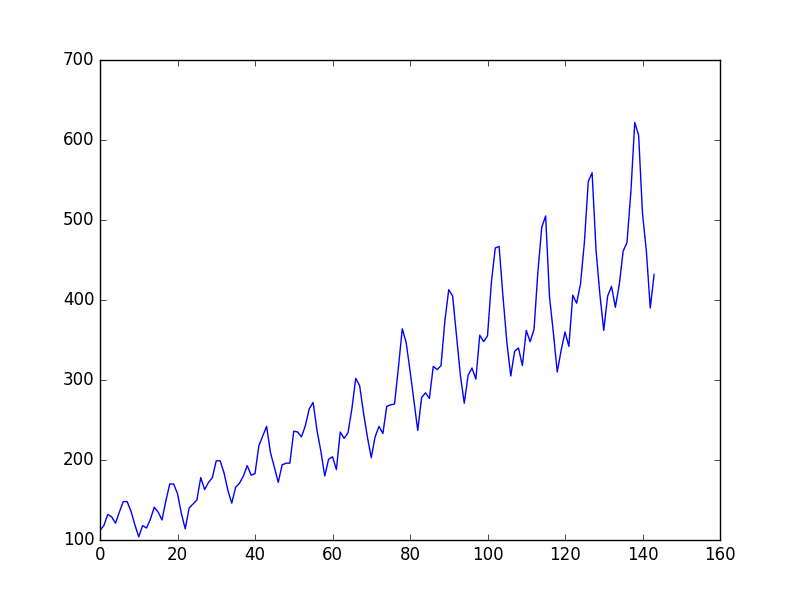
Plot of the airline passengers dataset

Let’s keep things simple and work with the data as-is.

Normally, it is a good idea to investigate various data preparation techniques to rescale the data and make it stationary.

Need help with Deep Learning for Time Series?

Take my free 7-day email crash course now (with sample code).

Click to sign-up and also get a free PDF Ebook version of the course.

Multilayer Perceptron Regression

You want to phrase the time series prediction problem as a regression problem.

That is, given the number of passengers (in units of thousands) this month, what is the number of passengers next month?

You can write a simple function to convert your single column of data into a two-column dataset: the first column containing this month’s (t) passenger count and the second column containing next month’s (t+1) passenger count to be predicted.

Before you get started, let’s first import all the functions and classes you will need to use. This assumes a working SciPy environment with the Keras deep learning library installed.

import numpy as np

import matplotlib.pyplot as plt

import pandas as pd

from tensorflow.keras.models import Sequential

from tensorflow.keras.layers import Dense

You can also use the code from the previous section to load the dataset as a Pandas dataframe. You can then extract the NumPy array from the dataframe and convert the integer values to floating point values, which are more suitable for modeling with a neural network.

...

# load the dataset

dataframe = pd.read_csv('airline-passengers.csv', usecols=[1], engine='python')

dataset = dataframe.values

dataset = dataset.astype('float32')

After you model the data and estimate the skill of your model on the training dataset, you need to get an idea of the skill of the model on new unseen data. For a normal classification or regression problem, you would do this using cross validation.

With time series data, the sequence of values is important. A simple method that you can use is to split the ordered dataset into train and test datasets. The code below calculates the index of the split point and separates the data into the training datasets with 67% of the observations used to train your model, leaving the remaining 33% for testing the model.

...

# split into train and test sets

train_size = int(len(dataset) * 0.67)

test_size = len(dataset) - train_size

train, test = dataset[0:train_size,:], dataset[train_size:len(dataset),:]

print(len(train), len(test))

Now, you can define a function to create a new dataset as described above. The function takes two arguments: the dataset, which is a NumPy array that you want to convert into a dataset, and the look_back, which is the number of previous time steps to use as input variables to predict the next time period, in this case, defaulted to 1.

This default will create a dataset where X is the number of passengers at a given time (t), and Y is the number of passengers at the next time (t + 1).

It can be configured, and you will look at constructing a differently shaped dataset in the next section.

...

# convert an array of values into a dataset matrix

def create_dataset(dataset, look_back=1):

dataX, dataY = [], []

for i in range(len(dataset)-look_back-1):

a = dataset[i:(i+look_back), 0]

dataX.append(a)

dataY.append(dataset[i + look_back, 0])

return np.array(dataX), np.array(dataY)

Let’s take a look at the effect of this function on the first few rows of the dataset.

X Y

112 118

118 132

132 129

129 121

121 135

If you compare these first five rows to the original dataset sample listed in the previous section, you can see the X=t and Y=t+1 pattern in the numbers.

Let’s use this function to prepare the train and test datasets for modeling.

...

# reshape into X=t and Y=t+1

look_back = 1

trainX, trainY = create_dataset(train, look_back)

testX, testY = create_dataset(test, look_back)

We can now fit a Multilayer Perceptron model to the training data.

We use a simple network with one input, one hidden layer with eight neurons, and an output layer. The model is fit using mean squared error, which, if you take the square root, gives you an error score in the units of the dataset.

I tried a few rough parameters and settled on the configuration below, but by no means is the network listed optimized.

...

# create and fit Multilayer Perceptron model

model = Sequential()

model.add(Dense(8, input_shape=(look_back,), activation='relu'))

model.add(Dense(1))

model.compile(loss='mean_squared_error', optimizer='adam')

model.fit(trainX, trainY, epochs=200, batch_size=2, verbose=2)

Once the model is fit, you can estimate the performance of the model on the train and test datasets. This will give you a point of comparison for new models.

...

# Estimate model performance

trainScore = model.evaluate(trainX, trainY, verbose=0)

print('Train Score: %.2f MSE (%.2f RMSE)' % (trainScore, math.sqrt(trainScore)))

testScore = model.evaluate(testX, testY, verbose=0)

print('Test Score: %.2f MSE (%.2f RMSE)' % (testScore, math.sqrt(testScore)))

Finally, you can generate predictions using the model for both the train and test dataset to get a visual indication of the skill of the model.

Because of how the dataset was prepared, you must shift the predictions to align on the x-axis with the original dataset. Once prepared, the data is plotted, showing the original dataset in blue, the predictions for the training dataset in green, and the predictions on the unseen test dataset in red.

...

# generate predictions for training

trainPredict = model.predict(trainX)

testPredict = model.predict(testX)

# shift train predictions for plotting

trainPredictPlot = np.empty_like(dataset)

trainPredictPlot[:, :] = np.nan

trainPredictPlot[look_back:len(trainPredict)+look_back, :] = trainPredict

# shift test predictions for plotting

testPredictPlot = np.empty_like(dataset)

testPredictPlot[:, :] = np.nan

testPredictPlot[len(trainPredict)+(look_back*2)+1:len(dataset)-1, :] = testPredict

# plot baseline and predictions

plt.plot(dataset)

plt.plot(trainPredictPlot)

plt.plot(testPredictPlot)

plt.show()

Tying this all together, the complete example is listed below.

# Multilayer Perceptron to Predict International Airline Passengers (t+1, given t, t-1, t-2)
import numpy as np
import matplotlib.pyplot as plt
from pandas import read_csv
import math
from tensorflow.keras.models import Sequential
from tensorflow.keras.layers import Dense

# convert an array of values into a dataset matrix
def create_dataset(dataset, look_back=1):
	dataX, dataY = [], []
	for i in range(len(dataset)-look_back-1):
		a = dataset[i:(i+look_back), 0]
		dataX.append(a)
		dataY.append(dataset[i + look_back, 0])
	return np.array(dataX), np.array(dataY)

# load the dataset
dataframe = read_csv('airline-passengers.csv', usecols=[1], engine='python')
dataset = dataframe.values
dataset = dataset.astype('float32')
# split into train and test sets
train_size = int(len(dataset) * 0.67)
test_size = len(dataset) - train_size
train, test = dataset[0:train_size,:], dataset[train_size:len(dataset),:]
# reshape dataset
look_back = 3
trainX, trainY = create_dataset(train, look_back)
testX, testY = create_dataset(test, look_back)
# create and fit Multilayer Perceptron model
model = Sequential()
model.add(Dense(12, input_shape=(look_back,), activation='relu'))
model.add(Dense(8, activation='relu'))
model.add(Dense(1))
model.compile(loss='mean_squared_error', optimizer='adam')
model.fit(trainX, trainY, epochs=400, batch_size=2, verbose=2)
# Estimate model performance
trainScore = model.evaluate(trainX, trainY, verbose=0)
print('Train Score: %.2f MSE (%.2f RMSE)' % (trainScore, math.sqrt(trainScore)))
testScore = model.evaluate(testX, testY, verbose=0)
print('Test Score: %.2f MSE (%.2f RMSE)' % (testScore, math.sqrt(testScore)))
# generate predictions for training
trainPredict = model.predict(trainX)
testPredict = model.predict(testX)
# shift train predictions for plotting
trainPredictPlot = np.empty_like(dataset)
trainPredictPlot[:, :] = np.nan
trainPredictPlot[look_back:len(trainPredict)+look_back, :] = trainPredict
# shift test predictions for plotting
testPredictPlot = np.empty_like(dataset)
testPredictPlot[:, :] = np.nan
testPredictPlot[len(trainPredict)+(look_back*2)+1:len(dataset)-1, :] = testPredict
# plot baseline and predictions
plt.plot(dataset)
plt.plot(trainPredictPlot)
plt.plot(testPredictPlot)
plt.show()

# Multilayer Perceptron to Predict International Airline Passengers (t+1, given t, t-1, t-2)

import numpy as np

import matplotlib.pyplot as plt

from pandas import read_csv

import math

from tensorflow.keras.models import Sequential

from tensorflow.keras.layers import Dense

# convert an array of values into a dataset matrix

def create_dataset(dataset, look_back=1):

dataX, dataY = [], []

for i in range(len(dataset)-look_back-1):

a = dataset[i:(i+look_back), 0]

dataX.append(a)

dataY.append(dataset[i + look_back, 0])

return np.array(dataX), np.array(dataY)

# load the dataset

dataframe = read_csv('airline-passengers.csv', usecols=[1], engine='python')

dataset = dataframe.values

dataset = dataset.astype('float32')

# split into train and test sets

train_size = int(len(dataset) * 0.67)

test_size = len(dataset) - train_size

train, test = dataset[0:train_size,:], dataset[train_size:len(dataset),:]

# reshape dataset

look_back = 3

trainX, trainY = create_dataset(train, look_back)

testX, testY = create_dataset(test, look_back)

# create and fit Multilayer Perceptron model

model = Sequential()

model.add(Dense(12, input_shape=(look_back,), activation='relu'))

model.add(Dense(8, activation='relu'))

model.add(Dense(1))

model.compile(loss='mean_squared_error', optimizer='adam')

model.fit(trainX, trainY, epochs=400, batch_size=2, verbose=2)

# Estimate model performance

trainScore = model.evaluate(trainX, trainY, verbose=0)

print('Train Score: %.2f MSE (%.2f RMSE)' % (trainScore, math.sqrt(trainScore)))

testScore = model.evaluate(testX, testY, verbose=0)

print('Test Score: %.2f MSE (%.2f RMSE)' % (testScore, math.sqrt(testScore)))

# generate predictions for training

trainPredict = model.predict(trainX)

testPredict = model.predict(testX)

# shift train predictions for plotting

trainPredictPlot = np.empty_like(dataset)

trainPredictPlot[:, :] = np.nan

trainPredictPlot[look_back:len(trainPredict)+look_back, :] = trainPredict

# shift test predictions for plotting

testPredictPlot = np.empty_like(dataset)

testPredictPlot[:, :] = np.nan

testPredictPlot[len(trainPredict)+(look_back*2)+1:len(dataset)-1, :] = testPredict

# plot baseline and predictions

plt.plot(dataset)

plt.plot(trainPredictPlot)

plt.plot(testPredictPlot)

plt.show()

Running the example reports model performance.

Note: Your results may vary given the stochastic nature of the algorithm or evaluation procedure, or differences in numerical precision. Consider running the example a few times and compare the average outcome.

Taking the square root of the performance estimates, you can see that the model has an average error of 22 passengers (in thousands) on the training dataset and 46 passengers (in thousands) on the test dataset.

...

Epoch 395/400

46/46 - 0s - loss: 513.2617 - 13ms/epoch - 275us/step

Epoch 396/400

46/46 - 0s - loss: 494.1868 - 12ms/epoch - 268us/step

Epoch 397/400

46/46 - 0s - loss: 483.3908 - 12ms/epoch - 268us/step

Epoch 398/400

46/46 - 0s - loss: 501.8111 - 13ms/epoch - 281us/step

Epoch 399/400

46/46 - 0s - loss: 523.2578 - 13ms/epoch - 280us/step

Epoch 400/400

46/46 - 0s - loss: 513.7587 - 12ms/epoch - 263us/step

Train Score: 487.39 MSE (22.08 RMSE)

Test Score: 2070.68 MSE (45.50 RMSE)

From the plot, you can see that the model did a pretty poor job of fitting both the training and the test datasets. It basically predicted the same input value as the output.

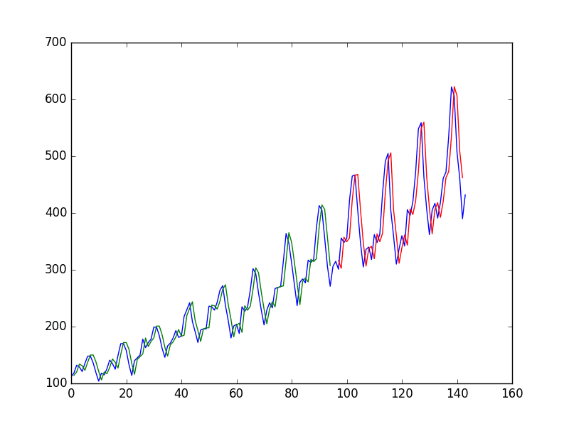
Naive time series predictions with neural network
Blue=whole dataset, Green=training, Red=predictions

Multilayer Perceptron Using the Window Method

You can also phrase the problem so that multiple recent time steps can be used to make the prediction for the next time step.

This is called the window method, and the size of the window is a parameter that can be tuned for each problem.

For example, given the current time (t) to predict the value at the next time in the sequence (t + 1), you can use the current time (t) as well as the two prior times (t-1 and t-2).

When phrased as a regression problem, the input variables are t-2, t-1, and t, and the output variable is t+1.

The create_dataset() function used in the previous section allows you to create this formulation of the time series problem by increasing the look_back argument from 1 to 3.

A sample of the dataset with this formulation looks as follows:

X1 X2 X3 Y

112 118 132 129

118 132 129 121

132 129 121 135

129 121 135 148

121 135 148 148

You can re-run the example in the previous section with the larger window size. You will increase the network capacity to handle the additional information. The first hidden layer is increased to 14 neurons, and a second hidden layer is added with eight neurons. The number of epochs is also increased to 400.

The whole code listing with just the window size change is listed below for completeness.

# load the dataset
dataframe = read_csv('airline-passengers.csv', usecols=[1], engine='python')
dataset = dataframe.values
dataset = dataset.astype('float32')
# split into train and test sets
train_size = int(len(dataset) * 0.67)
test_size = len(dataset) - train_size
train, test = dataset[0:train_size,:], dataset[train_size:len(dataset),:]
# reshape dataset
look_back = 3
trainX, trainY = create_dataset(train, look_back)
testX, testY = create_dataset(test, look_back)
# create and fit Multilayer Perceptron model
model = Sequential()
model.add(Dense(12, input_dim=look_back, activation='relu'))
model.add(Dense(8, activation='relu'))
model.add(Dense(1))
model.compile(loss='mean_squared_error', optimizer='adam')
model.fit(trainX, trainY, epochs=400, batch_size=2, verbose=2)
# Estimate model performance
trainScore = model.evaluate(trainX, trainY, verbose=0)
print('Train Score: %.2f MSE (%.2f RMSE)' % (trainScore, math.sqrt(trainScore)))
testScore = model.evaluate(testX, testY, verbose=0)
print('Test Score: %.2f MSE (%.2f RMSE)' % (testScore, math.sqrt(testScore)))
# generate predictions for training
trainPredict = model.predict(trainX)
testPredict = model.predict(testX)
# shift train predictions for plotting
trainPredictPlot = np.empty_like(dataset)
trainPredictPlot[:, :] = np.nan
trainPredictPlot[look_back:len(trainPredict)+look_back, :] = trainPredict
# shift test predictions for plotting
testPredictPlot = np.empty_like(dataset)
testPredictPlot[:, :] = np.nan
testPredictPlot[len(trainPredict)+(look_back*2)+1:len(dataset)-1, :] = testPredict
# plot baseline and predictions
plt.plot(dataset)
plt.plot(trainPredictPlot)
plt.plot(testPredictPlot)
plt.show()

# Multilayer Perceptron to Predict International Airline Passengers (t+1, given t, t-1, t-2)

import numpy as np

import matplotlib.pyplot as plt

from pandas import read_csv

import math

from tensorflow.keras.models import Sequential

from tensorflow.keras.layers import Dense

# convert an array of values into a dataset matrix

def create_dataset(dataset, look_back=1):

dataX, dataY = [], []

for i in range(len(dataset)-look_back-1):

a = dataset[i:(i+look_back), 0]

dataX.append(a)

dataY.append(dataset[i + look_back, 0])

return np.array(dataX), np.array(dataY)

# load the dataset

dataframe = read_csv('airline-passengers.csv', usecols=[1], engine='python')

dataset = dataframe.values

dataset = dataset.astype('float32')

# split into train and test sets

train_size = int(len(dataset) * 0.67)

test_size = len(dataset) - train_size

train, test = dataset[0:train_size,:], dataset[train_size:len(dataset),:]

# reshape dataset

look_back = 3

trainX, trainY = create_dataset(train, look_back)

testX, testY = create_dataset(test, look_back)

# create and fit Multilayer Perceptron model

model = Sequential()

model.add(Dense(12, input_dim=look_back, activation='relu'))

model.add(Dense(8, activation='relu'))

model.add(Dense(1))

model.compile(loss='mean_squared_error', optimizer='adam')

model.fit(trainX, trainY, epochs=400, batch_size=2, verbose=2)

# Estimate model performance

trainScore = model.evaluate(trainX, trainY, verbose=0)

print('Train Score: %.2f MSE (%.2f RMSE)' % (trainScore, math.sqrt(trainScore)))

testScore = model.evaluate(testX, testY, verbose=0)

print('Test Score: %.2f MSE (%.2f RMSE)' % (testScore, math.sqrt(testScore)))

# generate predictions for training

trainPredict = model.predict(trainX)

testPredict = model.predict(testX)

# shift train predictions for plotting

trainPredictPlot = np.empty_like(dataset)

trainPredictPlot[:, :] = np.nan

trainPredictPlot[look_back:len(trainPredict)+look_back, :] = trainPredict

# shift test predictions for plotting

testPredictPlot = np.empty_like(dataset)

testPredictPlot[:, :] = np.nan

testPredictPlot[len(trainPredict)+(look_back*2)+1:len(dataset)-1, :] = testPredict

# plot baseline and predictions

plt.plot(dataset)

plt.plot(trainPredictPlot)

plt.plot(testPredictPlot)

plt.show()

Running the example provides the following output.

Epoch 395/400

46/46 - 0s - loss: 419.0309 - 14ms/epoch - 294us/step

Epoch 396/400

46/46 - 0s - loss: 429.3398 - 14ms/epoch - 300us/step

Epoch 397/400

46/46 - 0s - loss: 412.2588 - 14ms/epoch - 298us/step

Epoch 398/400

46/46 - 0s - loss: 424.6126 - 13ms/epoch - 292us/step

Epoch 399/400

46/46 - 0s - loss: 429.6443 - 14ms/epoch - 296us/step

Epoch 400/400

46/46 - 0s - loss: 419.9067 - 14ms/epoch - 301us/step

Train Score: 393.07 MSE (19.83 RMSE)

Test Score: 1833.35 MSE (42.82 RMSE)

You can see that the error was not significantly reduced compared to that of the previous section.

Looking at the graph, you can see more structure in the predictions.

Again, the window size and the network architecture were not tuned; this is just a demonstration of how to frame a prediction problem.

Taking the square root of the performance scores, you can see the average error on the training dataset was 20 passengers (in thousands per month), and the average error on the unseen test set was 43 passengers (in thousands per month).

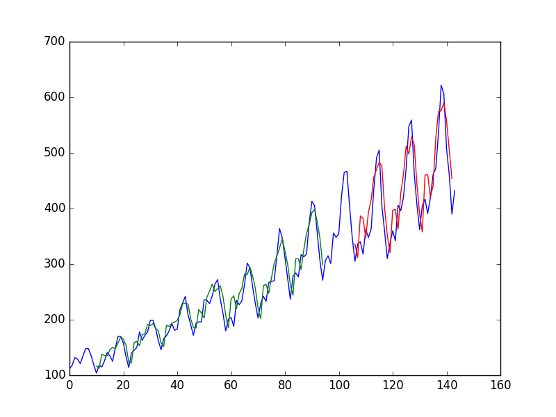
Window method for time series predictions with neural networks
Blue=whole dataset, Green=training, Red=predictions

Summary

In this post, you discovered how to develop a neural network model for a time series prediction problem using the Keras deep learning library.

After working through this tutorial, you now know:

About the international airline passenger prediction time series dataset
How to frame time series prediction problems as regression problems and develop a neural network model
How to use the window approach to frame a time series prediction problem and develop a neural network model

Do you have any questions about time series prediction with neural networks or this post?
Ask your question in the comments below, and I will do my best to answer.

234 Responses to Time Series Prediction with Deep Learning in Keras

Steve Buckley August 13, 2016 at 2:12 am #

Hi Jason,

This is a new tool for me so an interesting post to get started!

It looks to me like your plot for the first method is wrong. As you’re only giving the previous time point to predict the next, the model is going to fit (close to) a straight line and won’t pull out the periodicity your plot suggests. The almost perfect fit of the red line to the blue line also doesn’t reflect the much worse fit suggested in the model score!

Hope that’s helpful.

Reply
Curious George August 17, 2016 at 2:29 am #

Hi Jason,

How can you use this technique to forecast into the future?

Thanks!

Reply
- Jason Brownlee August 17, 2016 at 9:52 am #
  
  This example is forecasting t+1 in the future.
  
  Reply
  - Curious George August 25, 2016 at 1:18 am #
    
    In order to forecast t+2, t+3, t+n…., is it recommended to use the previous prediction (t+1) as the assumed data point.
    
    For example, if I wanted to forecast t+2, I would use the available data including my prediction at t+1.
    
    I understand that the error would increase the further out the forecast due to relying on predictions as data points.
    
    Thoughts?
    
    Reply
    - Jason Brownlee August 25, 2016 at 5:05 am #
      
      Yes, using this approach will provide multiple future data points. As you suggest, the further in the future you go, the more likely errors are to compound.
      
      Give it a go, it’s good to experiment with these models and see what they are capable of.
      
      Reply
  - Curious George August 25, 2016 at 1:51 am #
    
    Also, when running the full code snippet using the window method, the graph produced does not match the one shown.
    
    This is what I’m getting
    
    http://imgur.com/a/NaoYE
    
    Reply
    - Jason Brownlee August 25, 2016 at 5:06 am #
      
      I did update the plotting code with a minor change and did not update the images accordingly. I will update them ASAP.
      
      Reply
  - Andy March 1, 2017 at 6:03 am #
    
    Could you show an example where maybe there was a couple more features. So, say you wanted to predict how many passengers, and you knew about temperature and day of the week (Mon-Sun).
    
    Reply
    - Jason Brownlee March 1, 2017 at 8:46 am #
      
      Hi Andy,
      
      Yes, I am working on more sophisticated time series tutorials at the moment, they should be on the blog soon.
      
      Reply
      - Soren Pallesen June 9, 2017 at 6:18 pm #
        
        Look forward to these time series forecast with multiple features examples – when do you expect to post them to your blog?
        
        As always thx for this valuable resource and for sharing your experience !
      - Jason Brownlee June 10, 2017 at 8:19 am #
        
        Perhaps a month. No promises. I am taking my time to ensure they are good.
  - Ramzan Shahid November 10, 2017 at 4:51 am #
    
    Sir please, share some tutorial on tensorflow and what are the differences to make models in tensorflow and keras. thanks
    
    Reply
    - Jason Brownlee November 10, 2017 at 10:41 am #
      
      Tensorflow is like coding in assembly, Keras is like coding in Python.
      
      Keras is so much simpler and makes you more productive, but gives up some speed and flexibility, a worthy trade-off for most applications.
      
      Reply
  - shahid January 17, 2018 at 6:06 am #
    
    sir can you have done any example for more than one column for time series prediction like stock data? If yes, please share the link of that. Thanks
    
    Reply
    - Jason Brownlee January 17, 2018 at 10:00 am #
      
      See here:
      https://machinelearningmastery.com/multivariate-time-series-forecasting-lstms-keras/
      
      Reply
      - poiuwn September 8, 2018 at 4:53 pm #
        
        Super! Will take some time on it soon. Thanks so much, Jason!
Keshav Mathur August 30, 2016 at 7:20 am #

Hello,

Thank you for a great article. I have a big doubt and also related to the plot posted in the earlier comment which shows a sort of lag in the prediction. Here we are training the model on t to get predictions for t+1.

Given this I would assume that when the model sees an input of 112 it should predict around 118 (first data point in the training set). But that’s not what the predictions show. Copying the top 5 train points and their subsequent predictions generated by the code given in this post for the first example:

trainX[:5] trainPredict[:5]
[ 112.], [112.56],
[ 118.], [118.47],
[ 132.], [132.26],
[ 129.], [129.55],
[ 121.] [121.57],

I am trying to understand from a model perspective as to why is it predicting with a lag?

Reply
- Jason Brownlee October 9, 2016 at 10:54 am #
  
  Thanks Keshav, I have updated the description and the graphs.
  
  Reply
Jev September 5, 2016 at 7:17 am #

Just as Steve Buckley pointed out, your first method seems to be wrong. The model indeed just fits a straight line ( yPred = a*X+b) , which can be verified by calculating predictions on an input such as arange(200).
Because you shift the results afterwards before plotting, the outcome seems very good. However, from a conceptual point of view, it should be impossible to predict X_t+1 correctly based on only X_t, as the latter contains no trend or seasonal information.

Here is what I’ve got after trying to reproduce your results:

X Y yPred
0 112.0 118.0 112.897537
1 118.0 132.0 118.847107
2 132.0 129.0 132.729446
3 129.0 121.0 129.754669
….

as you can see, the yPred is way off ( it should be equal to Y), but looks good when shifted one period.

Reply
- Jason Brownlee October 9, 2016 at 10:55 am #
  
  Yep, right on Jev, thanks. I have updated the description and the graphs.
  
  Reply
Max Clayer September 14, 2016 at 4:01 am #

Hi, Jason

I also have to agree with Jev, I would expect using predict(trainX) would give values closer to trainY values not trainX values.

Reply
- Jason Brownlee October 9, 2016 at 10:56 am #
  
  They do Max, you’re right. I have updated the graphs to better reflect the actual predictions made.
  
  Reply
Himadri September 24, 2016 at 11:56 pm #

Hi Jason,
Thanks for such a wonderful tutorial!
I was just wondering if in function create_dataset, there should be range(len(dataset)-1) in the loop. Hence for plotting logic, it should be:

…
trainPredictPlot[lb:len(train),:] = trainPredict
…
testPredictPlot[len(train)+lb:len(dataset),:] = testPredict

I am just in a big confusion with the index and getting somewhat difference plot for look_back=3 : http://imgur.com/a/DMbOU

Reply
Veltzer Doron September 26, 2016 at 6:06 pm #

Hey, thanks for a most helpful tutorial, any ideas why this seems to work better than the time series predictions using RNNs and LSTM in the sister tutorial? My intuition predicts the opposite.

Reply
- Jason Brownlee September 27, 2016 at 7:41 am #
  
  I’m glad you like it Veltzer.
  
  Great question, the LSTMs probably require more fine tuning I expect.
  
  Reply
  - Tamil March 29, 2021 at 1:13 pm #
    
    trainPredictPlot = numpy.empty_like(dataset)
    trainPredictPlot[:, :] = numpy.nan
    trainPredictPlot[look_back:len(trainPredict)+look_back, :] = trainPredict
    # shift test predictions for plotting
    testPredictPlot = numpy.empty_like(dataset)
    testPredictPlot[:, :] = numpy.nan
    testPredictPlot[len(trainPredict)+(look_back*2)+1:
    I need an explanation for this part of coding
    Can anyone please explain
    
    Reply
    - Jason Brownlee March 30, 2021 at 5:56 am #
      
      From memory, it creates a line plot of the training dataset followed by the predictions of the test dataset.
      
      It’s a terrible implementation, there are much simpler ways to do this now.
      
      Reply
Newbtothis September 29, 2016 at 12:02 pm #

Hey there! Great blog and articles – the examples really help a lot! I’m new to this so excuse the stupid question if applicable – I want to predict the next three outputs based on the same input. Is that doable in the LSTM framework? This is for predicting the water temperature for the next 3 days.

Reply
- Jason Brownlee September 30, 2016 at 7:48 am #
  
  Yes, this is called sequence to sequence prediction.
  
  I see two main options:
  
  – Run the LSTM 3 times and feed output as input.
  – Change the LSTM to output 3 numbers.
  
  Reply
Han September 30, 2016 at 11:37 am #

This particular time-series has strong seasonality and looks exponential in trend. In reality, the growth rate of this time series is more important. Could you plot the year-on-year growth rate?

Reply
- Jason Brownlee October 1, 2016 at 8:00 am #
  
  There would be benefit in modeling a stationary version of the data, I agree.
  
  Reply
Han October 1, 2016 at 2:44 am #

I agree with Steve Buckley. The code is predicting x[i+1] = x[i] (approximately), that why the last part of code, which is supposed to fix the shift, couldn’t get the shift part right.

Try the following: pick any point in your testX, say testX[i], use the model to predict testY[i], then instead of using testX[i+1], use testY[i] as the input parameter for model.predict(), and so on. You will end up with a nearly straight line.

I’d thank you for your wonderful posts on neural network, which helped me a lot when learning neural network. However, this particular code is not correct.

Reply
Jeremy October 5, 2016 at 1:58 pm #

Thanks for great article! It is really helpful for me. I have one question. If I have two more variable, how can i do? Take example, my data looks like follow,
date windspeed rain price
20160101 10 100 1000
20160102 10 80 1010
…
I’d like to predict the price.

Reply
- Jason Brownlee October 6, 2016 at 9:26 am #
  
  Hi Jeremy, each input would be a feature. You could then use the window method to frame multiple time steps of multiple features as new features.
  
  For example:
  
  x1(t), x2(t), x1(t-1), x2(t-1) to predict y(t+1)
  
  1
  
  x1(t), x2(t), x1(t-1), x2(t-1) to predict y(t+1)
  
  Reply
  - Shimin November 22, 2016 at 10:53 pm #
    
    Hi Jason,
    
    Thanks for your great explanation!
    
    I have one question like Jeremy’s. Is there any suggestion for me if I want to predict 2 variables? Data frame shown as below:
    
    Date X1 X2 X3 X4 Y1 Y2
    
    I want to predict Y1 and Y2. Also, Y1 and Y2 have some correlations.
    
    Reply
    - Jason Brownlee November 23, 2016 at 8:59 am #
      
      hi Shimin,
      
      Yes, this is often called a sequence prediction problem in deep learning or a multi-step prediction problem in time series prediction.
      
      You can use an LSTM with two outputs or you can use an MLP with two outputs to model this problem. Be sure to prepare your data into this form.
      
      I hope that helps.
      
      Reply
Sunny October 18, 2016 at 9:09 am #

Jason,
Great writeup on using Keras for TS data. My dataset is something like below:# print the

Date Time Power1 Power2 Power3 Meter1 Meter2
12/02/2012 02:53:00 2.423 0.118 0.0303 0.020 1.1000

My feature vectors/predictors are Date, Time, Power1, Power2, Power3, Meter1. i am trying to predict Meter 2.

I would like to instead of using MLP use RNN/LSTM for the above time series prediction.
Can you pl. suggest is this is possible? and if yes, any pointers would help
thanks
Sunny

Reply
- Jason Brownlee October 19, 2016 at 9:10 am #
  
  Hi Sunny, this tutorial will help to get you started:
  https://machinelearningmastery.com/time-series-prediction-lstm-recurrent-neural-networks-python-keras/
  
  Reply
nicoad October 31, 2016 at 7:52 pm #

Hello , nice tutorial .

I have one question : it would be usefull to have similar stuff on live data. let s say I have access to some real time data (software downloads, stock price …) , would it requires to train the model each time new data is available ?

Reply
- Jason Brownlee November 1, 2016 at 7:59 am #
  
  I agree nicoad, a real-time example would be great. I’ll look into it.
  
  A great thing about neural networks is that they can be updated with new data and do not have to be re-trained from scratch.
  
  Reply
sherlockatszx November 8, 2016 at 3:36 am #

Hi,your original post code is to use 1(or 3) dimension X to predict the later 1 dimension Y.how about I want to use 48 dimension X to predict 49th and 50th.what i mean is i increase the time unit i want to predict ,predict 3 or even 10 time unit . under such condition : does that mean i just change the output_dime of the last output layer :

model.add(Dense(
output_dim=3))

Is that right?

Reply
- Jason Brownlee November 8, 2016 at 9:58 am #
  
  Yes, that looks right. Let me know how you go.
  
  Reply
  - sherlockatszx November 8, 2016 at 6:56 pm #
    
    Hi jason, I make a quick expriment in jupyter notebook and published in the github
    github:https://github.com/sherlockhoatszx/TimeSeriesPredctionUsingDeeplearning
    the code could work.
    However If you look very carefully of the trainPredict data(IN[18] of the notebook).
    
    the first 3 array is:
    array([[ 128.60112 , 127.5030365 ],
    [ 121.16256714, 122.3662262 ],
    [ 144.46884155, 145.67802429]
    
    the list inside [ 128.6,127.5 ] [121,2,122,3] does not like t+1 and t+2.
    **Instead,** It looks like 2 probaly prediction for 1 unit.
    What i means is [128.6,127.5] doesn’t mean t+1 and t+2 prediction, it most possibly mean 2 possible prediction for t+1.
    one output cell with 2dimension and 2 output cell with 1 dimension is different.
    I discussed it with other guy in github .
    https://github.com/Vict0rSch/deep_learning/issues/11
    It seems i should use seq2seq or use timedistributed wrapper .
    
    I stilll explored this and have not got one solution .
    
    What is your suggestion?
    
    Reply
    - Jason Brownlee November 9, 2016 at 9:49 am #
      
      That does sound like good advice. Treat the problem as sequence to sequence problem.
      
      Reply
sherlockatszx November 8, 2016 at 8:28 pm #

hi jason , I made a experiment on the jupyter notebook and published on the github .The code could output 2 columns data.
https://github.com/sherlockhoatszx/TimeSeriesPredctionUsingDeeplearning/blob/master/README.md

However! If you look very carefully of the trainPredict data(IN[18] of the notebook).

the first 3 array is:
array([[ 128.60112 , 127.5030365 ],
[ 121.16256714, 122.3662262 ],
[ 144.46884155, 145.67802429]

the list inside [ 128.6,127.5 ] [121,2,122,3] does not like t+1 and t+2.
**Instead,** It looks like 2 probaly prediction for 1 unit.
What i means is [128.6,127.5] doesn’t mean t+1 and t+2 prediction, it most possibly mean 2 possible prediction for t+1.
1 output cell with 2 dimension and 2 output cell with 1 dimension is different.
The input dimension and the output dimension will be tricky for the NN.

Reply
Xiao November 16, 2016 at 1:59 am #

Thanks Jason for the conceptual explaining. I have one question about the KERAS package:

It looks you input the raw data (x=118 etc) to KERAS. Do you know whether KERAS needs to standardize (normalize) the data to (0,1) or (-1,1) or some distribution with mean of 0?

— Xiao

Reply
- Jason Brownlee November 16, 2016 at 9:32 am #
  
  Great question Xiao,
  
  It is a good idea to standardize data or normalize data when working with neural networks. Try it on your problem and see if it affects the performance of your model.
  
  Reply
  - Satoshi Report November 19, 2016 at 2:24 pm #
    
    Wasn’t the data normalized in an early version of this post?
    
    Reply
    - Jason Brownlee November 22, 2016 at 6:46 am #
      
      I don’t believe so Satoshi.
      
      Normalization is a great idea in general when working with neural nets, though.
      
      Reply
charith December 12, 2016 at 8:11 pm #

I keep getting this error dt = datetime.datetime.fromordinal(ix).replace(tzinfo=UTC)

ValueError: ordinal must be >= 1

Reply
- Jason Brownlee December 13, 2016 at 8:05 am #
  
  Sorry charith, I have not seen this error before.
  
  Reply
Trex January 7, 2017 at 8:07 am #

In Your text you say, the window size is 3, But in Your Code you use loop_back = 10 ?

Reply
- Jason Brownlee January 7, 2017 at 8:41 am #
  
  Thanks Trex.
  
  That is a typo from some experimenting I was doing at one point. Fixed.
  
  Reply
Trex January 7, 2017 at 11:44 am #

No problem,

I have another question:

what the algorithm now does is predict 1 value. I want to predict with this MLP like n-values.

How should this work?

Reply
- Jason Brownlee January 8, 2017 at 5:17 am #
  
  Reframe your training dataset to match what you require and change the number of neurons in the output layer to the number of outputs you desire.
  
  Reply
Mansolo January 7, 2017 at 12:47 pm #

Hey Sir,

great Tutorial.

I am trying to build a NN for Time-Series-Prediction. But my Datas are different than yours.

I want to predict a whole next day. But a whole day is defined as 48 values.

Some lines of the Blank datas:
2016-11-10 05:00:00.000 0
2016-11-10 05:30:00.000 0
2016-11-10 06:00:00.000 1
2016-11-10 06:30:00.000 3
2016-11-10 07:00:00.000 12
2016-11-10 07:30:00.000 36
2016-11-10 08:00:00.000 89
2016-11-10 08:30:00.000 120
2016-11-10 09:00:00.000 209
2016-11-10 09:30:00.000 233
2016-11-10 10:00:00.000 217
2016-11-10 10:30:00.000 199
2016-11-10 11:00:00.000 244

There is a value for each half an hour of a whole day.

i want to predict the values for every half an hour for the next few days. How could this work?

Reply
Hem January 8, 2017 at 3:43 pm #

Could you do an example for a Multivariate Time Series? 🙂

Reply
- Jason Brownlee January 9, 2017 at 7:48 am #
  
  Yes, there are some tutorials scheduled on the blog. I will link to them once they’re out.
  
  Reply
Bonje January 12, 2017 at 12:19 am #

Why doesnt need the reLu Activation function that the input datas are normalized between 0 and 1?

If i use the sigmoid activation function, there is a must, that the input datas are normalized.

But why reLu doesnt need that?

Reply
- Jason Brownlee January 12, 2017 at 9:28 am #
  
  Generally, because of the bounds of the sigmoid function imposes hard limits values outside of 0-1.
  
  The Rectifier function is quite different, you can read up on it here:
  https://en.wikipedia.org/wiki/Rectifier_(neural_networks)
  
  I’d recommend implementing in excel or Python and having a play with inputs and outputs.
  
  Reply
Bonje January 12, 2017 at 1:10 am #

Another Question:

Your Input Layer uses reLu as activition Function.
But why has your Output Layer no activition Function? Is there a default activition function which keras uses if you give one as parameter? if yes, which is it? if no, why is it possible to have a Layer without a activition function in it?

Thanks 🙂

Reply
- Jason Brownlee January 12, 2017 at 9:31 am #
  
  Yes the default is Linear, this is a desirable activation function on regression problems.
  
  Reply
Bonje January 12, 2017 at 1:11 am #

dont give one as parameter*

Reply
Dmitry N. Medvedev February 4, 2017 at 1:11 pm #

A stupid question, sir.

Suppose I have a dataset with two fields: “date” (timestamp), “amount” (float32) describing a year.

on the first day of each month the amount is set to -200.

This is true for 11 months, except for the 12th (December).

Is there a way to train a NN so that it returns 12, marking the December as not having such and amount on its first day?

Reply
- Jason Brownlee February 5, 2017 at 5:15 am #
  
  Sorry Dmitry, I’m not sure I really understand your question.
  
  Perhaps you’re able to ask it a different way or provide a small example?
  
  Reply
Thomas Durant February 9, 2017 at 3:36 pm #

Is it common to only predict the single next time point? Or are there times/ways to predict 2,3, and 4 times points into the future, and if so, how do you assess performance metrics for those predictions?

Reply
- Jason Brownlee February 10, 2017 at 9:50 am #
  
  Good question Thomas.
  
  The forecast time horizon is problem specific. You can predict multiple steps with a MLP or LSTM using multiple neurons in the output layer.
  
  Evaluation is problem specific but could be RMSE across the entire forecast or per forecast lead time.
  
  Reply
zhou February 28, 2017 at 8:34 pm #

thanks for Jason’s post, I benefit a lot from it. now I have a problem:how can I get the passengers in 1961-01? anticipates your reply.

Reply
- Jason Brownlee March 1, 2017 at 8:36 am #
  
  You can train your model on all available data, then call model.predict() to forecast the next out of sample observation.
  
  Reply
  - zhou March 3, 2017 at 1:42 pm #
    
    it seems the model can’t forecast the next month in future？
    
    Reply
    - Jason Brownlee March 6, 2017 at 10:41 am #
      
      What do you mean exactly zhou?
      
      Reply
      - zhou March 8, 2017 at 4:39 pm #
        
        sorry. I want to forecast the passengers in future, what should I do?
Viktor March 2, 2017 at 12:08 am #

Thanks for the tutorial, Jason. it’s very useful. It would be nice to also know how you chose the different parameters for MLP, and you’d go about optimizing them.

Reply
- Jason Brownlee March 2, 2017 at 8:17 am #
  
  Thanks Viktor, I hope to cover more tutorials on this topic.
  
  You can see this post on how to best tune an MLP:
  https://machinelearningmastery.com/improve-deep-learning-performance/
  
  Reply
0xKA March 6, 2017 at 7:35 pm #

In the first case. If I shift model to the left side, it will be a good model for forecasting because predicted values are quite fit the original data. Is it possible to do that ?

Reply
- Jason Brownlee March 7, 2017 at 9:35 am #
  
  Can you give an example of what you mean?
  
  Reply
Sphurti March 22, 2017 at 4:29 pm #

Is there any specific condition to use activation functions? how to deside which activation function is more suitable for linear or nonlinear datasets?

Reply
- Jason Brownlee March 23, 2017 at 8:47 am #
  
  There are some rules.
  
  Relu in hidden because it works really well. Sigmoid for binary outputs, linear for regression outputs, softmax for muti-class classification.
  
  Often you can transform your data for the bounds of a given activation function (e.g. 0,1 for sigmoid, -1,1 for tanh, etc.)
  
  I hope that helps as a start.
  
  Reply
  - Sphurti March 23, 2017 at 5:51 pm #
    
    how to decide the optimizer? Is there any relevance with activation function?
    
    Reply
    - Jason Brownlee March 24, 2017 at 7:53 am #
      
      Not really. It’s a matter of taste it seems (speed vs time).
      
      Reply
John March 29, 2017 at 1:37 am #

What kind of validation are you using in this tutorial? is it cross validation?

Reply
- Jason Brownlee March 29, 2017 at 9:08 am #
  
  No, a train-test split.
  
  Reply
Sphurti March 29, 2017 at 3:31 pm #

Is there any another deep learning algorithms that can be used for time series prediction? why to prefer multilayer perceptron for time series prediction?

Reply
- Jason Brownlee March 30, 2017 at 8:47 am #
  
  Yes, you can use Long Short-Term Memory (LSTM) networks.
  
  Reply
Qiushi Wang April 3, 2017 at 5:22 pm #

Hi Jason,

I always have a question, if we only predict 1 time step further (t+1), the accurate predicted result is just copy the value of t, as the first figure shows. When we add more input like (t-2, t-1, t), the predicted result get worse. Even compare with other prediction method like ARIMA, RNN, this conclusion perhaps is still correct. To better exhibit the power of these prediction methods, should we try to predict more time steps further t+2, t+3, …?

Thanks

Reply
- Jason Brownlee April 4, 2017 at 9:13 am #
  
  It is a good idea to make the input data stationary and scale it. Then the network needs to be tuned for the problem.
  
  Reply
Stephan Oelze April 10, 2017 at 1:56 am #

Dear Jason.

Thanks for sharing your information here. Anyway i was not able to reproduce your last figure. On my machine it still looks like the “bad” figure.

https://www2.pic-upload.de/img/32978063/auto.png

I used the code as stated above. Where is my missunderstanding here?

https://pastebin.com/EzvjnvGv

Thank You!
silly me 🙂

Reply
- Jason Brownlee April 10, 2017 at 7:38 am #
  
  Perhaps try fitting the network for longer?
  
  Reply
trupti April 11, 2017 at 3:22 pm #

thanks for this post..actually I am referring this for my work. my dataset is linear. Can I use softplus or elu as an activation function for linear data?

Reply
- Jason Brownlee April 12, 2017 at 7:50 am #
  
  Yes, but your model may be more complex than is needed. In fact, you may be better off with a linear model like Linear Regression or Logistic Regression.
  
  Reply
ikok April 20, 2017 at 8:31 am #

Firstly thanks Jason, I try MLP and LSTM based models on my time series data, and I get some RMSE values. ( e.g. train rmse 10, and test 11) (my example count 1400, min value:21, max value 210 ) What is acceptance value of RMSE. ?

Reply
- Jason Brownlee April 20, 2017 at 9:35 am #
  
  Nice work!
  
  An acceptable RMSE depends on your problem and how much error you can bear.
  
  Reply
Dmitry April 21, 2017 at 6:58 pm #

Great article, thank you.
Is it possible to make a DNN with several outputs? For example the output layer has several neurons responsible for different flight directions. What difficulties can arise?

Reply
- Jason Brownlee April 22, 2017 at 9:25 am #
  
  Yes, try it.
  
  Skill at future time steps often degrades quickly.
  
  Reply
piemonsparrow April 21, 2017 at 10:50 pm #

Hello, Jason, i am a student, recently i am learning from your blog. Could you make a display deep learning model training history in this article? I will be very appreciated if you can, because i am a newer. Thank you!

Reply
- Jason Brownlee April 22, 2017 at 9:26 am #
  
  This example shows you how to display training history:
  https://machinelearningmastery.com/display-deep-learning-model-training-history-in-keras/
  
  Reply
Hans April 23, 2017 at 2:09 pm #

Does anybody have an idea/code snippet how to store observations of this example code in a variable, so that the variable can be used to to make predictions beyond the airline dataset (one step in the future)?

Reply
Hans April 24, 2017 at 3:20 pm #

Would it be logical incorrect to extend the testX-Array with for example [0,0,0] to forecast unseen data/ a step in the future?

Reply
- Jason Brownlee April 25, 2017 at 7:45 am #
  
  It would not be required.
  
  Fit your model on all available data. When a new observation arrives, scale it appropriately, gather it with the other lag observations your model requires as input and call model.predict().
  
  Reply
Hans April 24, 2017 at 4:45 pm #

Is there a magic trick to get the right array-format for a prediction based on observations?
I always get the wrong format:

obsv1 = testPredict[4] obsv2 = testPredict[5] obsv3 = testPredict[6]
dataset = obsv1, obsv2, obsv3 dataX = [] dataX.append(dataset) #dataX.append(obsv2) #dataX.append(obsv3) myNewX = numpy.array(dataX)

Reply
- Hans April 24, 2017 at 5:05 pm #
  
  Update:
  
  After several days I manged to make a prediction on unseen data in this example (code below).
  Is this way correct?
  How many observations should be used to get a good prediction on unseen data.
  Are there standard tools available to measure corresponding performances and suggest the amount of observations?
  Would this topic the same as choosing the right window-size for time-series analysis, or where would be the difference?
  
  Code:
  
  obsv1 = float(testPredict[4])
  obsv2 = float(testPredict[5])
  obsv3 = float(testPredict[6])
  
  dataX = []
  myNewX = []
  dataX.append(obsv1)
  dataX.append(obsv2)
  dataX.append(obsv3)
  myNewX.append(dataX)
  myNewX = numpy.array(myNewX)
  
  futureStepPredict = model.predict(myNewX)
  print(futureStepPredict)
  
  Reply
  - Jason Brownlee April 25, 2017 at 7:48 am #
    
    Looks fine.
    
    The number of obs required depends on how you have configured your model.
    
    The “best” window size for a given problem is unknown, you must discover it through trial and error, see this post:
    https://machinelearningmastery.com/a-data-driven-approach-to-machine-learning/
    
    Reply
    - Hans April 28, 2017 at 1:04 pm #
      
      Is there a method or trial and error-strategy to find out how many lag observations are ‘best’ for a forecast of unseen data?
      Is there a relation between look_back (window size) and lag observations?
      In theory I could use all observations to predict one step of unseen data. Would this be useful?
      
      Reply
      - Jason Brownlee April 29, 2017 at 7:20 am #
        
        Look-back defines the lag.
        
        You can use ACF and PACF plots to discover the most relevant lag obs:
        https://machinelearningmastery.com/gentle-introduction-autocorrelation-partial-autocorrelation/
        
        The “promise” of LSTMs is that they can learn the appropriate time dependence structure without having it explicitly specified.
  - Hans May 31, 2017 at 8:38 pm #
    
    If I fill the model with 3 obs, I get 3 predictions/data points of unseen data.
    
    If I only want to predict one step in the future, should I build an average of the resulting 3 predictions,
    or should I simply use the last of the 3 prediction steps?
    
    Thank you.
    
    Reply
    - Jason Brownlee June 2, 2017 at 12:46 pm #
      
      I would recommend changing the model to make one prediction if only one time step prediction is required.
      
      Reply
      - Hans June 2, 2017 at 7:49 pm #
        
        How would you change the Multilayer Perceptron model of this site in this regard?
  - Hans June 9, 2017 at 9:04 pm #
    
    I have a misconception here. Don’t do the same fellow reader!
    
    With “obsv(n) = float(testPredict[n])” I took predictions of the test dataset as observations.
    
    THAT’S WRONG!
    
    Instead we take a partition of the original raw data as x/observations to predict unseen data, with a trained/fitted model- IN EVERY CASE.
    
    Like in R:
    https://machinelearningmastery.com/finalize-machine-learning-models-in-r/#comment-401949
    
    Is this right Jason?
    
    Reply
- Jason Brownlee April 25, 2017 at 7:46 am #
  
  If you need a 2D array with 1 row and 2 columns, you can do something like:
  
  data = [0.1, 0.1] data = numpy.array(data) data = data.resize(1, 2)
  
  1
  2
  3
  
  data = [0.1, 0.1]
  data = numpy.array(data)
  data = data.resize(1, 2)
  
  Reply
Md. Armanur Rahman April 28, 2017 at 2:48 pm #

Hello Sir,

This is Arman from Malaysia. I am a student of Multimedia University. I want to do “Self-Tuning performance of Hadoop using Deep Learning”. So which framework I will consider for this sort of problem. as like DBM, DBN , CNN, RNN ?

I need your suggestion.

With best regards
Arman

Reply
- Jason Brownlee April 29, 2017 at 7:21 am #
  
  I would recommend following this process:
  https://machinelearningmastery.com/start-here/#process
  
  Reply
Hans May 1, 2017 at 6:41 pm #

Are there any more concerns about this code. Or is it updated and technical correct now?

Reply
- Jason Brownlee May 2, 2017 at 5:57 am #
  
  We can always do things better.
  
  For this example, I would recommend exploring providing the data as time steps and explore larger networks fit for more epochs.
  
  Reply
  - Hans May 2, 2017 at 11:31 pm #
    
    Hm, I’m not sure if I understand it right.
    
    I believe I’m already feeding it with time-step like so:
    
    return datetime.strptime(x, ‘%Y-%m-%d’)
    
    My raw data items have a decent date column. Is this what you meant?
    
    How do we explore larger networks fit for more epochs?
    
    I have everything parameterized in a central batch file now (pipeline).
    
    Should I increase the epochs for…
    
    model.fit(trainX, trainY, epochs=myEpochs, batch_size=myBatchSize, verbose=0)
    
    Thank you.
    
    Reply
Hans May 1, 2017 at 6:58 pm #

I’m trying to adapt some code from:

https://machinelearningmastery.com/time-series-forecasting-long-short-term-memory-network-python/

…and build the variable EXPECTED in the context of this script.
Unfortunately I don’t know how to do it right. I’m a little bit frustrated at this point.

for i in range(len(test)): <-- what should I better use here? expected = dataset[len(train) + i + 1] <-- what should I better use here? print(expected)
This looks cool so far, could I use the index to retrieve a var called EXPECTED?
for i in range(len(testPredict)): pre = '%.3f' % testPredict[i] print(pre)

A code example would help to solve my index-confusions.

Reply
Stefan June 15, 2017 at 2:06 am #

This is a great example that machine learning is often much more than knowing how to use the algorithms / libraries. It’s always important to understand the data we are working with. For this example as it is 1 dimensional this is luckily quite easily done.
In the first example we are giving the the algorithm one previous value and ask it “What will the next value be?”.

Since we use a neural net not taking into account any time behavior, this system is strongly overdetermined. There are a lot of values at the y value 290 for example. For half of them the values decline, for half of them the values increase. If we don’t give the algorithm any indication, how should it know which direction this would be for the test datapoint? There is just not enough information.

One idea could be to additionally give the algorithm the gradient which would help in the decision whether we a rising or a falling value follows (which is somehow what we do when adding a lookback of 2). Yet, the results do obviously not improve significantly.

Here I want to come back to “understand the data you are dealing with”. If we look at the plot, there are two characteristics which are obvious. A generally rising trend and a periodicity. We want the algorithm to cover both. Only then, will the prediction be accurate. We see that there is an obvious 12 month periodicity (think of summer vacation, christmas). If we want the algorithm to cover that periodicity without including model knowledge (as we are using an ANN) we have to at least provide it the data in a format to deduct this property.

Hence: Extending the lookback to 12 month (12 datapoints in the X) will lead to a significantly improved “1 month ahead”-prediction! Now however, we have a higher feature dimension, which might not be desired due to computational reasons (doesn’t matter for this toy example, but anyway…). Next thing we do is take only 3 month steps at lookback (still look back 12 month but skip 2 months in the data). We still cover the periodicity but reduce the feature amount. The algorithm provides almost the same performance for the “1 month ahead” prediction.

Another possibility would surely be to add the month (Jan, Feb, etc.) as a categorical feature.

Reply
- Jason Brownlee June 15, 2017 at 8:46 am #
  
  Thanks Stefan, very insightful.
  
  Reply
Paul July 11, 2017 at 10:59 am #

Hello Jason! Thanks for the great example! I was looking for this kind of example.
I’m learning Neural Network these days and trying to predict the number which is temperature like this example, but I have more inputs to predict temperature.
Then should I edit on the pandas.read.csv(…,usecols[1],…) to usecols[0:4] if I have 5 inputs?

Thanks in advance!

Best,
Paul

Reply
- Paul July 11, 2017 at 11:13 am #
  
  I mean something like below
  X1 X2 X3 X4 X5 Y1
  380 17.00017 9.099979 4 744 889.7142
  
  Thank you!
  
  Reply
- Jason Brownlee July 12, 2017 at 9:37 am #
  
  This post might help you frame your prediction problem:
  https://machinelearningmastery.com/convert-time-series-supervised-learning-problem-python/
  
  Reply
  - Paul July 24, 2017 at 3:13 pm #
    
    Thanks for replying me back! 🙂 And sorry for late response.
    When I clicked the link that you wrote, it requires username and password.. :'(
    
    Reply
    - Jason Brownlee July 25, 2017 at 9:28 am #
      
      Sorry about that, fixed. Please try again.
      
      Reply
  - Paul July 24, 2017 at 3:16 pm #
    
    NVM. I figured out it was machinelearningmastery. instead of mlmastery.staging.wpengine.com 🙂
    
    Thanks. 🙂
    
    Best,
    Paul
    
    Reply
    - Jason Brownlee July 25, 2017 at 9:30 am #
      
      Yes, for some reason I liked to the staging version of my site, sorry about that.
      
      Reply
Barkın Tuncer August 2, 2017 at 7:49 am #

Hey, I am trying to make a case where the test case is not given but the model should predict the so called future of the timeseries. Hence, I wrote a code which takes the last row of the train data and predict a value from it then put the predicted value at the end of that row and make a prediction again. After doing this procedure for let say len(testX) times. It ended up like an exponential graph. I can upload it if you want to check it out. My code is given below. I dont understand why it works like that. I hope you can enlighten me.

prediction=numpy.zeros((testX.shape[0],1))
test_initial=trainX[-1].copy()
testPredictFirst = model.predict(test_initial.reshape(1,3))
new_=create_pred(test_initial,testPredictFirst[0][0])
prediction[0]=testPredictFirst

for k in range(1,len(testX)):
testPredict=model.predict(new_.reshape(1,3))
new_=create_pred(new_,testPredict[0][0]) #this code does if new_ is [1,2,3] and testPredict[0][0] is 4 the output is [2,3,4]

prediction[k]=testPredict

Reply
rohini August 2, 2017 at 8:55 pm #

really awesome and useful to0

Reply
- Jason Brownlee August 3, 2017 at 6:49 am #
  
  Thanks.
  
  Reply
Jay Shah August 15, 2017 at 7:34 pm #

Hi,

It’s awesome article. Very Helpful. I implemented these concepts in my Categorical TIme Series Forecasting problem.But the result I got is very unexpected.

My TIme Series can take only 10 values from 0 to 9. I’ve approx 15k rows of data.I want to predict next value in the time series.

But the issue is ‘1’ appears in time series most of the time. So starting from 2nd or 3rd epoch LSTM predicts only ‘1’ for whatsoever input. I tried varying Hyperparameter but it’s not working out. Can you please point out what could be the approach to solve the problem?

Reply
- Jason Brownlee August 16, 2017 at 6:32 am #
  
  Perhaps your problem is too challenging for the chosen model.
  
  Try testing with an MLP with a large window size. The search hyperparameters of the model.
  
  Reply
Patt September 10, 2017 at 5:48 am #

I’m new to coding. How can I predict t+1 from your example code? I mean from your code I want the value of t+1 or can you more explanation about the code where it predicts t+1.

Reply
- Jason Brownlee September 11, 2017 at 12:05 pm #
  
  Perhaps start with something simpler if you are new to coding, for example simpler linear models:
  https://machinelearningmastery.com/start-here/#timeseries
  
  Reply
Dogan September 14, 2017 at 2:57 am #

Hi Jason,

Why do you think making the data stationary is a good idea in this approach? I know ARIMA assumes the data is stationary, but is it also valid for neural networks in general? I thought normalization would be enough.

Reply
- Jason Brownlee September 15, 2017 at 12:08 pm #
  
  Yes, it will make the problem easier to model.
  
  Reply
karan September 24, 2017 at 10:55 pm #

I am getting this error:
Help me please i am new here. i am using tensorflow

Traceback (most recent call last):
File “international-airline-passengers.py”, line 49, in
testPredictPlot[len(trainPredict)+(look_back*2)+1:len(dataset)-1, :] = testPredict
ValueError: could not broadcast input array from shape (94,1) into shape (46,1)

Reply
- karan September 24, 2017 at 11:35 pm #
  
  I got my error. It was silly mistake.
  thanks
  
  Reply
  - Jason Brownlee September 25, 2017 at 5:38 am #
    
    Glad to hear you worked it out.
    
    Reply
    - Sanam September 26, 2017 at 10:47 pm #
      
      Hi Jason,
      
      Thankyou so much for all this . I have a question ! Why the obtained accuracy of regression models in terms of MSE is not good when trained using theano, tensorflow or keras. However , if we try to train MLP or anyother model by using matlabs neural network tool , the models show very good accuraccy in terms of e power negative values. why is that so ?
      
      Reply
      - Jason Brownlee September 27, 2017 at 5:41 am #
        
        Accuracy is a score for classification algorithms that predict a label, RMSE is a score for regression algorithms that predict a quantity.
- Asif khan July 18, 2018 at 11:42 pm #
  
  Hi, Firstly Thank you for this tutorial. I am implementing this within my design but I am getting an error in this line:
  
  –> 128 testPredictPlot[len(trainPredict)+(look_back*2)+1:len(Y1)-1] =
  > testPredict
  
  of: ValueError: could not broadcast input array from shape (19) into shape
  > (0))
  
  My complete code is: https://stackoverflow.com/questions/51401060/valueerror-could-not-broadcast-input-array-from-shape-19-into-shape-0/51403185#51403185
  
  I would really appreciate your help as I know this is probably something small but I cannot get passed it. Thank you
  
  Reply
MaCa October 5, 2017 at 3:21 am #

Hi Jason,

Maybe I am not understanding something.

You say something like
“We can see that the model did a pretty poor job of fitting both the training and the test datasets. It basically predicted the same input value as the output.”
when talking about the first image. I don’t understand how that prediction is bad. It looks very very good to me. I am asking because I tried your code with my own dataset and I obtained something similar, i.e. it looked perfect except it was slightly shifted. But how is it bad?

Also in the following section you say
“Looking at the graph, we can see more structure in the predictions.”
How do we see the structure? To me it looks like it is less precise than the first one.

Apologies if I quoted you twice, but I don’t really understand…

Reply
- Jason Brownlee October 5, 2017 at 5:27 am #
  
  If the model cannot do better than predicting the input as the output, then the model is not skillful as you may as well just use a persistence model:
  https://machinelearningmastery.com/persistence-time-series-forecasting-with-python/
  
  Reply
Wawan November 2, 2017 at 1:19 am #

Hi Jason
Do you how train data in PyCharm with Dynamic CNN
Please give us more explanation..
thank you

Reply
Alessandro December 15, 2017 at 2:21 am #

Hi Jason,

I think I’m a little confused.
Your post seems to address how to forecast t+1 from t.
The output however looks pretty poor as it ends up performing as a persistence model.
What is the value of using keras to achieve the same goal as a persistence model then?
How would you modify your network to try to perform better than a common persistence model?

What would the model structure look like?
Thanks in advance!

Reply
- Jason Brownlee December 15, 2017 at 5:37 am #
  
  I would recommend an MLP tuned to the problem with many lag variables as input.
  
  Reply
Volodymyr December 15, 2017 at 7:40 am #

Hi Jason, thx for great tutorial, but i cant find value t+1. And can we use it for predicting stock prices?

Reply
- Jason Brownlee December 15, 2017 at 3:31 pm #
  
  Use a persistence model to predict short-term stock prices:
  https://machinelearningmastery.com/gentle-introduction-random-walk-times-series-forecasting-python/
  
  Reply
DC February 28, 2018 at 1:34 pm #

Hi Jason,
This article as well as the following comments are really helpful. I have tried this one on stock price prediction with more lookbacks, say 10~30, or more layers. But after I add one more layer into the network, it becomes harder/slower to get the loss decreased, which makes bad result over 10,000+ epochs. Do you have any idea about that?

Thank you.

Reply
- Jason Brownlee March 1, 2018 at 6:07 am #
  
  I believe security prices are a random walk and are not predictable:
  https://machinelearningmastery.com/gentle-introduction-random-walk-times-series-forecasting-python/
  
  Reply
  - DC March 1, 2018 at 1:07 pm #
    
    Thanks for the prompt reply.
    Yes I believe it’s quite hard to predict stock price. However I can get similar result as yours in this article by one hidden layer with 8 neuron and relu function after a few epochs. So it may be just a coincidence?
    
    Reply
Alessandro April 21, 2018 at 2:27 am #

Dear Jason,

I’m studying time-series prediction and I was impressed when I saw your results on the airline passengers prediction problem. I was amazed by the fact that the prediction of such a complicated non-linear problem was so perfect!

However, when I looked at the code, I realised that what you’re showing is not really a prediction, or at least it’s not very fair. In fact, when you predict the results for the testing data, you’re only predicting the results for the next timestamp, and not for the entire sequence.
To say that in other words, you’re predicting the future of next datapoint, given the previous datapoint.
Maybe I misunderstood the aim of the problem, but from what I understood, you were trying to predict the passengers for a time in the future, given a previous time in the past.

To make a fair comparison, it would be interesting to see what happens when the network predicts the future based exclusively on the past data. For example, you can predict the first testing point based on the last training point and then continue the prediction using the previous predictions. I tried doing this, and results are just shit 🙂
I wonder now how it could be possible to write a network that actually predicts the future events based on the past events. I also tried with your LSTM example, but results were still disappointing…

Cheers,
Alessandro

Reply
- Jason Brownlee April 21, 2018 at 6:52 am #
  
  Great point, I have better examples here listed here:
  https://machinelearningmastery.com/start-here/#lstm
  
  Reply
Matúš Vršanský May 1, 2018 at 10:39 pm #

Hello, I would like to ask you something, what exactly means number of verbose write on one epoch?

For example, I have “0s – loss: 23647.2512” , and what means that number ?

Reply
- Jason Brownlee May 2, 2018 at 5:41 am #
  
  Good question.
  
  It reports how long the epoch took in seconds and the loss (a measure of error) on the samples in the training set for that epoch.
  
  Reply
Matúš Vršanský May 5, 2018 at 6:51 pm #

But why each epoch shows so big loss?

Example: – 0s – loss: 543.4524 – val_loss: 2389.2405

… why is loss to big? and in final graph training and testing data are very similar to default dataset?

Reply
- Jason Brownlee May 6, 2018 at 6:27 am #
  
  Good question, I cannot answer that. I suspect it has something to do with the same of your data. Perhaps you need to rescale your data.
  
  Reply
Matúš Vršanský May 8, 2018 at 9:31 pm #

Understand, and last question, please . This dataset represents airline passagers on which country? Just for curiosity 🙂

Reply
- Jason Brownlee May 9, 2018 at 6:24 am #
  
  I don’t know, sorry.
  
  Reply
Isaac July 9, 2018 at 10:51 am #

Thanks for the tutorial!

Do you see any problem with shuffling the data? I.e using ‘numpy.random.shuffle(train_test_data’ to randomly select training and test data?
(as used here)
https://stackoverflow.com/questions/42786129/keras-doesnt-make-good-predictions/51234143#51234143

Reply
- Jason Brownlee July 10, 2018 at 6:38 am #
  
  In general no, with time series, yes. You should not shuffle time series data.
  
  Learn more here:
  https://machinelearningmastery.com/backtest-machine-learning-models-time-series-forecasting/
  
  Reply
Gladys September 10, 2018 at 8:13 am #

Hi,
Thank you for this tutorial. However, when using the exact same code in the loop_back=3 case, it seems the graph is much more similar to the first graph shown (loop_back=1) than the second one! Also, isn’t it a bit confusing to compare the error on test vs train, as the slopes are steeper in the second part of the dataset? What I mean is, if we were to train on the last 67% of the dataset and test on the first 33%, the error on the test set would reduce while the error on the train set would increase. It is kind of confusing to present the results this way (maybe the evaluation measure should be relative to the range in values for the current time-window?)
Thanks anyway!

Reply
Christopher September 27, 2018 at 8:04 pm #

Hi Jason,
Great tutorial!
You fit the model with the default value of suffle, which is True, shown below.
model.fit(trainX, trainY, epochs=200, batch_size=2, verbose=2)

I remember you indicate in other tutorial that one should not shuffle a time serires when training it. Would you have any comments?

Regards

Reply
- Jason Brownlee September 28, 2018 at 6:08 am #
  
  Yes, shuffle of the data is a bad idea for time series!
  
  Reply
Ebenezer October 5, 2018 at 7:04 pm #

def create_dataset(dataset, look_back=1):
I am getting some errors when i input this code

File “”, line 1
def create_dataset(dataset, look_back=1):
^
SyntaxError: unexpected EOF while parsing

Can you help me understand what i am doing wrong. Thank you

Reply
- Jason Brownlee October 6, 2018 at 5:41 am #
  
  Ensure you maintain the indenting of the code.
  
  Also, save the code to a file and run the file from the command line, more details here:
  https://machinelearningmastery.com/faq/single-faq/how-do-i-run-a-script-from-the-command-line
  
  Reply
fadhil October 7, 2018 at 10:15 pm #

Hi Jason,
Great tutorial!
but, how to determine the learning rate?, and how much is the learning rate in the code above?

Reply
- Jason Brownlee October 8, 2018 at 9:25 am #
  
  Trial and error or use a method like Adam to adapt it automatically.
  
  Reply
Jay Lee October 11, 2018 at 7:52 pm #

Hello. I have a question for this chapter.
I understood like below.
During the “training” period, weights are calculated by 67% of all data.
After that, with 33% of all data we make a prediction.

Question :
During the “test” period, are we making a prediction y_hat(t+1) with y(t) using weight calculated with 67% of data?
I want to know which data is used to predict y_hat(t+1) in the “test” period.

Reply
- Jason Brownlee October 12, 2018 at 6:38 am #
  
  You can use real obs as input if they are available or you can use predictions as input (e.g. recursive).
  
  Reply
Francis Kim October 23, 2018 at 11:38 pm #

Hi Jason, how do you get this to predict, say, t + 60 ?

Reply
- Jason Brownlee October 24, 2018 at 6:28 am #
  
  This is called multi-step forecasting:
  https://machinelearningmastery.com/multi-step-time-series-forecasting/
  
  I have many examples, perhaps start here:
  https://machinelearningmastery.com/multi-step-time-series-forecasting-long-short-term-memory-networks-python/
  
  Reply
JG November 13, 2018 at 9:21 am #

Hola Jason:

Nice Tutorial, as usual !. Thanks.

I have 3 questions:

1) If we would have multi-steps forecasting (e.g. for regression analysis) we would need as many outputs units (neurons) as number of output steps, right? something similar to classification problems where we have to use as many outputs neurons as classes ?

2) I modify the neural model, in the case of the single step input (i.e. look_back ==1), using a wider model (more units or neurons) and deeper (more layers in a similar way as you do in your multi-steps inputs or window) and… surprisingly… I got “very much worst MSE and RMSE scores or metrics !
How can we explained this? because of model overfitting? is something similar at when you perform with windows (taken into consideration more back-steps or look-baks steps , that you only get in your case similar scores ?
I am really surprise for this model ANN behavior against common sense? what is your explanation, if anyone exist?

3) for me one of the core of the TIMESERIES analysis , in comparison of classical image analysis and features data model, in addition to introducing other techniques of RNN such as LSTM is, the previous work of preparing the FRAMING of your DATA SERIES and, splitting or building-up the the input-s X, and the output-s Y (or labels), from the original TIMESERIES, as you do with your function definition called : def create_dataset(dataset, look_back): do you agree?

thank you in advance for your time, effort and consideration!
regards
JG

Reply
- Jason Brownlee November 13, 2018 at 1:44 pm #
  
  You have many options for multi-step, such as recursive use of a one-step model, vector output or seq2seq. I have tutorials on each.
  
  Perhaps the model is overfitting, analysis would be required.
  
  Yes, framing a problem is the point of biggest leverage.
  
  Reply
Ehsan December 14, 2018 at 6:04 am #

Hi Jason thank you so much. My question might be very dumb but I was wondering if you could do me a favor and answer that for me.

I used pivot table to clean dataset and create a dataset that can be used for time series analysis( from a larger dataset)
my date column is being treated as index so I only have one column.
Completed_dt
2005-01-31 5.0
2005-02-28 3.0
2005-03-31 5.0
2005-04-30 2.0
2005-05-31 6.0
2005-06-30 5.0
2005-07-31 6.0
2005-08-31 4.0
2005-09-30 6.0
2005-10-31 4.0

when I use your code:
train_size = int(len(B1) * 0.67)
test_size = len(B1) – train_size
train, test = B1[0:train_size,:], B1[train_size:len(B1),:]
print(len(train), len(test))

I get this error: IndexError: too many indices for array

I know the reason is because you have two coulmns( the date column is probably not index in your data) and I only have one column.

I tried to reset the index so I can fix the error but when I did it other errors popped up.

So do you know what change should I make in this line of code in order to solve the error?

train, test = B1[0:train_size,:], B1[train_size:len(B1),:]
Thank you

Reply
- Jason Brownlee December 14, 2018 at 2:33 pm #
  
  Perhaps try removing the date-time column first?
  
  Reply
  - sunil February 22, 2019 at 1:27 am #
    
    Hi Jason
    
    i need soluation of this problem below is the link (Python or any language)
    
    https://stats.stackexchange.com/questions/309189/use-machine-learning-to-predict-a-next-day-of-visit-for-customer/309246
    
    Reply
Yaqian January 24, 2019 at 7:41 am #

Hi Jason, I have a question. Can this method used in noncontinuous inputs? Like I am researching on activity daily steps of elders. I found their walking pattern shows periodically as weekly change. So can I use the feature of only t-7 and t-14 (also two inputs, just not consequent) to predict t+1?

Reply
- Jason Brownlee January 24, 2019 at 1:20 pm #
  
  Sure, you can formulate any inputs you wish, it’s a great idea to try ideas like this in order to lift performance.
  
  Reply
César Bouyssi February 15, 2019 at 2:18 am #

Hi Jason,
Thanks for this very clear implementation !

I just started a program that is supposed to forecast the energy production given historical data and this techniques might be very useful !
I saw you made other post (especially the one taking multiple inputs) that could be better but wanted to go step by step.

My question is the following :
I’m not sure to understand the shape of the data (dataset, input, output) : is it (n_value,) ?
Because in the create_dataset method, it seems like the dataset is not just an array ?
“a = dataset[i:(i+look_back), 0] ”

Should the input be shaped like : (1, n_value) ?

Reply
- Jason Brownlee February 15, 2019 at 8:11 am #
  
  Good questions, I recommend starting here with these more up to date tutorials:
  https://machinelearningmastery.com/start-here/#deep_learning_time_series
  
  Reply
César Bouyssi February 15, 2019 at 2:32 am #

Hi it’s me again,
I ran the network with as an input historical data on power production so for the training train_X = array_of_int and train_Y = shifted_array_of_int.
When I tried to put a prediction as an input (to predict t+2, …, t+n) I ended up getting an almost straight line …
Do you have an explanation ?
Thanks

Reply
Ark February 28, 2019 at 6:59 pm #

Nice content.

Reply
- Jason Brownlee March 1, 2019 at 6:15 am #
  
  Thanks.
  
  Reply
Diego Silva March 12, 2019 at 1:35 am #

I tried to use your code with my dataset, which is similar to yours, but after training, the program presents the following error

print(‘Train Score: %.2f MSE (%.2f RMSE)’ % (trainScore, math.sqrt(trainScore)))
TypeError: must be real number, not list

Do you have any ideas on how to fix this problem?

Thanks

Reply
- Jason Brownlee March 12, 2019 at 6:56 am #
  
  Perhaps try debugging?
  
  E.g. print out the raw elements in the line causing the problem and understand why they are not as expected?
  
  Reply
zhumengliang March 19, 2019 at 11:49 am #

Hi,I have tried to sent a email to the account [email protected] while no reply to me, so I come here to repeat my question.
I want to buy the e-book “deep learning with python” authored by on your website online while I want to know whether I can get a recipe after purchase.
I am a student at college and short of money, so it would be better if I can get a receipt , because I need it to reimburse the costs by some ways.
thanks a lot.

Reply
- Jason Brownlee March 19, 2019 at 2:13 pm #
  
  Yes, I have replied to your email.
  
  Yes, I can provide a tax receipt after purchase, more details here:
  https://machinelearningmastery.com/faq/single-faq/can-i-get-an-invoice-for-my-purchase
  
  Reply
Diego Silva April 4, 2019 at 5:50 am #

Hi Jason.
I have another question, I tried to calculate the Mean Absolute Percentage Error (MAPE) and it’s huge and I would like to know why, do you have any suggestions?

Reply
- Jason Brownlee April 4, 2019 at 8:00 am #
  
  Perhaps scale your data first?
  Perhaps try alternate models or model configurations?
  
  Reply
guruprasaad May 11, 2019 at 4:11 am #

why dont we dont replace dense layer with LSTM layer ?

Reply
- Jason Brownlee May 11, 2019 at 6:20 am #
  
  You can, see this:
  https://machinelearningmastery.com/start-here/#deep_learning_time_series
  
  Reply
hridaya saboo May 17, 2019 at 2:48 pm #

great article!!

Reply
- Jason Brownlee May 17, 2019 at 2:53 pm #
  
  Thanks.
  
  Reply
Temesgen August 15, 2019 at 1:35 am #

How to implement multiple input Time Series Prediction With LSTM and GRU in deep learning

Reply
- Jason Brownlee August 15, 2019 at 8:21 am #
  
  I give many examples, you can get started here:
  https://machinelearningmastery.com/start-here/#deep_learning_time_series
  
  Reply
Anthony The Koala November 27, 2019 at 5:04 am #

Dear Dr Jason,
If we look at the the function:

def create_dataset(dataset, look_back=1):

1

def create_dataset(dataset, look_back=1):

, is the aim to have an AR(1) model, where 1 is the lag = lookback.

In other words, if you used the AR(p) model in the statsmodels package, you can specify the lag without resorting to the create_dataset function.

Thank you,
Anthony of Sydney

In other words, if you want an AR(1) model, you tell your statsmodels

If we used an autoregressive model with a lag of 1, that is AR(1) and used time series

Reply
- Jason Brownlee November 27, 2019 at 6:13 am #
  
  Yes.
  
  Reply
Emmanuel December 5, 2019 at 11:18 pm #

Good day Sir, I’m trying out machine learning on self-taught basis, thanks to helpful tutorials from tutors like your sir. Please pardon me if my question sounds stupid but I will like to ask: why guides your choice of figures? for example you implemented a look back 0f 3, to derive the test size you multiplied the dataset length by 0.67, and also the Dense connection has 12 initial nodes if I’m technically right, like I said I’m a newbie. My question here is are these numbers standard or are they based on intuitions? If they are based on intuitions, can I equally base mine on any other diit, or better still what should guide my intuition in deciding the digits?

My questions my sound naive but Its because I need adequate clarifications. I’m actually aiming at running a time series on electronic health records and I will like to specify them in categories such as Adults/Children per month/week/year, Male/Female per month/week/year, Dead/Alive per month/week/year. Please is this attainable with this same Timeseries Model? Please I appreciate and anticipate your response, Thanks

Reply
- Jason Brownlee December 6, 2019 at 5:18 am #
  
  The configuration is mostly arbitrary – for demonstration only.
  
  Reply
Ziyi Lyu January 29, 2020 at 11:48 am #

Hello Jason,
I am having an issue reshaping the original dataset. I ran the code in Pycharm. And it is returning this warning. Could you please help me figure out why?
Thank you!

a = history[i:(i + look_back), 0]
IndexError: too many indices for array

Reply
- Jason Brownlee January 29, 2020 at 1:47 pm #
  
  This might help:
  https://machinelearningmastery.com/faq/single-faq/why-does-the-code-in-the-tutorial-not-work-for-me
  
  Reply
Farlina April 4, 2020 at 12:22 pm #

Hello Jason. I just saw your another post on multiple input using LSTM. But can you please tell me how can I use multiple input in this very Neural network mentioned in this post ? It would be really helpful. Thnaks

Reply
- Jason Brownlee April 5, 2020 at 5:40 am #
  
  Yes, you can discover many tutorials on this topic here:
  https://machinelearningmastery.com/start-here/#deep_learning_time_series
  
  Reply
Amy January 22, 2021 at 2:40 am #

Hello Jason,
I’m really thankful for all your tutorials on deep learning in time series.

I have tried to apply scaling such as min max normalisation and z score normalisation for the dataset.
I wanted to ask how to use invert scaling for this MLP to obtain the actual prediction as I can only find this tutorial that applies invert scaling on the predictions .
https://machinelearningmastery.com/multivariate-time-series-forecasting-lstms-keras/

Reply
- Jason Brownlee January 22, 2021 at 7:25 am #
  
  If you use a MinMaxScaler, you can call transform() to scale and inverse_transform() to invert the scaling:
  https://machinelearningmastery.com/standardscaler-and-minmaxscaler-transforms-in-python/
  
  Reply
  - Amy January 24, 2021 at 9:35 pm #
    
    # generate predictions for training
    trainPredict = model.predict(trainX)
    testPredict = model.predict(testX)
    #inverse scaling
    trainPredict = scaler.inverse_transform(trainPredict)
    testPredict = scaler.inverse_transform(testPredict)
    dataset = scaler.inverse_transform(dataset)
    
    I’ve tried to add this after model predict and it works for plotting. But for MSE. I cant do the same for trainScore and testScore. Any suggestions?
    
    Reply
    - Jason Brownlee January 25, 2021 at 5:49 am #
      
      Perhaps this tutorial will help:
      https://machinelearningmastery.com/machine-learning-data-transforms-for-time-series-forecasting/
      
      Reply
Putra August 21, 2021 at 1:12 am #

Hello jason, i just wanna ask you some question. Why there is a lag between the end of training data and the beginning of test data?

Reply
- Adrian Tam August 21, 2021 at 5:06 am #
  
  If you mean the graph, that is because we need data from T=0 to N to predict T=N+1. So if we cut the training and test at k, the last prediction based on training data is k-1 but the first prediction in test data is k+N.
  
  Reply
Putra August 21, 2021 at 2:01 am #

and how to delete a lag but still have a good prediction, because when I change look_back = 0 there is no lag but my prediction becomes so terrible. Thanks Jason

Reply
- Adrian Tam August 21, 2021 at 5:09 am #
  
  Time series prediction is usually less accurate (compare to other non-time series linear regression models), so that’s expected. But if your look_back is too small, you basically provided not enough input to predict the output. That’s why you see it terrible.
  
  Reply
Putra August 23, 2021 at 2:26 am #

so how do we know the k is? maybe change the script and if the solution changes the script, what’s part of the script we should change? Thanks for your help

Reply
- Adrian Tam August 23, 2021 at 5:18 am #
  
  what is k?
  
  Reply
  - Putra August 23, 2021 at 11:57 am #
    
    I’m sorry this message is for replay your answer before, here is your answer “If you mean the graph, that is because we need data from T=0 to N to predict T=N+1. So if we cut the training and test at k, the last prediction based on training data is k-1 but the first prediction in test data is k+N’. How do we know the k is?
    
    Reply
    - Adrian Tam August 24, 2021 at 8:08 am #
      
      Oh. Sorry, I was not able to see that from my interface.
      
      For that “k”, it is arbitrary. You can decide where to cut-off your training and test data. A common choice may be first 80% or 70% as training data.
      
      Reply
      - Putra August 24, 2021 at 7:39 pm #
        
        i’ve already to try and the result is there is no k value after predict, example i have value in k is 1 but after i use this script there is no value in k after predict? how to make there is a value after predict in k. Thanks
      - Adrian Tam August 25, 2021 at 6:03 am #
        
        Sorry, I cannot understand your question.
      - Putra August 27, 2021 at 4:36 pm #
        
        this is the example
        training data before predict:
        2.730232716
        1.064525604
        0.9559851884841919
        0.5522800087928772
        0.596206
        0.6401318311691284
        2.758859157562256
        3.2396929264068604
        1.6957186460494995
        1.148859262
        1.5998286008834839
        
        training data after prediction:
        1.459058
        2.596945
        2.0854816
        1.1776162
        1.1178119
        0.89212847
        –
        –
        2.1010685
        2.3628752
        1.522204
        
        why there is an empty value? I choose the training data is 0,625% from the dataset and the threshold between training data and testing is in 2.7 and 3.5 which is after I predict it goes empty
      - Putra August 27, 2021 at 4:45 pm #
        
        Is that so if I predict with time t-2 then there will be a missing value in the prediction result for 2 times/data?
      - Adrian Tam August 28, 2021 at 4:01 am #
        
        Yes, you got it!
      - Putra August 29, 2021 at 1:59 am #
        
        can we know the missing value is Adrian? if can how to find out that value? Thanks for your help
      - Adrian Tam August 29, 2021 at 12:28 pm #
        
        Start your test set at two samples earlier. In other words, you can have two samples overlap between training and test set.
      - Putra August 29, 2021 at 2:10 am #
        
        is multi-step prediction can be a solution?
      - Putra August 30, 2021 at 1:39 am #
        
        I’m sorry I still don’t get it. Can you give me an example? Thanks
      - Adrian Tam September 1, 2021 at 7:34 am #
        
        Simply: Just feed the entire data series in to prediction you will remove the gap.
      - Putra August 30, 2021 at 11:33 am #
        
        whether by reducing training size as much 2 data and increasing testing data 2 as much 2 data?
      - Adrian Tam September 1, 2021 at 7:43 am #
        
        Do not reduce training size but increase test size. Then you will have some overlap.
      - Putra September 2, 2021 at 12:42 pm #
        
        I have a question, I’ve already tried with less training data rather than testing data but the result shows me the model with less training makes better performance than more training. Do you know why this can happen?
      - Jason Brownlee September 3, 2021 at 5:28 am #
        
        Less training data may mean that the model does not have enough context from which to learn the problem. More training data is often better when modeling with some algorithms like neural nets.
MOHAMMED AL-DHUHAIBAWI October 2, 2021 at 9:37 am #

i have question about the scaler value you dont make the MinMax scaler?
i made it but then i have problem with the Rescale

Reply
- Adrian Tam October 6, 2021 at 7:25 am #
  
  What is rescale here?
  
  Reply
Udesh July 12, 2022 at 6:30 pm #

in the create_dataset method

def create_dataset(dataset, look_back=1):
dataX, dataY = [], []
for i in range(len(dataset)-look_back-1):
a = dataset[i:(i+look_back), 0]
dataX.append(a)
dataY.append(dataset[i + look_back, 0])
return np.array(dataX), np.array(dataY)

I think it should be

def create_dataset(dataset, look_back=1):
dataX, dataY = [], []
for i in range(len(dataset)-look_back):
a = dataset[i:(i+look_back), 0]
dataX.append(a)
dataY.append(dataset[i + look_back, 0])
return np.array(dataX), np.array(dataY)

There is no need to subtract 1

Reply
- James Carmichael July 13, 2022 at 7:50 am #
  
  Thank you for the feedback Udesh!
  
  Reply
Tara March 22, 2023 at 7:41 pm #

Hi dear Jason,

I have a question regarding the look_back argument in the “Multilayer Perceptron Using the Window Method” section. In the whole code list that you provided in this section, inside the “# convert an array of values into a dataset matrix” part, shouldn’t you define the look_back = 3 instead of look_back=1 ?

Reply
- James Carmichael March 23, 2023 at 10:45 am #
  
  Hi Tara…Thank you for your feedback! Let us know how your model works with the modifications you noted.
  
  Reply

Navigation

Time Series Prediction with Deep Learning in Keras

Problem Description

Need help with Deep Learning for Time Series?

Multilayer Perceptron Regression

Multilayer Perceptron Using the Window Method

Summary

Develop Deep Learning models for Time Series Today!

Develop Your Own Forecasting models in Minutes

Finally Bring Deep Learning to your Time Series Forecasting Projects

More On This Topic

234 Responses to Time Series Prediction with Deep Learning in Keras

Leave a Reply Click here to cancel reply.