The Long Short-Term Memory recurrent neural network has the promise of learning long sequences of observations.
It seems a perfect match for time series forecasting, and in fact, it may be.
In this tutorial, you will discover how to develop an LSTM forecast model for a one-step univariate time series forecasting problem.
After completing this tutorial, you will know:
- How to develop a baseline of performance for a forecast problem.
- How to design a robust test harness for one-step time series forecasting.
- How to prepare data, develop, and evaluate an LSTM recurrent neural network for time series forecasting.
Kick-start your project with my new book Deep Learning for Time Series Forecasting, including step-by-step tutorials and the Python source code files for all examples.
Let’s get started.
- Update May/2017: Fixed bug in invert_scale() function, thanks Max.
- Updated Apr/2019: Updated the link to dataset.

Time Series Forecasting with the Long Short-Term Memory Network in Python
Photo by Matt MacGillivray, some rights reserved.
Tutorial Overview
This is a big topic and we are going to cover a lot of ground. Strap in.
This tutorial is broken down into 9 parts; they are:
- Shampoo Sales Dataset
- Test Setup
- Persistence Model Forecast
- LSTM Data Preparation
- LSTM Model Development
- LSTM Forecast
- Complete LSTM Example
- Develop a Robust Result
- Tutorial Extensions
Python Environment
This tutorial assumes you have a Python SciPy environment installed. You can use either Python 2 or 3 with this tutorial.
You must have Keras (2.0 or higher) installed with either the TensorFlow or Theano backend.
The tutorial also assumes you have scikit-learn, Pandas, NumPy and Matplotlib installed.
If you need help with your environment, see this post:
Need help with Deep Learning for Time Series?
Take my free 7-day email crash course now (with sample code).
Click to sign-up and also get a free PDF Ebook version of the course.
Shampoo Sales Dataset
This dataset describes the monthly number of sales of shampoo over a 3-year period.
The units are a sales count and there are 36 observations. The original dataset is credited to Makridakis, Wheelwright, and Hyndman (1998).
Download the dataset to your current working directory with the name “shampoo-sales.csv“.
The example below loads and creates a plot of the loaded dataset.
|
1 2 3 4 5 6 7 8 9 10 11 12 13 |
# load and plot dataset from pandas import read_csv from pandas import datetime from matplotlib import pyplot # load dataset def parser(x): return datetime.strptime('190'+x, '%Y-%m') series = read_csv('shampoo-sales.csv', header=0, parse_dates=[0], index_col=0, squeeze=True, date_parser=parser) # summarize first few rows print(series.head()) # line plot series.plot() pyplot.show() |
Running the example loads the dataset as a Pandas Series and prints the first 5 rows.
|
1 2 3 4 5 6 7 |
Month 1901-01-01 266.0 1901-02-01 145.9 1901-03-01 183.1 1901-04-01 119.3 1901-05-01 180.3 Name: Sales, dtype: float64 |
A line plot of the series is then created showing a clear increasing trend.
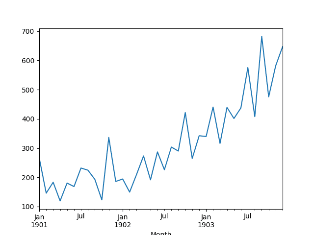
Line Plot of Monthly Shampoo Sales Dataset
Experimental Test Setup
We will split the Shampoo Sales dataset into two parts: a training and a test set.
The first two years of data will be taken for the training dataset and the remaining one year of data will be used for the test set.
For example:
|
1 2 3 |
# split data into train and test X = series.values train, test = X[0:-12], X[-12:] |
Models will be developed using the training dataset and will make predictions on the test dataset.
A rolling forecast scenario will be used, also called walk-forward model validation.
Each time step of the test dataset will be walked one at a time. A model will be used to make a forecast for the time step, then the actual expected value from the test set will be taken and made available to the model for the forecast on the next time step.
For example:
|
1 2 3 4 5 |
# walk-forward validation history = [x for x in train] predictions = list() for i in range(len(test)): # make prediction... |
This mimics a real-world scenario where new Shampoo Sales observations would be available each month and used in the forecasting of the following month.
Finally, all forecasts on the test dataset will be collected and an error score calculated to summarize the skill of the model. The root mean squared error (RMSE) will be used as it punishes large errors and results in a score that is in the same units as the forecast data, namely monthly shampoo sales.
For example:
|
1 2 3 |
from sklearn.metrics import mean_squared_error rmse = sqrt(mean_squared_error(test, predictions)) print('RMSE: %.3f' % rmse) |
Persistence Model Forecast
A good baseline forecast for a time series with a linear increasing trend is a persistence forecast.
The persistence forecast is where the observation from the prior time step (t-1) is used to predict the observation at the current time step (t).
We can implement this by taking the last observation from the training data and history accumulated by walk-forward validation and using that to predict the current time step.
For example:
|
1 2 |
# make prediction yhat = history[-1] |
We will accumulate all predictions in an array so that they can be directly compared to the test dataset.
The complete example of the persistence forecast model on the Shampoo Sales dataset is listed below.
|
1 2 3 4 5 6 7 8 9 10 11 12 13 14 15 16 17 18 19 20 21 22 23 24 25 26 27 |
from pandas import read_csv from pandas import datetime from sklearn.metrics import mean_squared_error from math import sqrt from matplotlib import pyplot # load dataset def parser(x): return datetime.strptime('190'+x, '%Y-%m') series = read_csv('shampoo-sales.csv', header=0, parse_dates=[0], index_col=0, squeeze=True, date_parser=parser) # split data into train and test X = series.values train, test = X[0:-12], X[-12:] # walk-forward validation history = [x for x in train] predictions = list() for i in range(len(test)): # make prediction predictions.append(history[-1]) # observation history.append(test[i]) # report performance rmse = sqrt(mean_squared_error(test, predictions)) print('RMSE: %.3f' % rmse) # line plot of observed vs predicted pyplot.plot(test) pyplot.plot(predictions) pyplot.show() |
Note: Your results may vary given the stochastic nature of the algorithm or evaluation procedure, or differences in numerical precision. Consider running the example a few times and compare the average outcome.
Running the example prints the RMSE of about 136 monthly shampoo sales for the forecasts on the test dataset.
|
1 |
RMSE: 136.761 |
A line plot of the test dataset (blue) compared to the predicted values (orange) is also created showing the persistence model forecast in context.
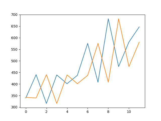
Persistence Forecast of Observed vs Predicted for Shampoo Sales Dataset
For more on the persistence model for time series forecasting, see this post:
Now that we have a baseline of performance on the dataset, we can get started developing an LSTM model for the data.
Need help with LSTMs for Sequence Prediction?
Take my free 7-day email course and discover 6 different LSTM architectures (with code).
Click to sign-up and also get a free PDF Ebook version of the course.
LSTM Data Preparation
Before we can fit an LSTM model to the dataset, we must transform the data.
This section is broken down into three steps:
- Transform the time series into a supervised learning problem
- Transform the time series data so that it is stationary.
- Transform the observations to have a specific scale.
Transform Time Series to Supervised Learning
The LSTM model in Keras assumes that your data is divided into input (X) and output (y) components.
For a time series problem, we can achieve this by using the observation from the last time step (t-1) as the input and the observation at the current time step (t) as the output.
We can achieve this using the shift() function in Pandas that will push all values in a series down by a specified number places. We require a shift of 1 place, which will become the input variables. The time series as it stands will be the output variables.
We can then concatenate these two series together to create a DataFrame ready for supervised learning. The pushed-down series will have a new position at the top with no value. A NaN (not a number) value will be used in this position. We will replace these NaN values with 0 values, which the LSTM model will have to learn as “the start of the series” or “I have no data here,” as a month with zero sales on this dataset has not been observed.
The code below defines a helper function to do this called timeseries_to_supervised(). It takes a NumPy array of the raw time series data and a lag or number of shifted series to create and use as inputs.
|
1 2 3 4 5 6 7 8 |
# frame a sequence as a supervised learning problem def timeseries_to_supervised(data, lag=1): df = DataFrame(data) columns = [df.shift(i) for i in range(1, lag+1)] columns.append(df) df = concat(columns, axis=1) df.fillna(0, inplace=True) return df |
We can test this function with our loaded Shampoo Sales dataset and convert it into a supervised learning problem.
|
1 2 3 4 5 6 7 8 9 10 11 12 13 14 15 16 17 18 19 20 21 22 |
from pandas import read_csv from pandas import datetime from pandas import DataFrame from pandas import concat # frame a sequence as a supervised learning problem def timeseries_to_supervised(data, lag=1): df = DataFrame(data) columns = [df.shift(i) for i in range(1, lag+1)] columns.append(df) df = concat(columns, axis=1) df.fillna(0, inplace=True) return df # load dataset def parser(x): return datetime.strptime('190'+x, '%Y-%m') series = read_csv('shampoo-sales.csv', header=0, parse_dates=[0], index_col=0, squeeze=True, date_parser=parser) # transform to supervised learning X = series.values supervised = timeseries_to_supervised(X, 1) print(supervised.head()) |
Running the example prints the first 5 rows of the new supervised learning problem.
|
1 2 3 4 5 6 |
0 0 0 0.000000 266.000000 1 266.000000 145.899994 2 145.899994 183.100006 3 183.100006 119.300003 4 119.300003 180.300003 |
For more information on transforming a time series problem into a supervised learning problem, see the post:
Transform Time Series to Stationary
The Shampoo Sales dataset is not stationary.
This means that there is a structure in the data that is dependent on the time. Specifically, there is an increasing trend in the data.
Stationary data is easier to model and will very likely result in more skillful forecasts.
The trend can be removed from the observations, then added back to forecasts later to return the prediction to the original scale and calculate a comparable error score.
A standard way to remove a trend is by differencing the data. That is the observation from the previous time step (t-1) is subtracted from the current observation (t). This removes the trend and we are left with a difference series, or the changes to the observations from one time step to the next.
We can achieve this automatically using the diff() function in pandas. Alternatively, we can get finer grained control and write our own function to do this, which is preferred for its flexibility in this case.
Below is a function called difference() that calculates a differenced series. Note that the first observation in the series is skipped as there is no prior observation with which to calculate a differenced value.
|
1 2 3 4 5 6 7 |
# create a differenced series def difference(dataset, interval=1): diff = list() for i in range(interval, len(dataset)): value = dataset[i] - dataset[i - interval] diff.append(value) return Series(diff) |
We also need to invert this process in order to take forecasts made on the differenced series back into their original scale.
The function below, called inverse_difference(), inverts this operation.
|
1 2 3 |
# invert differenced value def inverse_difference(history, yhat, interval=1): return yhat + history[-interval] |
We can test out these functions by differencing the whole series, then returning it to the original scale, as follows:
|
1 2 3 4 5 6 7 8 9 10 11 12 13 14 15 16 17 18 19 20 21 22 23 24 25 26 27 28 29 30 31 |
from pandas import read_csv from pandas import datetime from pandas import Series # create a differenced series def difference(dataset, interval=1): diff = list() for i in range(interval, len(dataset)): value = dataset[i] - dataset[i - interval] diff.append(value) return Series(diff) # invert differenced value def inverse_difference(history, yhat, interval=1): return yhat + history[-interval] # load dataset def parser(x): return datetime.strptime('190'+x, '%Y-%m') series = read_csv('shampoo-sales.csv', header=0, parse_dates=[0], index_col=0, squeeze=True, date_parser=parser) print(series.head()) # transform to be stationary differenced = difference(series, 1) print(differenced.head()) # invert transform inverted = list() for i in range(len(differenced)): value = inverse_difference(series, differenced[i], len(series)-i) inverted.append(value) inverted = Series(inverted) print(inverted.head()) |
Running the example prints the first 5 rows of the loaded data, then the first 5 rows of the differenced series, then finally the first 5 rows with the difference operation inverted.
Note that the first observation in the original dataset was removed from the inverted difference data. Besides that, the last set of data matches the first as expected.
|
1 2 3 4 5 6 7 8 9 10 11 12 13 14 15 16 17 18 19 20 21 |
Month 1901-01-01 266.0 1901-02-01 145.9 1901-03-01 183.1 1901-04-01 119.3 1901-05-01 180.3 Name: Sales, dtype: float64 0 -120.1 1 37.2 2 -63.8 3 61.0 4 -11.8 dtype: float64 0 145.9 1 183.1 2 119.3 3 180.3 4 168.5 dtype: float64 |
For more information on making the time series stationary and differencing, see the posts:
- How to Check if Time Series Data is Stationary with Python
- How to Difference a Time Series Dataset with Python
Transform Time Series to Scale
Like other neural networks, LSTMs expect data to be within the scale of the activation function used by the network.
The default activation function for LSTMs is the hyperbolic tangent (tanh), which outputs values between -1 and 1. This is the preferred range for the time series data.
To make the experiment fair, the scaling coefficients (min and max) values must be calculated on the training dataset and applied to scale the test dataset and any forecasts. This is to avoid contaminating the experiment with knowledge from the test dataset, which might give the model a small edge.
We can transform the dataset to the range [-1, 1] using the MinMaxScaler class. Like other scikit-learn transform classes, it requires data provided in a matrix format with rows and columns. Therefore, we must reshape our NumPy arrays before transforming.
For example:
|
1 2 3 4 5 6 |
# transform scale X = series.values X = X.reshape(len(X), 1) scaler = MinMaxScaler(feature_range=(-1, 1)) scaler = scaler.fit(X) scaled_X = scaler.transform(X) |
Again, we must invert the scale on forecasts to return the values back to the original scale so that the results can be interpreted and a comparable error score can be calculated.
|
1 2 |
# invert transform inverted_X = scaler.inverse_transform(scaled_X) |
Putting all of this together, the example below transforms the scale of the Shampoo Sales data.
|
1 2 3 4 5 6 7 8 9 10 11 12 13 14 15 16 17 18 19 20 21 |
from pandas import read_csv from pandas import datetime from pandas import Series from sklearn.preprocessing import MinMaxScaler # load dataset def parser(x): return datetime.strptime('190'+x, '%Y-%m') series = read_csv('shampoo-sales.csv', header=0, parse_dates=[0], index_col=0, squeeze=True, date_parser=parser) print(series.head()) # transform scale X = series.values X = X.reshape(len(X), 1) scaler = MinMaxScaler(feature_range=(-1, 1)) scaler = scaler.fit(X) scaled_X = scaler.transform(X) scaled_series = Series(scaled_X[:, 0]) print(scaled_series.head()) # invert transform inverted_X = scaler.inverse_transform(scaled_X) inverted_series = Series(inverted_X[:, 0]) print(inverted_series.head()) |
Running the example first prints the first 5 rows of the loaded data, then the first 5 rows of the scaled data, then the first 5 rows with the scale transform inverted, matching the original data.
|
1 2 3 4 5 6 7 8 9 10 11 12 13 14 15 16 17 18 19 20 21 |
Month 1901-01-01 266.0 1901-02-01 145.9 1901-03-01 183.1 1901-04-01 119.3 1901-05-01 180.3 Name: Sales, dtype: float64 0 -0.478585 1 -0.905456 2 -0.773236 3 -1.000000 4 -0.783188 dtype: float64 0 266.0 1 145.9 2 183.1 3 119.3 4 180.3 dtype: float64 |
Now that we know how to prepare data for the LSTM network, we can start developing our model.
LSTM Model Development
The Long Short-Term Memory network (LSTM) is a type of Recurrent Neural Network (RNN).
A benefit of this type of network is that it can learn and remember over long sequences and does not rely on a pre-specified window lagged observation as input.
In Keras, this is referred to as stateful, and involves setting the “stateful” argument to “True” when defining an LSTM layer.
By default, an LSTM layer in Keras maintains state between data within one batch. A batch of data is a fixed-sized number of rows from the training dataset that defines how many patterns to process before updating the weights of the network. State in the LSTM layer between batches is cleared by default, therefore we must make the LSTM stateful. This gives us fine-grained control over when state of the LSTM layer is cleared, by calling the reset_states() function.
The LSTM layer expects input to be in a matrix with the dimensions: [samples, time steps, features].
- Samples: These are independent observations from the domain, typically rows of data.
- Time steps: These are separate time steps of a given variable for a given observation.
- Features: These are separate measures observed at the time of observation.
We have some flexibility in how the Shampoo Sales dataset is framed for the network. We will keep it simple and frame the problem as each time step in the original sequence is one separate sample, with one timestep and one feature.
Given that the training dataset is defined as X inputs and y outputs, it must be reshaped into the Samples/TimeSteps/Features format, for example:
|
1 2 |
X, y = train[:, 0:-1], train[:, -1] X = X.reshape(X.shape[0], 1, X.shape[1]) |
The shape of the input data must be specified in the LSTM layer using the “batch_input_shape” argument as a tuple that specifies the expected number of observations to read each batch, the number of time steps, and the number of features.
The batch size is often much smaller than the total number of samples. It, along with the number of epochs, defines how quickly the network learns the data (how often the weights are updated).
The final import parameter in defining the LSTM layer is the number of neurons, also called the number of memory units or blocks. This is a reasonably simple problem and a number between 1 and 5 should be sufficient.
The line below creates a single LSTM hidden layer that also specifies the expectations of the input layer via the “batch_input_shape” argument.
|
1 |
layer = LSTM(neurons, batch_input_shape=(batch_size, X.shape[1], X.shape[2]), stateful=True) |
The network requires a single neuron in the output layer with a linear activation to predict the number of shampoo sales at the next time step.
Once the network is specified, it must be compiled into an efficient symbolic representation using a backend mathematical library, such as TensorFlow or Theano.
In compiling the network, we must specify a loss function and optimization algorithm. We will use “mean_squared_error” as the loss function as it closely matches RMSE that we will are interested in, and the efficient ADAM optimization algorithm.
Using the Sequential Keras API to define the network, the below snippet creates and compiles the network.
|
1 2 3 4 |
model = Sequential() model.add(LSTM(neurons, batch_input_shape=(batch_size, X.shape[1], X.shape[2]), stateful=True)) model.add(Dense(1)) model.compile(loss='mean_squared_error', optimizer='adam') |
Once compiled, it can be fit to the training data. Because the network is stateful, we must control when the internal state is reset. Therefore, we must manually manage the training process one epoch at a time across the desired number of epochs.
By default, the samples within an epoch are shuffled prior to being exposed to the network. Again, this is undesirable for the LSTM because we want the network to build up state as it learns across the sequence of observations. We can disable the shuffling of samples by setting “shuffle” to “False“.
Also by default, the network reports a lot of debug information about the learning progress and skill of the model at the end of each epoch. We can disable this by setting the “verbose” argument to the level of “0“.
We can then reset the internal state at the end of the training epoch, ready for the next training iteration.
Below is a loop that manually fits the network to the training data.
|
1 2 3 |
for i in range(nb_epoch): model.fit(X, y, epochs=1, batch_size=batch_size, verbose=0, shuffle=False) model.reset_states() |
Putting this all together, we can define a function called fit_lstm() that trains and returns an LSTM model. As arguments, it takes the training dataset in a supervised learning format, a batch size, a number of epochs, and a number of neurons.
|
1 2 3 4 5 6 7 8 9 10 11 |
def fit_lstm(train, batch_size, nb_epoch, neurons): X, y = train[:, 0:-1], train[:, -1] X = X.reshape(X.shape[0], 1, X.shape[1]) model = Sequential() model.add(LSTM(neurons, batch_input_shape=(batch_size, X.shape[1], X.shape[2]), stateful=True)) model.add(Dense(1)) model.compile(loss='mean_squared_error', optimizer='adam') for i in range(nb_epoch): model.fit(X, y, epochs=1, batch_size=batch_size, verbose=0, shuffle=False) model.reset_states() return model |
The batch_size must be set to 1. This is because it must be a factor of the size of the training and test datasets.
The predict() function on the model is also constrained by the batch size; there it must be set to 1 because we are interested in making one-step forecasts on the test data.
We will not tune the network parameters in this tutorial; instead we will use the following configuration, found with a little trial and error:
- Batch Size: 1
- Epochs: 3000
- Neurons: 4
As an extension to this tutorial, you might like to explore different model parameters and see if you can improve performance.
- Update: Consider trying 1500 epochs and 1 neuron, the performance may be better!
Next, we will look at how we can use a fit LSTM model to make a one-step forecast.
LSTM Forecast
Once the LSTM model is fit to the training data, it can be used to make forecasts.
Again, we have some flexibility. We can decide to fit the model once on all of the training data, then predict each new time step one at a time from the test data (we’ll call this the fixed approach), or we can re-fit the model or update the model each time step of the test data as new observations from the test data are made available (we’ll call this the dynamic approach).
In this tutorial, we will go with the fixed approach for its simplicity, although, we would expect the dynamic approach to result in better model skill.
To make a forecast, we can call the predict() function on the model. This requires a 3D NumPy array input as an argument. In this case, it will be an array of one value, the observation at the previous time step.
The predict() function returns an array of predictions, one for each input row provided. Because we are providing a single input, the output will be a 2D NumPy array with one value.
We can capture this behavior in a function named forecast() listed below. Given a fit model, a batch-size used when fitting the model (e.g. 1), and a row from the test data, the function will separate out the input data from the test row, reshape it, and return the prediction as a single floating point value.
|
1 2 3 4 5 |
def forecast(model, batch_size, row): X = row[0:-1] X = X.reshape(1, 1, len(X)) yhat = model.predict(X, batch_size=batch_size) return yhat[0,0] |
During training, the internal state is reset after each epoch. While forecasting, we will not want to reset the internal state between forecasts. In fact, we would like the model to build up state as we forecast each time step in the test dataset.
This raises the question as to what would be a good initial state for the network prior to forecasting the test dataset.
In this tutorial, we will seed the state by making a prediction on all samples in the training dataset. In theory, the internal state should be set up ready to forecast the next time step.
We now have all of the pieces to fit an LSTM Network model for the Shampoo Sales dataset and evaluate its performance.
In the next section, we will put all of these pieces together.
Complete LSTM Example
In this section, we will fit an LSTM to the Shampoo Sales dataset and evaluate the model.
This will involve drawing together all of the elements from the prior sections. There are a lot of them, so let’s review:
- Load the dataset from CSV file.
- Transform the dataset to make it suitable for the LSTM model, including:
- Transforming the data to a supervised learning problem.
- Transforming the data to be stationary.
- Transforming the data so that it has the scale -1 to 1.
- Fitting a stateful LSTM network model to the training data.
- Evaluating the static LSTM model on the test data.
- Report the performance of the forecasts.
Some things to note about the example:
- The scaling and inverse scaling behaviors have been moved to the functions scale() and invert_scale() for brevity.
- The test data is scaled using the fit of the scaler on the training data, as is required to ensure the min/max values of the test data do not influence the model.
- The order of data transforms was adjusted for convenience to first make the data stationary, then a supervised learning problem, then scaled.
- Differencing was performed on the entire dataset prior to splitting into train and test sets for convenience. We could just as easily collect observations during the walk-forward validation and difference them as we go. I decided against it for readability.
The complete example is listed below.
|
1 2 3 4 5 6 7 8 9 10 11 12 13 14 15 16 17 18 19 20 21 22 23 24 25 26 27 28 29 30 31 32 33 34 35 36 37 38 39 40 41 42 43 44 45 46 47 48 49 50 51 52 53 54 55 56 57 58 59 60 61 62 63 64 65 66 67 68 69 70 71 72 73 74 75 76 77 78 79 80 81 82 83 84 85 86 87 88 89 90 91 92 93 94 95 96 97 98 99 100 101 102 103 104 105 106 107 108 109 110 111 112 113 114 115 116 117 118 119 120 121 122 123 124 |
from pandas import DataFrame from pandas import Series from pandas import concat from pandas import read_csv from pandas import datetime from sklearn.metrics import mean_squared_error from sklearn.preprocessing import MinMaxScaler from keras.models import Sequential from keras.layers import Dense from keras.layers import LSTM from math import sqrt from matplotlib import pyplot import numpy # date-time parsing function for loading the dataset def parser(x): return datetime.strptime('190'+x, '%Y-%m') # frame a sequence as a supervised learning problem def timeseries_to_supervised(data, lag=1): df = DataFrame(data) columns = [df.shift(i) for i in range(1, lag+1)] columns.append(df) df = concat(columns, axis=1) df.fillna(0, inplace=True) return df # create a differenced series def difference(dataset, interval=1): diff = list() for i in range(interval, len(dataset)): value = dataset[i] - dataset[i - interval] diff.append(value) return Series(diff) # invert differenced value def inverse_difference(history, yhat, interval=1): return yhat + history[-interval] # scale train and test data to [-1, 1] def scale(train, test): # fit scaler scaler = MinMaxScaler(feature_range=(-1, 1)) scaler = scaler.fit(train) # transform train train = train.reshape(train.shape[0], train.shape[1]) train_scaled = scaler.transform(train) # transform test test = test.reshape(test.shape[0], test.shape[1]) test_scaled = scaler.transform(test) return scaler, train_scaled, test_scaled # inverse scaling for a forecasted value def invert_scale(scaler, X, value): new_row = [x for x in X] + [value] array = numpy.array(new_row) array = array.reshape(1, len(array)) inverted = scaler.inverse_transform(array) return inverted[0, -1] # fit an LSTM network to training data def fit_lstm(train, batch_size, nb_epoch, neurons): X, y = train[:, 0:-1], train[:, -1] X = X.reshape(X.shape[0], 1, X.shape[1]) model = Sequential() model.add(LSTM(neurons, batch_input_shape=(batch_size, X.shape[1], X.shape[2]), stateful=True)) model.add(Dense(1)) model.compile(loss='mean_squared_error', optimizer='adam') for i in range(nb_epoch): model.fit(X, y, epochs=1, batch_size=batch_size, verbose=0, shuffle=False) model.reset_states() return model # make a one-step forecast def forecast_lstm(model, batch_size, X): X = X.reshape(1, 1, len(X)) yhat = model.predict(X, batch_size=batch_size) return yhat[0,0] # load dataset series = read_csv('shampoo-sales.csv', header=0, parse_dates=[0], index_col=0, squeeze=True, date_parser=parser) # transform data to be stationary raw_values = series.values diff_values = difference(raw_values, 1) # transform data to be supervised learning supervised = timeseries_to_supervised(diff_values, 1) supervised_values = supervised.values # split data into train and test-sets train, test = supervised_values[0:-12], supervised_values[-12:] # transform the scale of the data scaler, train_scaled, test_scaled = scale(train, test) # fit the model lstm_model = fit_lstm(train_scaled, 1, 3000, 4) # forecast the entire training dataset to build up state for forecasting train_reshaped = train_scaled[:, 0].reshape(len(train_scaled), 1, 1) lstm_model.predict(train_reshaped, batch_size=1) # walk-forward validation on the test data predictions = list() for i in range(len(test_scaled)): # make one-step forecast X, y = test_scaled[i, 0:-1], test_scaled[i, -1] yhat = forecast_lstm(lstm_model, 1, X) # invert scaling yhat = invert_scale(scaler, X, yhat) # invert differencing yhat = inverse_difference(raw_values, yhat, len(test_scaled)+1-i) # store forecast predictions.append(yhat) expected = raw_values[len(train) + i + 1] print('Month=%d, Predicted=%f, Expected=%f' % (i+1, yhat, expected)) # report performance rmse = sqrt(mean_squared_error(raw_values[-12:], predictions)) print('Test RMSE: %.3f' % rmse) # line plot of observed vs predicted pyplot.plot(raw_values[-12:]) pyplot.plot(predictions) pyplot.show() |
Running the example prints the expected and predicted values for each of the 12 months in the test dataset.
Note: Your results may vary given the stochastic nature of the algorithm or evaluation procedure, or differences in numerical precision. Consider running the example a few times and compare the average outcome.
The example also prints the RMSE of all forecasts. The model shows an RMSE of 71.721 monthly shampoo sales, which is better than the persistence model that achieved an RMSE of 136.761 shampoo sales.
|
1 2 3 4 5 6 7 8 9 10 11 12 13 |
Month=1, Predicted=351.582196, Expected=339.700000 Month=2, Predicted=432.169667, Expected=440.400000 Month=3, Predicted=378.064505, Expected=315.900000 Month=4, Predicted=441.370077, Expected=439.300000 Month=5, Predicted=446.872627, Expected=401.300000 Month=6, Predicted=514.021244, Expected=437.400000 Month=7, Predicted=525.608903, Expected=575.500000 Month=8, Predicted=473.072365, Expected=407.600000 Month=9, Predicted=523.126979, Expected=682.000000 Month=10, Predicted=592.274106, Expected=475.300000 Month=11, Predicted=589.299863, Expected=581.300000 Month=12, Predicted=584.149152, Expected=646.900000 Test RMSE: 71.721 |
A line plot of the test data (blue) vs the predicted values (orange) is also created, providing context for the model skill.
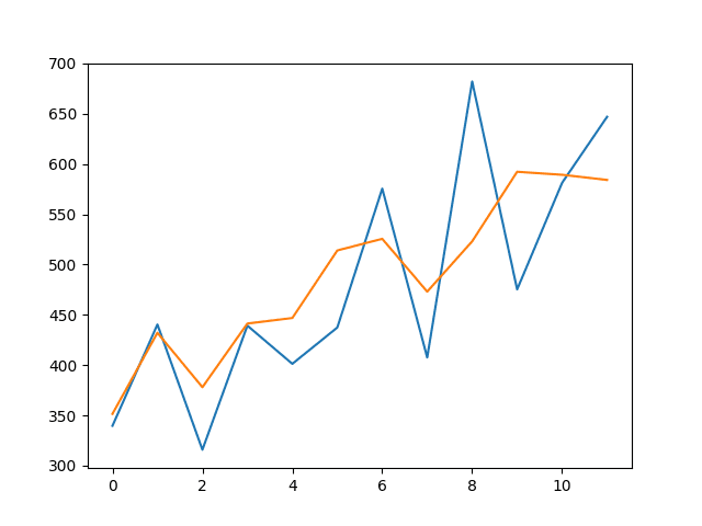
Line Plot of LSTM Forecast vs Expected Values
As an afternote, you can do a quick experiment to build your trust in the test harness and all of the transforms and inverse transforms.
Comment out the line that fits the LSTM model in walk-forward validation:
|
1 |
yhat = forecast_lstm(lstm_model, 1, X) |
And replace it with the following:
|
1 |
yhat = y |
This should produce a model with perfect skill (e.g. a model that predicts the expected outcome as the model output).
The results should look as follows, showing that if the LSTM model could predict the series perfectly, the inverse transforms and error calculation would show it correctly.
|
1 2 3 4 5 6 7 8 9 10 11 12 13 |
Month=1, Predicted=339.700000, Expected=339.700000 Month=2, Predicted=440.400000, Expected=440.400000 Month=3, Predicted=315.900000, Expected=315.900000 Month=4, Predicted=439.300000, Expected=439.300000 Month=5, Predicted=401.300000, Expected=401.300000 Month=6, Predicted=437.400000, Expected=437.400000 Month=7, Predicted=575.500000, Expected=575.500000 Month=8, Predicted=407.600000, Expected=407.600000 Month=9, Predicted=682.000000, Expected=682.000000 Month=10, Predicted=475.300000, Expected=475.300000 Month=11, Predicted=581.300000, Expected=581.300000 Month=12, Predicted=646.900000, Expected=646.900000 Test RMSE: 0.000 |
Develop a Robust Result
A difficulty with neural networks is that they give different results with different starting conditions.
One approach might be to fix the random number seed used by Keras to ensure the results are reproducible. Another approach would be to control for the random initial conditions using a different experimental setup.
We can repeat the experiment from the previous section multiple times, then take the average RMSE as an indication of how well the configuration would be expected to perform on unseen data on average.
This is often called multiple repeats or multiple restarts.
We can wrap the model fitting and walk-forward validation in a loop of fixed number of repeats. Each iteration the RMSE of the run can be recorded. We can then summarize the distribution of RMSE scores.
|
1 2 3 4 5 6 7 8 9 10 11 12 13 14 15 16 17 18 19 20 21 22 23 24 25 |
# repeat experiment repeats = 30 error_scores = list() for r in range(repeats): # fit the model lstm_model = fit_lstm(train_scaled, 1, 3000, 4) # forecast the entire training dataset to build up state for forecasting train_reshaped = train_scaled[:, 0].reshape(len(train_scaled), 1, 1) lstm_model.predict(train_reshaped, batch_size=1) # walk-forward validation on the test data predictions = list() for i in range(len(test_scaled)): # make one-step forecast X, y = test_scaled[i, 0:-1], test_scaled[i, -1] yhat = forecast_lstm(lstm_model, 1, X) # invert scaling yhat = invert_scale(scaler, X, yhat) # invert differencing yhat = inverse_difference(raw_values, yhat, len(test_scaled)+1-i) # store forecast predictions.append(yhat) # report performance rmse = sqrt(mean_squared_error(raw_values[-12:], predictions)) print('%d) Test RMSE: %.3f' % (r+1, rmse)) error_scores.append(rmse) |
The data preparation would be the same as before.
We will use 30 repeats as that is sufficient to provide a good distribution of RMSE scores.
The complete example is listed below.
|
1 2 3 4 5 6 7 8 9 10 11 12 13 14 15 16 17 18 19 20 21 22 23 24 25 26 27 28 29 30 31 32 33 34 35 36 37 38 39 40 41 42 43 44 45 46 47 48 49 50 51 52 53 54 55 56 57 58 59 60 61 62 63 64 65 66 67 68 69 70 71 72 73 74 75 76 77 78 79 80 81 82 83 84 85 86 87 88 89 90 91 92 93 94 95 96 97 98 99 100 101 102 103 104 105 106 107 108 109 110 111 112 113 114 115 116 117 118 119 120 121 122 123 124 125 126 127 128 |
from pandas import DataFrame from pandas import Series from pandas import concat from pandas import read_csv from pandas import datetime from sklearn.metrics import mean_squared_error from sklearn.preprocessing import MinMaxScaler from keras.models import Sequential from keras.layers import Dense from keras.layers import LSTM from math import sqrt from matplotlib import pyplot import numpy # date-time parsing function for loading the dataset def parser(x): return datetime.strptime('190'+x, '%Y-%m') # frame a sequence as a supervised learning problem def timeseries_to_supervised(data, lag=1): df = DataFrame(data) columns = [df.shift(i) for i in range(1, lag+1)] columns.append(df) df = concat(columns, axis=1) df.fillna(0, inplace=True) return df # create a differenced series def difference(dataset, interval=1): diff = list() for i in range(interval, len(dataset)): value = dataset[i] - dataset[i - interval] diff.append(value) return Series(diff) # invert differenced value def inverse_difference(history, yhat, interval=1): return yhat + history[-interval] # scale train and test data to [-1, 1] def scale(train, test): # fit scaler scaler = MinMaxScaler(feature_range=(-1, 1)) scaler = scaler.fit(train) # transform train train = train.reshape(train.shape[0], train.shape[1]) train_scaled = scaler.transform(train) # transform test test = test.reshape(test.shape[0], test.shape[1]) test_scaled = scaler.transform(test) return scaler, train_scaled, test_scaled # inverse scaling for a forecasted value def invert_scale(scaler, X, value): new_row = [x for x in X] + [value] array = numpy.array(new_row) array = array.reshape(1, len(array)) inverted = scaler.inverse_transform(array) return inverted[0, -1] # fit an LSTM network to training data def fit_lstm(train, batch_size, nb_epoch, neurons): X, y = train[:, 0:-1], train[:, -1] X = X.reshape(X.shape[0], 1, X.shape[1]) model = Sequential() model.add(LSTM(neurons, batch_input_shape=(batch_size, X.shape[1], X.shape[2]), stateful=True)) model.add(Dense(1)) model.compile(loss='mean_squared_error', optimizer='adam') for i in range(nb_epoch): model.fit(X, y, epochs=1, batch_size=batch_size, verbose=0, shuffle=False) model.reset_states() return model # make a one-step forecast def forecast_lstm(model, batch_size, X): X = X.reshape(1, 1, len(X)) yhat = model.predict(X, batch_size=batch_size) return yhat[0,0] # load dataset series = read_csv('shampoo-sales.csv', header=0, parse_dates=[0], index_col=0, squeeze=True, date_parser=parser) # transform data to be stationary raw_values = series.values diff_values = difference(raw_values, 1) # transform data to be supervised learning supervised = timeseries_to_supervised(diff_values, 1) supervised_values = supervised.values # split data into train and test-sets train, test = supervised_values[0:-12], supervised_values[-12:] # transform the scale of the data scaler, train_scaled, test_scaled = scale(train, test) # repeat experiment repeats = 30 error_scores = list() for r in range(repeats): # fit the model lstm_model = fit_lstm(train_scaled, 1, 3000, 4) # forecast the entire training dataset to build up state for forecasting train_reshaped = train_scaled[:, 0].reshape(len(train_scaled), 1, 1) lstm_model.predict(train_reshaped, batch_size=1) # walk-forward validation on the test data predictions = list() for i in range(len(test_scaled)): # make one-step forecast X, y = test_scaled[i, 0:-1], test_scaled[i, -1] yhat = forecast_lstm(lstm_model, 1, X) # invert scaling yhat = invert_scale(scaler, X, yhat) # invert differencing yhat = inverse_difference(raw_values, yhat, len(test_scaled)+1-i) # store forecast predictions.append(yhat) # report performance rmse = sqrt(mean_squared_error(raw_values[-12:], predictions)) print('%d) Test RMSE: %.3f' % (r+1, rmse)) error_scores.append(rmse) # summarize results results = DataFrame() results['rmse'] = error_scores print(results.describe()) results.boxplot() pyplot.show() |
Running the example prints the RMSE score each repeat. The end of the run provides summary statistics of the collected RMSE scores.
Note: Your results may vary given the stochastic nature of the algorithm or evaluation procedure, or differences in numerical precision. Consider running the example a few times and compare the average outcome.
We can see that the mean and standard deviation RMSE scores are 138.491905 and 46.313783 monthly shampoo sales respectively.
This is a very useful result as it suggests the result reported above was probably a statistical fluke. The experiment suggests that the model is probably about as good as the persistence model on average (136.761), if not slightly worse.
This indicates that, at the very least, further model tuning is required.
|
1 2 3 4 5 6 7 8 9 10 11 12 13 14 15 16 17 18 19 20 21 22 23 24 25 26 27 28 29 30 31 32 33 34 35 36 37 38 39 |
1) Test RMSE: 136.191 2) Test RMSE: 169.693 3) Test RMSE: 176.553 4) Test RMSE: 198.954 5) Test RMSE: 148.960 6) Test RMSE: 103.744 7) Test RMSE: 164.344 8) Test RMSE: 108.829 9) Test RMSE: 232.282 10) Test RMSE: 110.824 11) Test RMSE: 163.741 12) Test RMSE: 111.535 13) Test RMSE: 118.324 14) Test RMSE: 107.486 15) Test RMSE: 97.719 16) Test RMSE: 87.817 17) Test RMSE: 92.920 18) Test RMSE: 112.528 19) Test RMSE: 131.687 20) Test RMSE: 92.343 21) Test RMSE: 173.249 22) Test RMSE: 182.336 23) Test RMSE: 101.477 24) Test RMSE: 108.171 25) Test RMSE: 135.880 26) Test RMSE: 254.507 27) Test RMSE: 87.198 28) Test RMSE: 122.588 29) Test RMSE: 228.449 30) Test RMSE: 94.427 rmse count 30.000000 mean 138.491905 std 46.313783 min 87.198493 25% 104.679391 50% 120.456233 75% 168.356040 max 254.507272 |
A box and whisker plot is created from the distribution shown below. This captures the middle of the data as well as the extents and outlier results.
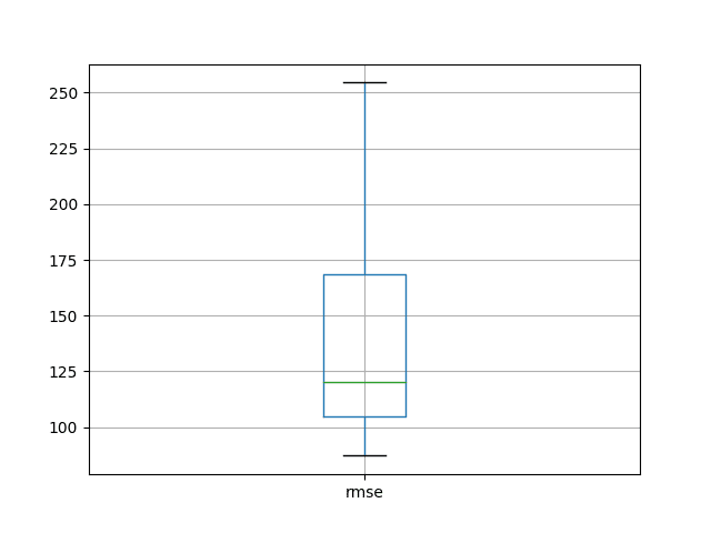
LSTM Repeated Experiment Box and Whisker Plot
This is an experimental setup that could be used to compare one configuration of the LSTM model or set up to another.
Tutorial Extensions
There are many extensions to this tutorial that we may consider.
Perhaps you could explore some of these yourself and post your discoveries in the comments below.
- Multi-Step Forecast. The experimental setup could be changed to predict the next n-time steps rather than the next single time step. This would also permit a larger batch size and faster training. Note that we are basically performing a type of 12 one-step forecast in this tutorial given the model is not updated, although new observations are available and are used as input variables.
- Tune LSTM model. The model was not tuned; instead, the configuration was found with some quick trial and error. I believe much better results could be achieved by tuning at least the number of neurons and number of training epochs. I also think early stopping via a callback might be useful during training.
- Seed State Experiments. It is not clear whether seeding the system prior to forecasting by predicting all of the training data is beneficial. It seems like a good idea in theory, but this needs to be demonstrated. Also, perhaps other methods of seeding the model prior to forecasting would be beneficial.
- Update Model. The model could be updated in each time step of the walk-forward validation. Experiments are needed to determine if it would be better to refit the model from scratch or update the weights with a few more training epochs including the new sample.
- Input Time Steps. The LSTM input supports multiple time steps for a sample. Experiments are needed to see if including lag observations as time steps provides any benefit.
- Input Lag Features. Lag observations may be included as input features. Experiments are needed to see if including lag features provide any benefit, not unlike an AR(k) linear model.
- Input Error Series. An error series may be constructed (forecast error from a persistence model) and used as an additional input feature, not unlike an MA(k) linear model. Experiments are needed to see if this provides any benefit.
- Learn Non-Stationary. The LSTM network may be able to learn the trend in the data and make reasonable predictions. Experiments are needed to see if temporal dependent structures, like trends and seasonality, left in data can be learned and effectively predicted by LSTMs.
- Contrast Stateless. Stateful LSTMs were used in this tutorial. The results should be compared with stateless LSTM configurations.
- Statistical Significance. The multiple repeats experimental protocol can be extended further to include statistical significance tests to demonstrate whether the difference between populations of RMSE results with different configurations are statistically significant.
Summary
In this tutorial, you discovered how to develop an LSTM model for time series forecasting.
Specifically, you learned:
- How to prepare time series data for developing an LSTM model.
- How to develop an LSTM model for time series forecasting.
- How to evaluate an LSTM model using a robust test harness.
Can you get a better result?
Share your findings in the comments below.
Develop Deep Learning models for Time Series Today!

Develop Your Own Forecasting models in Minutes
...with just a few lines of python code
Discover how in my new Ebook:
Deep Learning for Time Series Forecasting
It provides self-study tutorials on topics like:
CNNs, LSTMs,
Multivariate Forecasting, Multi-Step Forecasting and much more...
Finally Bring Deep Learning to your Time Series Forecasting Projects
Skip the Academics. Just Results.


I’ve been working on multi-step-ahead forecast after reading your ebook and following one step ahead tutorials. But still struggling getting nothing. It seems that seq2seq model is used, but I want to configure simple lstm for multi step ahead prediction. Can you help me in getting basic idea to do this?
Yes, I have some seq2seq examples scheduled to come out on the blog soon.
This is all fine and well but how do you do a true step ahead forecast BEYOND the dataset? Every blog I see just shows comparison graphs of actual and predicted. How do you use this model to simply look ahead x number of periods past the data, with no graphs? Thanks!
Hi Shawn,
Perhaps the following may help clear up some confusion with a slightly different approach.
https://www.youtube.com/watch?v=tepxdcepTbY&t=24s
Hi Jason,
Thank you for this blog. I am working on multi-step-ahead forecast using recursive prediction technique and I have some difficulty. Blog on this particular topic would be really helpful.
Also, is it possible to somehow implement recursive technique in ARIMA?.
Absolutely, you can take the predictions as history and re-fit the ARIMA.
Thanks for the suggestion, it would make a good blog post.
I am wondering if I have predictions (not good prediction) and refitting without validating with the test set, wouldn’t it give false prediction again?
It may, design an experiment to test the approach.
Hi Jason,
Thanks for this blog. Can you please share an example of multi-step-ahead forecast using recursive prediction technique using LSTM.
Thanks,
Shifu
Thanks for the suggestion.
I have an example of a direct model for multi-step forecasting here:
https://machinelearningmastery.com/multi-step-time-series-forecasting-long-short-term-memory-networks-python/
Hi Jason,
LSTM remember sequences but is there a way to encode calendar effects in the network so that it remembers or learns events that occur at different intervals within the sequence and each cycles? A concrete example would be a time series that exhibits specific events that repeat themselves on specific times in the year, example first Monday of every month and/or last day of every month. I am thinking whether we can label this data in advance to help the LSTM predict these events better?
Hello Peter,
You might want to check out the X-11 method to separate trend, seasonal, and random change to your sequence. Then apply an algorithm to each part.
You can look at the following article :
Study of the Long-term Performance Prediction Methods Using the Spacecraft Telemetry Data
from Hongzeng Fang
(Sorry but I can’t find a free dl page anymore ..).
Thanks for the tip.
Hey Jason, in the case of taking the last observation in the dataset in order to predict the next future timestep (for which we don’t have current values for), does the model use only that 1 observation to predict the next??? Or because it’s an LSTM , does it use both the memory from all the preceding observations during training + the last observation in order to predict the next timestep?
If it’s the latter – it would make more sense to me. Otherwise I can’t see the sense in using nothing but 1 observation to predict one ahead and guarantee any type of accuracy.
The way the model is defined, an input sequence is provided in order to predict one time step.
You can define the mapping any way you wish for your problem though.
Hi Jason,
Nice post. Is there any tutorial available on multivariate time series forecasting problem?
I got two sets of data: traffic flow data and weather data. I am thinking to predict the traffic flow using these two data sets.
I’d like to learn if I get weather condition involved what will happen for my model.
Could you kindly give me some advice?
Thank you.
I do not have a multivariate regression example, but I hope to post one soon.
Great. Thank you in advance.
That would be awesome, indeed
Hi Jason. It is really a nice example of using LSTM. I’m working on it.
I also have the same question, are you going to give an example on multivariate time series forecasting? I’m struggling on it.
I have an example here:
https://machinelearningmastery.com/multivariate-time-series-forecasting-lstms-keras/
You did a great job. This is very detailed ! Bravo 😉
I’m glad you found it useful Gabriel.
Great tutorial,
How do we get a prediction on a currently not existing point in the future?
yhat = model.predict(X)
I mean without a y.
Error measurements are cool, but I also want to make a prediction for a next step.
That’s my main intention to read this tutorial.
Since there are other tutorials out there, lacking the same issue, it would be great to have a complete example, with a real live ouput/result/value.
I’m aware of the fact that every problem should have its own solution/model, but with a real result (or a comprehensible way to it), the code would be more practical/reusable- especially for python-ml beginners trying to predict some values in the future.
Fit your model on the entire training dataset then predict the next time step as:
Hi Jason, thanks for your tutorial. But can you specify how to fit the model on the entire training set and do the prediction for future point? Thanks.
That is just a little too much hand holding Donna. What are you having trouble with exactly?
Hi, Jsson:
yhat = model.predict(X):X means current values? and yhad means predict value?
Yes, X is the input required to make one or more predictions and yhat are the predictions.
Hi, Jason, just got one question related to prediction. Since in your example, you own did prediction one test data,(known), where you have the row data to inverse the difference. What about the prediction for future unknown data, how can we do the difference inversion ?
Yes, inverting the difference for a prediction only requires the last known observation.
Thank you Jason,
I’m new to Python (mainly coding other languages) and just beginning to understand the code- thanks to your outstanding detailed descriptions.
In the last weeks I tried out two other tutorials and failed exactly at this point (making a first own test-appliance with a result).
A) Could you please suggest a location/row number in the code in one of the examples for that line?
B) Is there a magic trick available to avoid the date conversion and work with real dates in own data sets?
In the moment I would have to transform my data to that date format of the used raw data.
I’m afraid to break the code logic.
But I also try to research every crucial part of the code separately for example here:
https://docs.scipy.org/doc/numpy/reference/arrays.indexing.html
My current Python skills are on the level of this tutorial
https://www.youtube.com/watch?v=N4mEzFDjqtA .
Hi Hans,
What do you mean by “first own test-appliance with a result”. I don’t follow.
Do you mean make a prediction? If so you can make a prediction by fitting the model no all of your data and calling model.predict(X).
Pandas is really flexible when it comes to loading date data. A good approach for you might be to specify your own date parsing function to use when loading your data. See this post for an example that does this:
https://machinelearningmastery.com/stateful-stateless-lstm-time-series-forecasting-python/
Worth to mention (latest Windows-Info 4.2017):
There is an issue with Keras/Anaconda on Windows.
To run the last example above on Win, we have to manually reinstall Keras.
Further informations can be found here:
https://github.com/llSourcell/How-to-Predict-Stock-Prices-Easily-Demo/issues/3#issuecomment-288981625
…otherwise it throws compiling errors.
Does this tutorial work for you?
https://machinelearningmastery.com/setup-python-environment-machine-learning-deep-learning-anaconda/
I already saw this tutorial written by you.
On Windows (not a Mac) it’s a slightly different story to build such an environment, even with Anaconda.
It begins with the fact that there is no Tensorflow with a version <= 3 for Windows and ends with the Keras-hint.
We needed several days to discuss it on Github and find the right setup in the context of another RNN-script (see the link).
I use virtual conda-environments and your scripts are running on windows if the keras-hint is implemented.
Before I had the same issue with some of your scripts then with the discussed one on Github (compile error).
Update, what I mean:
I guess one could trigger “forecast_lstm(model, batch_size, X)” or “yhat = model.predict(X)” from the end of the last two example scripts.
But how to do that in regard to the trained model?
“Month=13, Predicted=???”
Do I have to define a new “fictional” X? And if so how?
You must load the new input data for which a prediction is required as X and use your already fit model to make the prediction by calling the predict() function.
I’m eager to help, but perhaps I don’t understand the difficulty exactly?
Hi again Jason! brilliant tutorial once again,
I believe many people is asking about the model.predict() because it’s not really working as expected.
First problem is that doing:
yhat = model.predict(X)
with the code example previously given, returns:
NameError: name ‘model’ is not defined
As I understand, this is because the model is created under the name “lstm_model” instead of model, so using:
yhat = lstm_model.predict(X)
works, but returns:
ValueError: Error when checking : expected lstm_1_input to have 3 dimensions, but got array with shape (1, 1)
So, personally, what I have done, is using the “forecast_lstm” function, this way:
yhat = forecast_lstm(lstm_model, 1, X)
print(yhat)
0.28453988
Which actually returns a value.
Now the next problem is that the X, is nothing else than the last X of the example, as I never redefine it.
I found that the amount of functions and filters applied to the training data is quite big, hence I need to replicate them to make the shape match.
This is my original training data.
series = read_sql_query(seleccion, conn, parse_dates=[‘creacion’], index_col=[‘creacion’])
print(series)
sys.exit()
menores
creacion
2018-06-17 03:56:11 0.0
2018-06-17 03:54:03 2.0
2018-06-17 03:52:11 4.0
2018-06-17 03:50:05 6.0
2018-06-17 03:48:17 4.0
2018-06-17 03:46:04 4.0
2018-06-17 03:44:01 4.0
2018-06-17 03:43:05 1.0
2018-06-17 03:40:12 2.0
2018-06-17 03:38:12 0.0
2018-06-17 03:36:21 4.0
2018-06-17 03:34:32 4.0
2018-06-17 03:32:05 3.0
2018-06-17 03:30:01 2.0
2018-06-17 03:28:23 1.0
2018-06-17 03:26:17 3.0
2018-06-17 03:24:04 0.0
2018-06-17 03:22:34 4.0
2018-06-17 03:20:04 2.0
2018-06-17 03:18:18 2.0
2018-06-17 03:16:00 3.0
2018-06-17 03:14:06 6.0
2018-06-17 03:12:06 4.0
2018-06-17 03:10:04 2.0
2018-06-17 03:08:02 0.0
2018-06-17 03:06:02 4.0
2018-06-17 03:04:02 4.0
2018-06-17 03:02:10 3.0
2018-06-17 03:00:22 4.0
2018-06-17 02:59:13 3.0
… …
[7161 rows x 1 columns]
Then, this process is applied to “series”:
# transform data to be stationary
raw_values = series.values
diff_values = difference(raw_values, 1)
# transform data to be supervised learning
supervised = timeseries_to_supervised(diff_values, 1)
supervised_values = supervised.values
if you print “supervised_values” at that point, the original data has been transformed to:
[[0 array([4.])]
[array([4.]) array([-3.])]
[array([-3.]) array([1.])]
…
[array([2.]) array([4.])]
[array([4.]) array([-3.])]
[array([-3.]) array([-1.])]]
which is clearly less and more condensed information…
Therefore, if I try to apply
yhat = forecast_lstm(lstm_model, 1, X)
after the new data has been loaded:
predecir = read_sql_query(seleccion, conn, parse_dates=[‘creacion’], index_col=[‘creacion’])
#limpiamos la cache
conn.commit()
print(predecir)
print(X)
yhat = forecast_lstm(lstm_model, 1, X)
#ynew = ynew[0]
print(yhat)
I get the following error:
AttributeError: ‘DataFrame’ object has no attribute ‘reshape’
————
So kinda lost in how to actually apply the same structure to the new data before being able to make the new prediction!
I’ll paste the source my code in case someone needs it:
https://codepen.io/anon/pen/xzPVxE
You’ll see that I’m loading the data directly from MySQL, and also, splitting the training and test data with a different approach from a previous example given in the blog!
I’m not sure either about how to make the next prediction!
Thanks a lot for this blog once again… I wouldn’t be even trying this if it wasn’t for your help and explanations!!!
My best wishes,
Chris
Thanks for sharing.
I have solved this the same way as suggested in this Stack Overflow post: https://stackoverflow.com/questions/42240376/dataframe-object-has-no-attribute-reshape
I am no more directly invoking the reshape method in the pandas training and test DataFrames, but indirectly through their values:
train = train.values.reshape(train.shape[0], train.shape[1])
test = test.values.reshape(test.shape[0], test.shape[1])
I’m happy to hear that.
Hello Jason,
I knew I shouldn’t mention the date conversion part :-). Meanwhile I managed it with “return datetime.strptime(x, ‘%Y-%m-%d’)”
I have all of your example script parts in separate python file version. So I can test out modifications for specific requirements.
python basic_data_loading.py

python persistence_forecast_model.py

python transform_time_series_to_supervised.py

python transform_time_series_to_statonary_remove_trends.py

python transform_scales.py

python complete_example.py
Own data loading is solved. That was a relatively easy task.
Since the transforming and performance measurement parts are running (I guess they will do even with integer data)
I now have to build a part lets call it:
“python predict_one_value.py”
Of course I have to load my own data that’s clear.
The question is where to trigger the function
yhat = model.predict(X)
in the context of one of your example-scripts and finally say:
print(yhat). That’s all.
I guess a short example snippet could solve the problem.
Could you provide an example- It would help a lot?
Currently I also don’t understand the role of X completely.
In the context of “datetime.strptime” it seems to be a date only, If I print it out.
So if I would have training data of:
– 01.12.1977
– 02.12.1977
– 03.12.1977
I would guess I could say something like “yhat = model.predict(“1977-12-04″)”.
The question is where and when in which code context.
Thank you.
Update:
Currently I use the the code from “complete example” (“without robust result”).
If I comment out from line 106 to line 127 and then at the end of the script say:
# report one value in the future

test = datetime.strptime('2017-04-15', '%Y-%m-%d')

yhat = model.predict(test)

print(yhat)
I get the error message ‘model is not defined’. So trying…
# report one value in the future

test = datetime.strptime('2017-04-15', '%Y-%m-%d')

yhat = lstm_model.predict(test)

print(yhat)
…throws the error “Data should be a Numby array”.
I guess maybe I could also append a new date to the raw data (without a y),
but I’m not sure If this would be right.
The best way to get this running would be an example snipped in context.
This post will give you a clearer idea of how to use neural nets in Keras including making predictions:
https://machinelearningmastery.com/5-step-life-cycle-neural-network-models-keras/
Yes, input data to making a prediction must be a 2D numpy array. It will not be date data, it will be past obs in the case of time series forecasting.
Thank you,
I will read it ;-).
I have read the tutorial and tried out the pima indians diabetes example.
I guess I got it and understand the 5 steps (mostly).
Unfortunately this does not answer my question. Or do I miss something?
In my problem I have only one input like in the tutorial on this site.
When you say:
“yhat = model.predict(X)”
would give a forecast for a next step.
What about a step which is not in the training data nor in the test data?
I have a SVM model which proves and predicts based on my raw data (realized in another environment).
Lets say I have 100 items training data, 10 items test data.
It will printout 10 predictions and additionally corresponding performance data.
The last printed prediction is for a future step which lies in the future.
How would this be archived in your example?
Do I have to shift something?
To make predictions beyond your dataset, you must feed in the last few observations from your dataset as input (X) to predict what happens next (y).
This post might clear up your thinking on X and y:
https://machinelearningmastery.com/time-series-forecasting-supervised-learning/
>To make predictions beyond your dataset, you must feed in the last few observations from your dataset as input (X) to >predict what happens next (y).
Is there an example available where this is done?
Yes, the “LSTM Forecast” section of this very post.
Assuming that “X = row[0:-1]” is an observation,
how do we sample/collect the last few observations, to make a forecast.?
It depends on your model, if your model expects the last one observation as input, then reframe that value as a 2d array and provide it as X to model.predict(X).
If your model requires the last two lag obs as inputs, retrieve them, define them as a one row, two column matrix and provide them to model.predict().
And so on. I hope that helps.
HI Jason,
Even i started with machine learning and have similar kind of doubt so in one step forecasting we can only get one time step future observation correct ? and to get the prediction i have provided last input observation and then the value obtained from model.predict(X) has to be again scaled and inversed correct ?
PFB the code:
X = test_scaled[3,-1:] (my last observation)
yhat = forecast_lstm(lstm_model, 1, X)
yhat = invert_scale(scaler, X, yhat)
yhat = inverse_difference(raw_values, yhat, 1)
print(yhat)
Can you please guide me if i am going in a right way ?
Yes, one step forecasting involves predicting the next time step.
You can make multi-step forecasts, learn more in this post:
https://machinelearningmastery.com/multi-step-time-series-forecasting/
Yes, to make use of the prediction you will need to invert any data transforms performed such as scaling and differencing.
Thank you Jason ..
Hi Jason,
Being said that, i have another clarification , so when i forecast the next time step using this model , using the below code:
X = test_scaled[3,-1:] (my last observation)
yhat = forecast_lstm(lstm_model, 1, X)
yhat = invert_scale(scaler, X, yhat)
yhat = inverse_difference(raw_values, yhat, 1)
print(yhat)
in the above code, let yhat be the prediction of future time step, can i use the result of yhat and use the same model to predict one more step ahead in the future ? is this what we call as the recursive multistep forecast ?
Yes. This is recursive.
Hi Jason,
Can i use the below code and use the recursive multistep forecast
for eg :
yhat value can be used as an input to the same model again to get the next future step and so on ?
X = test_scaled[3,-1:] (my last observation)
yhat = forecast_lstm(lstm_model, 1, X)
yhat = invert_scale(scaler, X, yhat)
yhat = inverse_difference(raw_values, yhat, 1)
print(yhat)
Hi Jason,
In predictive analytics using this ML technique, how many future steps should we able to predict , is there any ideal forecasting range in future for eg if i have a data for the last 10 days or so , and i want to forecast the future , the less the future time steps are set, the better the result as the error will be minimum right. Can i use the same code for predicting time series data in production for network traffic for future 3 days ? requirement given for me was to predict the network bandwidth for the next entire week given the data for past 1 year.
Your comments and suggestions always welcome 🙂
Regards,
Arun
It depends on the problem and the model.
Generally, the further in the future you want to predict, the worse the performance of the model.
Hello,
can we normalize the RMSE-value(s)?
And if so how?
Normalize the skill score?
Yes, but you will need to know the largest possible error.
I’m feeding your example with values ranged from 1 to 70.
There is no increasing trend in my raw data.
When it comes to predictions the script predicts values above 70.
Regarding to the other tutorial (5 Step Life-Cycle) I think it has to do with the compile part (model.compile).
But I’m not sure. Could you provide a comprehensible hint in regard of the example script on this site?
Hi Jason,
assuming you had multiple features (you can add one feature to the shampoo dataset) and wanted to use multiple timesteps, what would the dataset look like that I put into the model? Is it a 3 dimensional array, where the features are lists of values and each observation is a list of these features and the label(s) (which is also a list of values)?
Good question, it would be a 3D array with the dimensions [samples, timesteps, features].
Right now the model gives only one step forecast. What if I wanted to create a model which gives forecast for next 60 months.
I will have a post on this see, until then see this post:
https://machinelearningmastery.com/multi-step-time-series-forecasting/
Hi Jason, I have a question.
raw_values = series.values
diff_values = difference(raw_values, 1)
print(len(raw_values)) 36
print(len(diff_values)) 35
So, after difference we lose the first value?
Correct.
Dear Jason,
Thank you very much for this extremely useful and interesting post.
I may be missing something, but I think there is one omission: By differencing you loose the trend including its start and end level. Later on you try restore the trend again, but in your code it seems you fail to restore the end level. IMO the end level of the current observations should be added to all the predictions.
Thanks again!
What do you mean by the end level? Sorry I don’t follow, perhaps you could restate your comment?
Great tutorial!
Quick question: On the scaling section of the tutorial you say that
“To make the experiment fair, the scaling coefficients (min and max) values must be calculated on the training dataset and applied to scale the test dataset and any forecasts. This is to avoid contaminating the experiment with knowledge from the test dataset, which might give the model a small edge.”
However, if the max of your sample is on the test dataset the scaling with parameters from the training set will yield a number outside the [-1,1] range. How can one deal with that?
Thanks!
Correct.
One good approach is to estimate the expected min and max values that are possible for the domain and use these to scale.
If even then you see values out of range, you can clamp them to the bounds 0/1.
Dear Jason,
To be more precise: you should add the difference between the start level and the end level of the train set. This is because the current code effectively replicates the train set. By this I means that it starts at the same level as the train set. However, it should start at the end level of the train set.
Kind regards,
Guido
I will try to restate my comment:
Currently the predictions (of your test set) start at the same level as the observations (in your train set). Therefore, there is a shift between the last observed value (in your train set) and the first predicted value (of your test set). The size of this shift is equal to: start level of the observations minus end level of the observations (in your train set). You should correct for this shift by adding it to the predicted values.
Isn’t this made moot by making the data stationary?
Hello,
1. can you please explain me the below 2 lines in detail.
model.add(LSTM(neurons, batch_input_shape=(batch_size, X.shape[1], X.shape[2]), stateful=True))
model.add(Dense(1))
2. I want to know the layer architecture. What are the number of neurons in hidden layer?
3. If I want to add one more hidden layer, how the syntax looks like?
4. What could be the reason for test rmse is less than train rmse?
The line defines the input layer and the first LSTM hidden layer with “neurons” number of memory units.
You can stack LSTMs, the first hidden layer must return sequences (return_sequence=True) and you can add a second LSTM layer. I have an example here:
https://machinelearningmastery.com/time-series-prediction-lstm-recurrent-neural-networks-python-keras/
Better performance on the test data than the training data may be a sign of an unstable/underfit model.
Hallo Jason, thank you for this post! I bought the first version of your book and I have seen you have in the meantime deeper analysed this topic. Very good! 🙂 Something have I yet not clear.
“Samples: These are independent observations from the domain, typically rows of data.
Time steps: These are separate time steps of a given variable for a given observation.”
I could understand the case where the time step parameter is 1 as in your book and in this example but I can’t figure out why and how it could be grater than 1…
My hypothesys, sure wrong 🙂
Perhaps when a timestep is made of n observations one could give the value n to it…but then I would expect when one in the model writes (pag. 192):
“model.add(LSTM(4, input_shape=(1, look_back)))”
the LSTM would use (look_back * timesteps) rows for every step to predict the next row…
I cannot also understand why you say ‘of a given variable’…a row is normally built by the values of many variables, isn’t it?
Could you give me an example with timesteps > 1? Thank you!
Hi Fabio,
The structure of the input to the LSTM is [samples, timesteps, features]
If you have multiple observations at one time step, then these are represented as features.
Does that help?
Hello Jason,
unfortunately If don’t have a concrete example I cannot fully understand…The examples in your posts and your book are clear to me but they are always on timesteps=1…if I’m not wrong. For example how could be adapted the szenario described in this post in order to manage a timesteps>1?
Thank you very much!
PS. In the meantime I bought also your book on time series 🙂
See this post on multi-step forecasting:
https://machinelearningmastery.com/multi-step-time-series-forecasting/
Thanks Jason for the wonderful tutorial!
I am using your tutorial to apply LSTM network on some syslog/network log data.
I have syslog data(a specific event) for each day for last 1 year and so I am using LSTM network for time series analysis.
As I understand from your tutorial.
1. A batch of data is a fixed-sized number of rows from the training dataset that defines how many patterns to process before updating the weights of the network. Based on the batch_size the Model takes random samples from the data for the analysis. For time series this is not desirable, hence the batch_size should always be 1.
2. By default, the samples within an epoch are shuffled prior to being exposed to the network. This is undesirable for the LSTM because we want the network to build up state as it learns across the sequence of observations. We can disable the shuffling of samples by setting “shuffle” to “False“.
Scenario1 –
Using above two rules/guidelines – I ran several trials with different number of neurons, epoch size and different layers and got better results from the baseline model(persistence model).
Scenario2-
Without using above guidelines/rules – I ran several trials with different number of neurons, epoch size and different layers and got even better results than Scenario 1.
Query – Setting shuffle to True and Batch_size values to 1 for time series. Is this a rule or a guideline?
It seems logical reading your tutorial that the data for time series should not be shuffled as we do not want to change the sequence of data, but for my data the results are better if I let the data be shuffled.
At the end what I think, what matters is how I get better predictions with my runs.
I think I should try and put away “theory” over concrete evidence, such as metrics, elbows, RMSEs,etc.
Kindly enlighten.
Random samples are not taken, LSTMs require sequence data to be ordered – they learn order dependence.
The “shuffle” argument must be set to “False” on sequence prediction problems if sequence data is spread across samples.
Dear Jason,
I have two hours time series data which consists of 120 observations, using LSTM RNN how can I predict next 30 observation while putting all my data to training section.
We normally split the original data set in two data set ( test dataset and validation dataset) for checking our model performance. I would like to see that my model is only taking help from training dataset to produce an output that does match with validation data set. What I understand from several of your blogs that we are forecasting single value and using that single forecasting along with the help of validation dataset we are forecasting rest of values. I believe I getting lost there? How it is going to work when have only past and current data ( suppose no validation data) and we want to predict the next half an hour.
For example, suppose I have data of a product price from 12 to 1:30pm which consists of 90 observations and using these past 90 observations can we forecast the price of that product during 1:31 to 2:00pm(otherwise next 30 observations) .
Would you please help me to solve the confusion that I have? By the way I am going through your books time series forecasting with Python and deep learning with Python.
You can make a multi-step model with an LSTM by using it directly (predict n timesteps in a one shot manner) or recursively (use the same model again and again and use predictions as inputs for subsequent predictions).
More on multi-step forecasting here:
https://machinelearningmastery.com/multi-step-time-series-forecasting/
Does that help?
Thanks for quick replay
Looks like you sleep very less as you have provided feedback on early morning from your site.
Thanks for being so kind to your students. May god bless you.
By the way do you have any blog or example for second option that you have provided me(use the same model again and again and use predictions as inputs for subsequent predictions). Obviously I would like to see that I am not using any data from validation dataset or not getting any feedback from validation data. Model should only from past and current data along with current predictions. I hope you got this confused student.
Thanking you
Sorry, I don’t have an example of using the model recursively. I believe you could adapt the above example.
would you please give me some hint where I have to change the code to make the model recursive as I am not very good at coding.
Predictions would be used as history (input) to make predictions on the subsequent time steps.
Thanks Jason for the wonderful tutorial!
A little problem here:
def invert_scale(scaler, X, value):

	new_row = [x for x in X] + [yhat]

        ...
Does it should be
def invert_scale(scaler, X, value):

	new_row = [x for x in X] + [value]

        ...
Thanks Max.
I’m getting the following error when running the first block of code you provide.
TypeError: strptime() argument 1 must be str, not numpy.ndarray
It seems like this a problem with how Python 3.6 handles byte strings.
I have only tested the code on Python 2.7 and Python 3.5, perhaps try one of those?
Otherwise, you may need to adapt the example for your specific platform, if an API change is indeed the cause of your issue.
The issue was with the text in footer ‘Sales of shampoo over a three year period’.
Either delete the footer OR
Change the line:
series = read_csv(‘shampoo-sales.csv’, header=0, parse_dates=[0], index_col=0, squeeze=True, date_parser=parser)
to:
series = read_csv(‘shampoo-sales.csv’, header=0, parse_dates=[0], index_col=0, squeeze=True, date_parser=parser, skipfooter=2)
I think that error is caused by the line of descriptive text at the bottom of the shampoo sales data file. If you see this comment at the bottom of the data file, remove it:
Sales of shampoo over a three year period
The data file also has the dates enclosed in double quotes. A couple of times that bit me too. The date_parser callback is a little fickle.
Hello, Your examples are great, thanks.
I have a question:
1- What do we do with the array of predicted values when we use lstm_model.predict() with train data in the example? It seems like they are not being used. Is it important for the net?
Thanks Logan.
What do you mean exactly? Is there a specific section and line of code you are referring to in the tutorial?
Yes, line 101 lstm_model.predict(train_reshaped, batch_size=1) on section Complete LSTM Example.
By the way, I have another question: When the differentiation is applied to the entire dataset, isn’t it giving information about the test dataset to the model?
Thanks. You’ve been helping me a lot.
In this case yes, but in practice, we can apply the same method to the test data using data from training step-wise without cheating.
Hi Jason, I’m also having the same question as Logan mentioned above. Line 101
lstm_model.predict(train_reshaped, batch_size=1)
do we need this line.
I comment this line, and I see no difference. Could you explain a bit more why we need this line ?
Thank you for the great tutor.
Best, Long
It is supposed to seed the state on the training data.
If it does not add value, remove it.
Hi Jason,
Thanks so much for this helpful tutorial. Could you clarify which of all the parameters need to be updated to change the lag value? I haven’t been able to get it to work.
Thanks!
Great question.
Change the parameters to the timeseries_to_supervised() function
I had to change the limits of the range() function to get the loop to work for lag values > 1.
def timeseries_to_supervised(data, lag=1):
df = DataFrame(data)
columns = [df.shift(i) for i in range(lag, 0, -1)]
columns.append(df)
df = concat(columns, axis=1)
df.fillna(0, inplace=True)
return df
Nice!
Hi Jason,
I have been following you for quite sometime now. Another great example for time series. I remember trying out sliding window approach in one of the earlier blogs. I am still waiting for you to write up a blog on involving external features(it can be as simple as (is_weekday =0/1 is_weekend=0/1) and see how its implemented.
can you point out where we can add the above external variables in the above example and the format please for these features please. I will try it out. being new to python its very confusing with these reshapes and pre -format required for LSTM s
#aspring data scientist, student
You can add them as separate features.
I am working on an example at the moment. I hope to post it when it gives good results.
Hi Jason, nice example! I have your similar problem, but I don’t know how resolve. I have a two different class to predict, in different files. I have to training my neural network with this different files. The problem is that each file has different number of samples, and I have to use the same LSTM for each file.How I can generalize the number of input for each LSTM??
This is my problem:
https://drive.google.com/file/d/0B5hOtU0Xa45RUDJJWHVyeHVNQWM/view?usp=sharing
Maybe this post will help you better understand your prediction problem and frame it as supervised learning:
https://machinelearningmastery.com/how-to-define-your-machine-learning-problem/
Thanks for the answere, I have understand which is my problem. It depends from the training, because I have a lot of file for training, and when I insert a new file and remake the fit, the previusly information are forgotten. Do you have some examples for train the LSTM with more file? And where each one has the supervisioned learning, apply to time-series and predict information? Thank you!
Yes, this example shows how to update an existing model with more data:
https://machinelearningmastery.com/update-lstm-networks-training-time-series-forecasting/
Dear Jason:
You did a great job!!
Thank you for sharing the great post with us.
I’m a beginner to machine learning, these days i am busy on doing a project to predict the movement of ship on the sea.
I found this post is very usefull and easy to understand.
I have one question that:
if the number of neurons is the past steps used to predict next step?
Thank you for answer in advance.
Best wishes
I’m not sure what you mean.
The number of neurons defines the size/complexity of the model. The model is used to make predictions.
Perhaps you could reframe your question?
Hi,
Congrats for the blog, and thanks! It helped me a lot.
I have one question related to the data transformation. I understand the step to make that one input is the last output, so the LSTM can learn and save that info. But I have a different case (classification) and I don’t know how could I apply this.
In my case my inputs are images (frames from a video) what have a temporal dependency, and my outputs are numbers (0,1 or 2). First I want to pass the images through a CNN network and then take the features and those would be my LSTM input. In that case, it is necessary to process the data as you have done here? I thought the LSTM would save that info by itself, but now I’m not so sure.
Thank you in advance.
I don’t have an example of working with video data.
Generally, the principles would be the same. As a classification problem, you would need to change the output layer to use one of the log loss activation functions. The input would be from a CNN or similar, e.g. [cnn]->[lstm]->[dense].
Let me know how you go.
Hey did you ever get this working I have a similar problem I would like to address and would value your input!!
In your ARIMA tutorial you also use the shampoo data set, but measure accuracy by MSE. Making the change to RMSE:
rmse = sqrt(mean_squared_error(test, predictions))

print('Test RMSE: %.3f' % rmse)
I get:
> Test RMSE: 83.417
Can we conclude that ARIMA is far better than an LSTM for this problem so far in our research?
No, these are demonstrations. Both algorithms would require tuning to present the best version of themselves (“steel man” vs “straw man”) for model selection.
We are writing the timeseries_to_supervised function to accept a lag:
def timeseries_to_supervised(data, lag=1):
Is this feature to essentially the Window Method + reshaping described in your July 21, 2016 tutorial?
But we don’t seem to use that parameter, always “timeseries_to_supervised(diff_values, 1)”
Using lag values up to around 50 (on the airline data) and changing predict() like so:
# forecast the entire training dataset to build up state for forecasting

train_reshaped = train_scaled[:, 0:look_back].reshape(len(train_scaled), 1, look_back)

# train_reshaped = train_scaled[:, 0].reshape(len(train_scaled), 1, 1)

lstm_model.predict(train_reshaped, batch_size=1)
seems to make good predictions with very low RMSE on test.
Am I possibly breaking the model now so it’s cheating somehow?
look_back = 60

epochs = 15
Month=1, Predicted=321.813110, Expected=315.000000
Month=2, Predicted=310.719757, Expected=301.000000
Month=3, Predicted=363.746643, Expected=356.000000
...
Month=46, Predicted=458.424683, Expected=461.000000
Month=47, Predicted=418.427124, Expected=390.000000
Month=48, Predicted=412.831085, Expected=432.000000
Test RMSE: 18.078
for test harness
yhat = y

Test RMSE: 0.000
It seems there is contamination of training data in the test forecast in the sense that forecast_lstm(model, batch_size, X) is being given X observations, each with 60 historical past observations that overlap into training data. But so what, right? That’s history that training saw, and as it moves into the test data it adds history only seen in the test set. But that’s how real life observations work it seems: You always have all of the past to look at.
Finally, you say, “In this tutorial, we will go with the fixed approach for its simplicity, although, we would expect the dynamic approach to result in better model skill.” For a small dataset like we have, a large lag seems as if it gives us a semi-dynamic approach in some ways?
Solid model with a seemingly good RMSE?
Full code: http://tinyurl.com/y74ypvde
Prediction v. Actual Plot: http://tinyurl.com/y9ouajdm
On the Shampoo dataset:
look_back = 18 (lag)
epochs = 30
Test RMSE: 110.594
Prediction v. Actual Plot: http://tinyurl.com/ycoy6aes
Very sharp!
Nice.
Hmmm, I believe by dynamic I was referring to updating the model with new data.
If you have the resources, I would recommend exploring whether updating the model as new obs come in effects model skill. I expect it will. I have an example here:
https://machinelearningmastery.com/update-lstm-networks-training-time-series-forecasting/
Hi Jason,
You’re doing a great job helping people to learn how to apply machine learning. One week ago, I didn’t know anything about time series, but now I’m able to play a little bit with it. Thanks you!
Regarding this post, I’ve a doubt. When we say
‘To make the experiment fair, the scaling coefficients (min and max) values must be calculated on the training dataset and applied to scale the test dataset and any forecasts. This is to avoid contaminating the experiment with knowledge from the test dataset, which might give the model a small edge.’
shouldn’t we do
scaler = scaler.fit(X[:-12])
instead of
scaler = scaler.fit(X) ?
If we use X we are using data from the test set, no?
Thanks for your attention and keep up with the good work!
Correct. Ideally, we would use domain knowledge to estimate the expected min/max of values that could ever be observed.
Hello Jason,
After using the robust code (last one) I got theses results
1) Test RMSE: 180.438
2) Test RMSE: 110.352
3) Test RMSE: 119.655
4) Test RMSE: 170.720
5) Test RMSE: 211.877
6) Test RMSE: 101.453
7) Test RMSE: 105.532
8) Test RMSE: 149.351
9) Test RMSE: 88.118
10) Test RMSE: 138.013
11) Test RMSE: 265.045
12) Test RMSE: 135.861
13) Test RMSE: 167.766 … (rest is omitted, it was taking too long).
Being a beginner in machine learning and using your tutorial to learn about it could you tell me if theses results are normal (being so different from what you have) while everything before was ok. If theses are not, could you tell my what could be the reason of such difference?
Thank you for your attention and please do continue making tutorial like that, it’s really helpful!
Hi Eric, see this post to better understand the stochastic nature of neural network algorithms:
https://machinelearningmastery.com/randomness-in-machine-learning/
See this post for more details on how to develop a robust estimate of model skill:
https://machinelearningmastery.com/evaluate-skill-deep-learning-models/
See this post on how to fix the random number seed:
https://machinelearningmastery.com/reproducible-results-neural-networks-keras/
I see, thank you very much for the links and solutions!
You’re welcome.
After reading the links what I understood was:
– It’s pretty hard (impossible) to always get the same result due to a lot of randomness that can come from a lot of thing.
– Only by repeating the operation a lot (like you did on last example, with 30 example (but doing it like 100 would give a better idea?)) can help you to determine how much result can be different and find a range of “acceptable one”?
– Seeding the random number generator can help.
So to continue my project I thought about seed the random number generator like you explained. Like here, repeat the process 30 time (since I have a server I can let it do it overnight and go for 100) and determine the average and decide of a range.
Does it seem ok to begin with?
Am I lacking something?
Thank you for your attention and for the help you provide to everyone.
See this post on how to estimate the number of repeats:
https://machinelearningmastery.com/estimate-number-experiment-repeats-stochastic-machine-learning-algorithms/
I would not recommend fixing the random number seed for experimental work. Your results will misleading.
Hi Jason,
Thank you so much for the tutorial.
I have few doubts though.
1. I am working on a problem where the autocorrelation plot of the detrended data show me that the value at time t is significantly correlated to around past 100 values in the series. Is it ideal to take the batch size of 100 to model the series?
2. You mentioned that less than 5 memory units is sufficient for this example. Can you please give me some idea on how to choose the number of memory units for a particular problem like the above? On what other factors does this number depend on?
Kindly clarify.
Thanks
Try passing in 100-200 time steps and see how you go.
Systematically test a suite of different memory units to see what works best.
Thank you Jason.
You’re welcome.
Hey Jason! Thanks a lot for this tutorial, it really helped.
I used this tutorial as is for predicting the cost of an item which is of the the range of a dollar and few cents.
My dataset has 262 rows, i.e 0 to 261.
When I run the model, the graph captures even the most intricate trends beautifully, BUT there seems to be a lag of 1 time step in the predicted data.
The predicted values of this month almost exactly matches the expected value of the previous month. And this trend is followed throughout.
The indexing is the only thing I’ve changed,
to
train, test = supervised_values[0:200], supervised_values[200:]
rmse = sqrt(mean_squared_error(raw_values[200:], predictions))
pyplot.plot(raw_values[200:])
are the only lines of code I’ve really changed
Consider starting with a simpler linear model:
https://machinelearningmastery.com/start-here/#timeseries
I do not believe LSTMs are the best or first choice for autoregression models:
https://machinelearningmastery.com/suitability-long-short-term-memory-networks-time-series-forecasting/
I think I’m facing the same issue. Were you able to solve the issue?
Hi, Jason
Doesn’t LSTM have a squashing gate at input? With outputs in between (-1, 1)? Then why do we need to prepare the input data to be between (-1, 1) if the first input gate will do this for us?
Am I missing something?
Yes, you can rescale input to [0,1]
Considering
unseenPredict = lstm_model.predict(X)
…how do we structure X to get a one step forward prediction of unseen data?
Or can we change some offsets in script “Complete LSTM Example” to get the same effect, and if so how?
Hi Jason,
Thanks for the excellent tutorial. I tried to modify the above code to include multiple timesteps and multiple lags in the model. I run give these parameters as input and paralleling run the script for different configurations to select the most accurate model. What do you think of the modifications I have done to the following functions? I am especially concerned about the time_steps included in the model, is that correct?
def timeseries_to_supervised(data, lag=1, time_steps=0):
df = DataFrame(data)
columns = [df.shift(i) for i in range(1, lag+1)]
#considers the number of time_steps, t, involved and
#add next t x columns next to each x columnn
#question?? if time_steps = 3, does that mean y should start from y_4 and
#we trim the last 3 values from the dataset?
if time_steps > 0 :
columns_df = concat(columns,axis=1)
#note that I have multipled i by -1 to perform left shift rather than right shift
timestep_columns = [columns_df.shift(i*-1) for i in range(1, time_steps+1)]
timestep_columns_df =concat(timestep_columns, axis=1)
columns.append(timestep_columns_df)
columns.append(df)
df = concat(columns, axis=1)
df.fillna(0, inplace=True)
return df
def fit_lstm(train, batch_size, nb_epoch, neurons, lag, time_steps):
X, y = train[:, 0:-1], train[:, -1]
X = X.reshape(X.shape[0], time_steps+1, lag)
model = Sequential()
model.add(LSTM(neurons, batch_input_shape=(batch_size, X.shape[1] , X.shape[2]), stateful=True, return_sequences=True))
model.add(LSTM(neurons, stateful=True))
model.add(Dense(1))
model.compile(loss=’mean_squared_error’ optimizer=’adam’)
model.summary()
for i in range(nb_epoch):
model.fit(X, y, epochs=1, batch_size=batch_size, verbose=1, shuffle=False)
model.reset_states()
return model
def forecast_lstm(model, batch_size, X, lag,time_steps):
X = X.reshape(1,time_steps+1,lag)
pad = np.zeros(shape=(batch_size-1, time_steps+1, lag))
padded = np.vstack((X, pad))
yhat = model.predict(padded, batch_size=batch_size)
return yhat[0,0]
Great work!
I want to extend this idea to several features x the lag values for each x time observations. Does it seem reasonable to give MinMaxScaler that 3D object? How does the y truth fit in what I give MinMaxScaler, since it’s only 2D?
No, I would recommend scaling each series separately.
Above you seem to scale y along with X. But with multiple features, the rest of which are not just a time-shifted copy of y, I assume we could fit y_train by itself before transforming y_train and y_val? Then that’s actually the only scaler object we need to save for later inversion?
I would recommend scaling each series before any shifting of the series to make it a supervised learning problem.
I hope that answers your question, please shout if I misunderstood.
I think the words “each series separately” threw me. I assume we can still scale all incoming values (all X’s and the time series that will later become y and shifted, one of the X’s) using a single scaler object. Then we create the lag values from scaled values. Finally, that single scaler object is used to invert y predictions. I have that right?
Each series being a different “feature” or “column” or “time series” or whatever we call it.
The coefficients (min/max or mean/stdev) used in the scaling of each series will need to be kept to reverse the operation on predictions and apply the operation to input data later. You can save the coefficients or the objects that wrap them.
Jason, great tutorial, thank you!
A question: why do you loop through epochs instead of just setting an appropriate number of epochs within fit() function? Would’t it give the same result and be neater?
So that I can manually manage the resetting of the internal state of the network.
Ah, I see, it has to do with “stateful” definition being different in keras, it’s well explained here: http://philipperemy.github.io/keras-stateful-lstm/
Hi, DR jason
thank you very much for this tutorial.
I want to have multiple time steps , but i don’t know how to modify function “timeseries_to_supervised()”.
I found another post of you talking about this , but you use function “create_dataset()”
i modify this function as follow:
def create_dataset(dataset, look_back=1):
dataset = np.insert(dataset,[0]*look_back,0)
dataX, dataY = [], []
for i in range(len(dataset)-look_back):
a = dataset[i:(i+look_back)]
dataX.append(a)
dataY.append(dataset[i + look_back])
dataY=numpy.array(dataY)
dataY = np.reshape(dataY,(dataY.shape[0],1))
dataset = np.concatenate((dataX,dataY),axis=1)
return dataset
please, check my modification , is it right OR what?
See this post:
https://machinelearningmastery.com/convert-time-series-supervised-learning-problem-python/
Hi Jason,
Sorry if it seem stupid but there is a part that I don’t understand.
To predict you use: “yhat = model.predict(X, batch_size=batch_size)”
But as we see X is :
train, test = supervised_values[0:-12], supervised_values[-12:]
scaler, train_scaled, test_scaled = scale(train, test)
yhat = forecast_lstm(lstm_model, 1, X)
So X is the 12 value (after being passed in the scale function) that we want to predict. Why are we using them since in normal case we wouldn’t know theirs values.
Once again really thank you for your tutorial, really helped me in my training on machine learning.
In the general case, you can pass in whatever you like in order to make a prediction.
For example, if your model was defined by taking 6 days of values and predicting the next day and you want to predict tomorrow, pass in the values for today and 5 days prior.
Does that help?
I think it does help me. In my case I have values for each minute and I have to predict the next week (so more or less 10K of prediction).
I have data from the last year so there isn’t any problem with my training, just wondered what I should do at the prediction part (so I can just instead of feeding it test_scaled send him my training set again?)
Thank you for your help and quick reply!
Yes, if your model is setup to predict given some fixed set of lags, you must provide those lags to predict beyond the end of the dataset. These may be part of your training dataset.
I don’t think it’s in my training dataset, for this part I’m pretty much doing it like you (the lag appearing when turning a sequence to a supervised learning problem). I’m pretty much feeding my model like you do. The problem for me being to know what to feed it when calling the predict command. Sending it “train_scaled” was a bad idea (got poor result, predicting huge value when it should predict low and predicting low instead of predicting high). I’m working on it but every hint is accepted. Once again thank you and sorry for being a bit slow at learning/understanding.
The argument to the predict() function is the same as the argument to the fit() function.
The data must be scaled the same and have the same shape, although the number of samples may vary, e.g. you may have just one sample.
Obviously, you don’t need to make predictions for the training data, so the data passed to predict will be the input required to make the prediction you require. This really depends on the framing of your problem/model.
Does that help?
Thank your for your quick reply! I think I’m understanding it better but I have some part I have trouble to understand.
The input is X right?
If I follow your tutorial on input/output (https://machinelearningmastery.com/time-series-forecasting-supervised-learning/) and I take my case as an example (the database register the value each 3 minute and we want to predict the next value (so to begin for example it would be 12:24:00)):
Date,congestion
2016-07-08 12:12:00,92
2016-07-08 12:15:00,80
2016-07-08 12:18:00,92
2016-07-08 12:21:00,86
This is (part of) my training data, when turning it into supervised training data (and shifting) I get:
X, y
?, 92
92, 80
80, 92
92, 86
86, ?
The problem is that I don’t know X for predicting, I only know the X I use for my training (train_scaled) and the one used to compare my results (test_scaled).
What is the input I should feed it? I can’t feed it my test_scaled since in real situation I would have no idea of what it would be.
Sorry if my question seem stupid and thank you for taking time to explain it.
It depends how you have framed your model.
If the input (X) is the observation at t-1 to predict t, then you input the last observation to predict the next time step.
It is, each of my input X is the observation at t-1 (pretty similar to the shampoo case used in the tutorial).
Thank you for your answer, you answered my question, I shouldn’t have any problem now!
Thanks for the tutorial too, they really helped me!
Glad to hear that.
Just to be sure that I didn’t made any mistake in my reasoning, if I take my example from before:
X, y
?, 92 / T-3
92, 80 / T-2
80, 92 / T-1
92, 86 / T
86, ? / T+1
to predict the next step (T+1) I have to use “yhat = model.predict(X, , batch_size=batch_size)” where X is 86 (after scaling/reshaping). Right?
Then I’ll get the value predicted for T+1 (that I have to send to invert_scale and difference to get a readable value).
If I want to predict farther then I continue (sending the scaled/reshaped value predicted at T+1 to get T+2 and then until I predict as far as wanted).
Thanks for your time and answers!
Correct.
Thank you Jason with your help I managed to predict value of each minute of the next week. I had 2 question though:
First: I removed the code for testing sets (since I wouldn’t have it in reality), the only thing I have are the testing set in the excel file (the last 10000 lines)
When using this code (to train):
# transform data to be stationary
raw_values = data.values
diff_values = difference(raw_values, 1)
# transform data to be supervised learning
supervised = timeseries_to_supervised(diff_values, 1)
supervised_values = supervised.values
# split data into train and test-sets
train = supervised_values[:-10000]
# transform the scale of the data
scaler, train_scaled = scale(train)
and this one (to predict):
# forecast the entire training dataset to build up state for forecasting
train_reshaped = train_scaled[:, 0].reshape(len(train_scaled), 1, 1)
lstm_model.predict(train_reshaped)
# walk-forward validation on the test data
predictions = list()
predictionFeeder = list() #Used to feed the model with the value of T-1
X, y = train_scaled[0, 0:-1], train_scaled[0, -1]
predictionFeeder.append(X) #Give the last value of training
for i in range(0, 10000):
# make one-step forecast
yhat = forecast_lstm2(lstm_model, predictionFeeder[i])
predictionFeeder.append(yhat)
# invert scaling
yhat2 = invert_scale(scaler, testa[i + 1], yhat)
yhat3 = inverse_difference(raw_values, yhat2, 10000 + 1 – i)
predictions.append(yhat3)
and train a model (25 epoch) then predict the results I get result that are way too good (RMSE of 2 or less and prediction that have less than 5% of error).
Being used of thing going wrong for no reasons I decide to remove the testing data from the excel (even though it shouldn’t change anything since I’m not using them (I’ve even set the variable to None at first)). Then when I do that the prediction is way less good and have some lag (though, if you remove the lag you still have a good results, just way less better than before).
Why is that?
My 2nd question is about lag, we can see on the prediction that while the shape of both chart (prediction and reality) look alike the prediction is raising/lowering before the reality, do you have any idea to fix it? Do you think changing the lag or timestep would help?
Once again thank you for your help, I don’t think I would have achieved this much without your tutorials.
Sorry, I cannot debug your code for you.
Perhaps you are accidentally fitting the model on the training and test data then evaluating it on the test (e.g. on data it has seen before).
I would encourage you to evaluate different lag values to see what works best for your problem.
Don’t worry, I wouldn’t ask you to debug.
Maybe, I don’t know, I did remove the variable to be sure to never have affected the testing set and using it but since I’m human I may have made errors.
So changing lag would help me for theses gap between reality and prediction raise. Thank you I’ll do that.
Thanks for your answer!
Can I buy your books physically(not Ebook)?Thanks
Sorry, now I have read that is not possible. Thanks anyway. Your explanations and tutorials are amazing. Congratulations!
Thanks Josep.
Hi,
Thanks for very good tutorial. I have one question/doubt.
in the following part of the code:
# invert differencing
yhat = inverse_difference(raw_values, yhat, len(test_scaled)+1-i)
should not we relay on predicted value instead of already known raw_values? In your example for validation we always refer to the test value(known) while calling inverse difference. But in reality we will have only the predicted values(used as X), and of course known starting point(t=0). Or I missed something?
my proposal:
# invert differencing – (starting from 2nd loop cycle (1st woul be the starting point (raw_values[-1]) )
yhat = inverse_difference(predictions, yhat, 1)
Thanks in advance
Pawel
We could, but in this case the known observations are available and not in the future and it is reasonable to use them for the rescaling (inverting).
Hi, Thanks for explanation, got it now. Cause I train the model used e.g. MAY data (15 seconds samples) and then used that model to predict whole JUNE data. Afterwards I compared predicted data VS data that I got from JUNE, and I have to say that model does not work, after few prediction there is huge “off sync”,
In the validation phase as described in your case I got RMSE 0.11 so not bad, but in reality when you use predicted value(t-1) to predict next (t) value there is a problem.
Do you know how to improve the model? should I use multiple step forecats, or lag features, input time steps?
Thanks a lot.
Pawel
I would recommend braining storming, then try everything you can think of.
I have a good list here:
https://machinelearningmastery.com/improve-deep-learning-performance/
Also, compare results to well-tuned MLPs with a window.
Hey Jason, I am not following one point in your post. You wanted to train a state-full LSTM but reset_states() is executed after every epoch. That means, the states from previous batch are not used in the current batch. How does it make the network state-full?
Thanks
State is maintained between the samples within one epoch.
Hi Jason,
thanks for the great tutorial. I have one question. Wouldn’t it be better to use a callback for resetting the states? This would enable you to also use for example an EarlyStopping Monitor while training, here is what I changed:
class resetStates(Callback):
def on_epoch_end(self, epoch, logs=None):
self.model.reset_states()
model.fit(X, y, epochs=nb_epoch, batch_size=batch_size, verbose=1, shuffle=False, callbacks=[resetStates(),EarlyStopping(monitor=’loss’, patience=5, verbose=1, mode=’min’)])
Yes, that is a cleaner implementation for those problems that need to reset state at the end of each epoch.
Hello, can we extend this for anomaly detection techniques ?
Perhaps, I have not used LSTMs for anomaly detection, I cannot give you good advice.
Perhaps you would frame it as sequence classification?
Hi Jason,
In the persistence model plot there is a one time interval lag. When making single step predictions, is it possible to overcome this issue? What is causing this to happen? It seems like the model places a huge weight on time interval x[t-1].
Here is an example of the dataset I am analyzing:
iteration: 969
Month=970, Predicted=-7.344685, Expected=280.000000
iteration: 970
Month=971, Predicted=73.259611, Expected=212.000000
iteration: 971
Month=972, Predicted=137.053028, Expected=0.000000
Expected should be 280 and 212 (high magnitudes), and the model captures this more or less with 73 and 137, but this is one time interval behind.
Thanks!
LSTMs are not great at autoregression problems and often converge to a persistence type model.
Ok thanks. What model would be a good alternative to capture this issue? I ran into the same problem with ARIMA. It could just be a difficult dataset to predict.
I recommend starting with a well-tuned MLP + Window and see if anything can do better.
Hi Jason,
Thanks to you I managed to get a working LSTM network who seem to have a good accuracy (and so a low RMSE)
But I’ve got a problem, do you know what could be the cause of extreme delay between reality values and predictions (my predictions have the same shape as the reality but increase/decrease way before reality)?
Best regards and please continue what you are doing, it’s really useful.
Hi Eric, it might be a bug in the way you are evaluating the model.
It might be the case, I had to make some changes to the prediction system to use the last predicted value, I may have missed something at this moment. (Also I have to use Tflearn instead of Tensorflow but it shouldn’t be a problem since Tflearn is a more transparent way to use tensorflow).
Thank you for your answer!
Hang in there Eric!
Thank you!
Well.. I have a gap of 151 (reference to pokemon?).
Just to try I removed theses 151 values from my training set, I now have no gap of values (and frankly, the accuracy seem good for a 15 epoch training). I know that this is no way a fix but make me wonder where did I fail..
Could it be that while my training set is on 400K of value my prediction start 151 value before the end (so predicting the value for 399849) of the training set (which is strange since the information from training tell me that I’m training on the 400K of data).
It would mean that my machine is trying to predict some point of time used for training.
Or it would mean that the 151 last data weren’t used at all for training (I tried to reduce the number of data but it’s the same problem).
The algorithm is trained sample by sample, batch by batch, epoch by epoch. The last sample is what is key.
Thanks for the reply.
When I think about it my prediction is in advance compared to the reality.
So my model start his prediction not where I finished my training but after (which is strange since my training end where my testing begin and that each input are a value (and each line correspond to a minute like the the line of shampoo data sets correspond to month)).
I must have made a mistake somewhere.
Thanks for you answer I think I’m on something!
Hang in there!
One thing I don’t understand in these models is, how can I predict future.
Say, I have trained my model and let’s say we’re living August 8, 2017. Now model.predict() seems to require some test samples to predict anything, in this case values from test_scaled. So what do I give it when I want to get a prediction for August 9, 2017, which we don’t know yet? So I want to know yhat(t+1). Can I ask the model to give me forecasts for the next 5 days?
I may be wrong but in my case I trained my model on the data I had (let’s say one year, until August 8, 2017) and to predict the value T you send the value T-1 (so in this case the value of August 8 2017), you’ll get the value of August 9.
Then if you want August 10 (T+1) you send the value of August 9 (T). But this code here show a one step forecast implementation. Maybe if you want to predict more you should look for multi step forecasting? I’m think there is some example of it on this website.
Jason would give you a better answer I think.
Nice one Eric!
Yes, I’ll add, if the model was trained to predict one day from the prior day as input, then when finalized, the model will need the observation from the prior day in order to predict the next day.
It all comes down to how you frame the prediction problem that determines what the inputs you need.
If you would like to predict one day, the model needs to be trained to predict one day.
You have to decide what the model will take as input in order to make that prediction, e.g. the last month or year of data. This is how the model is trained.
Then, when it’s trained, you can use it to predict future values using perhaps the last few values from the training data. You can use a model trained to predict one day to predict may days in a recursive manner where predictions become inputs for subsequent predictions. More about that here:
https://machinelearningmastery.com/multi-step-time-series-forecasting/
You can also make multi-step forecasts directly, here is an example:
https://machinelearningmastery.com/multi-step-time-series-forecasting-long-short-term-memory-networks-python/
Does that make things clearer?
Thanks Eric and Jason. That’s exactly how I’ve done it, but it seems to me, that the prediction that I get is not one timestep forward (T+1), but it’s a prediction of T, which doesn’t make sense. I’m using close price of a stock as my data. I’ll have to check again, if it’s really is making a prediction for the future, as you insist. and I will check the Jason’s links.
Anyways, thanks Jason for the excellent tutorials! 🙂
Here’s a sample of the close prices:
2017-05-30 5.660
2017-05-31 5.645
2017-06-01 5.795
2017-06-02 5.830
As a matter of fact, it seems to me that the predicted values lags one time step behind from expected ones.
Day=1, Predicted=5.705567, Expected=5.660000
Day=1, Predicted=5.671651, Expected=5.645000
Day=1, Predicted=5.657278, Expected=5.795000
Day=1, Predicted=5.805318, Expected=5.830000
Here I’m going forwarding one day at a time and as you see the predicted ones are closer to what was expected one day before than. And anyway,
Let’s examine the second line:
Day=1, Predicted=5.671651, Expected=5.645000
The expected price (which is the actual price on 2017-05-31) is what I give the model on 2017-05-31 after the trading day is closed. What I expect the model to predict is closer to 5.79 than 5.67 (which is closer to the actual price the day before!). See the problem? Have I missed something? I haven’t changed anything in the framework except the data.
That is a persistence model and the algorithm will converge to that (e.g. predict the input as the output) if it cannot do better.
Perhaps explore tuning the algorithm.
Also, I believe security prices are a random walk and persistence is the best we can do anyway:
https://machinelearningmastery.com/gentle-introduction-random-walk-times-series-forecasting-python/
Please do some tutorials RNN, NN with more categorical values in the dataset? please, I could not find many resources using the categorical values.
Thanks
I have a few tutorials on the blog – for example, text data input or output are categorical variables.
What are you looking for exactly?
is it possible to write the code RNN Regression ,what is the activation function i need to give for regression RNN,how it is difference from classification to regression?
Yes. The output would be ‘linear’ for regression.
Hi Dr. Brownlee,
I am trying to understand this code. I am a beginner working with time-series and LSTM.
My questions about your code:
1. What does “transform data to be stationary” mean?
2. Why do you create diff? What does it mean?
3. If the raw_values are 36 data, why diff has only 35?
I appreciate your response in advance,
Maria
Never mind, I already understand. 🙂
Glad to hear it.
Consider using the blog search.
More about stationary data here:
https://machinelearningmastery.com/time-series-data-stationary-python/
More about differencing here:
https://machinelearningmastery.com/remove-trends-seasonality-difference-transform-python/
I hope that helps.
Thanks, for the awesome blogs,
But, I have a doubt, for time series forecasting, classical methods like autoregression and ARIMA, or this machine learning approach using LSTM RNN model, which is the better approach? Both are good on their own, So, what should be our first choice while forecasting any dataset? How should we choose between them?
It depends on your problem. Try a few methods and see what works best.
I recommend starting with linear methods like ARIMA, then try some ML methods like trees and such, then an MLP, then perhaps an RNN.
When I changed train/test ration to 0.8/0.2 in LSTM code, it took half an hour to predict, and with another data that contains around 4000 records, it’s taking hours(i still couldn’t get result, i don’t know how long it’ll take). Can you please suggest me how I change settings for very long sequences. Thanks
I have some ideas here:
https://machinelearningmastery.com/handle-long-sequences-long-short-term-memory-recurrent-neural-networks/
Hi Jason, for long sequence like 4000 records, can you please help me to understand the changes from code point of view as per your current example, the above link is for classification and i am looking for sequence prediction problem.
You must split your sequence into subsequences, for example, see this post for ideas:
https://machinelearningmastery.com/truncated-backpropagation-through-time-in-keras/
Thank you Jason, can you please help us to understand with a complete code example ? The above link just have an idea but not a code implementation, I want to understand from code point of view.
Regards,
Arun
Is the evaluation method in this post really “walk-forward”? I’ve read your post about time-series backtest. Walk-forward corresponds to cross validation for not time series data. In both, we make many models to learn, so these methods are not suitable for deep learning, including LSTM, the theme of this post.
Yes, we are using walk-forward validation here.
Walk-forward validation is required for sequence prediction like time series forecasting.
See this post for more about the method and when to use it:
https://machinelearningmastery.com/backtest-machine-learning-models-time-series-forecasting/
Thank you for your reply. Sorry, that’s not what I mean it. I’ve read the post you pasted above, in which you split data into train/test 2820 times and build 2820 models. But, in this LSTM post, you split data and build a LSTM network only once, so I suggest the test in this article is not walk forward. ordered(not shuffle) hold-out test?
sorry, please delete this comment
Above, the model is evaluated 30 times.
Within the evaluation of one model, we use walk forward validation and samples are not shuffled.
I recommend re-reading the tutorial and code above.
Thank you for your reply! Oh, repeat=30! Sorry, I misunderstood. But I think in the back-test article, the size of train data changes, while in this LSTM article, the size of train data is fixed, right? Sorry for so many questions.
Thanks for your work, it is seriously awesome.
I wanted to see the chart comparing training loss vs validation loss per epoch, see the chart here: https://ibb.co/kqcnBk. As you mentioned in your other post:
“From the plot of loss, we can see that the model has comparable performance on both train and validation datasets (labeled test). If these parallel plots start to depart consistently, it might be a sign to stop training at an earlier epoch.”
However, in this case, the test loss never really gets lower and both lines are not parallel at all. for this problem, and in general, does that mean that no meaningful test-set pattern is learned from the training, as seems to be corroborated by the RMSE being close on average to the persistent/dummy method?
Is this the end of the road? Have NN’s failed in their tasks? If not, where to go next?
The main thing I changed in the code was the end of the fit_lstm function:
for i in range(nb_epoch):
e=model.fit(X, y, epochs=10, batch_size=batch_size, verbose=0,validation_split=0.33, shuffle=False)
model.reset_states()
return model, e
Thanks Gauthier.
It may mean that the model under provisioned for the problem.
OK… So in this case would you suggest to include more neurons for example, or try another ML algorithm?
Both would be a safe bet.
Hi, @Gauthier, may i know how you editted ur code to get the loss function?
Json,
Thanks for your blogs and tutorials. Being a research scholar, when I was in dilemma how to learn ML, your tutorials gave me an excellent start to carry out my work in Machine Learning and Deep Learning.
I tried to work with the example in this page, But, I couldnt download the shampoo_sales dataset from datamarket.com. Could you please put the link to the datasets in the blog? If any procedure to download, please let me know.
Thanks, I’m glad to hear that.
Here is the full dataset:
Hi Jason,
I am getting NAN on the 12 month:::
Month=1, Predicted=440.400000, Expected=440.400000
Month=2, Predicted=315.900000, Expected=315.900000
Month=3, Predicted=439.300000, Expected=439.300000
Month=4, Predicted=401.300000, Expected=401.300000
Month=5, Predicted=437.400000, Expected=437.400000
Month=6, Predicted=575.500000, Expected=575.500000
Month=7, Predicted=407.600000, Expected=407.600000
Month=8, Predicted=682.000000, Expected=682.000000
Month=9, Predicted=475.300000, Expected=475.300000
Month=10, Predicted=581.300000, Expected=581.300000
Month=11, Predicted=646.900000, Expected=646.900000
Month=12, Predicted=646.900000, Expected=nan
from the code below:
predictions = list()
for i in range(len(test_scaled)):
# make one-step forecast
X, y = test_scaled[i, 0:-1], test_scaled[i, -1]
#yhat = forecast_lstm(lstm_model, 1, X)
yhat=y
# invert scaling
yhat = invert_scale(scaler, X, yhat)
# invert differencing
yhat = inverse_difference(raw_values, yhat, len(test_scaled)+1-i)
# store forecast
predictions.append(yhat)
expected = raw_values[len(train) + i + 1]
print(‘Month=%d, Predicted=%f, Expected=%f’ % (i+1, yhat, expected))
I do not understand as to why this is happening.
thanks for the feedback.
Interesting.
Does this happen every time?
I wonder if it is platform specific. Are you on a 32-bit machine? What version of Python?
Happened to me too, because after downloading from https://datamarket.com/data/set/22r0/sales-of-shampoo-over-a-three-year-period#!ds=22r0&display=line the end of the csv —
“3-10”,475.3
“3-11”,581.3
“3-12″,646.9
contained
”
Sales of shampoo over a three year period
”
It worked when removed
Nice!
Dear Jason,
I had a question, what are we supposed to send as first parameter of inverse_difference if we go with the idea that we don’t know the future?
Regardless what I do, if I give it the testing set then it have perfect accuracy and values. If I send the training set it will look like the last len(test_scaled) training values.
Best regards
You would pass a list of past observations so that you can reverse the difference operation.
Dear Mr Jason,
Sorry, I have trouble understanding, what do you mean by “list of past observations”? Would that be what we predict (the predictions list)?
It would then follow what “Pawel” asked and said previously?
“my proposal:
# invert differencing – (starting from 2nd loop cycle (1st would be the starting point (raw_values[-1]) )
yhat = inverse_difference(predictions, yhat, 1)”
Best regards,
Eric
Sorry, I mean it is the true or real values observed in the domain at prior time steps. E.g. not predictions.
Dear Mr Jason,
Thank you, so let’s imagine a 500 000 entry file.
My training would be the 490 000 first line. I want to predict the last 10 000 lines.
For predicting I send the last line of the training set (then for the next prediction I send my first prediction without having unscaled or reversed the difference).
To get the true value I send as argument of “Invert_difference” my training set, or more specially, my last 10 000 thousands line?
Best regards,
Eric Godard.
I would not recommend prediction 10K time steps. I expect skill would be very poor.
Nevertheless, observation 490000 would be used to invert observation 490001, then the 490001 transformed prediction would be used to decode 490002 and so on.
Does that help?
Sorry, I may have badly worded myself here.
My dataset have one entry per minute, one day is 1440 entry, I have years worth of data in my data set. I want to predict the next day, should I send the last day of the training set (trained_scaled[-1440:]) as argument of inverse_difference?
Best regards,
Perhaps this post will help you better understand the different transform:
https://machinelearningmastery.com/remove-trends-seasonality-difference-transform-python/
I keep getting inconsistent result of RMSE every time I rerun the code, so I added
np.random.seed(1) # for consistent results
to the very top of my code so now every run produces consistent RMSE.
It is hard to get reproducible results, see this post for more information Brian:
https://machinelearningmastery.com/reproducible-results-neural-networks-keras/
When I try to load the data after executing the following code line with Python 3.6 I get the following error:
series = read_csv(‘shampoo-sales.csv’, header=0, parse_dates=[0], index_col=0,
squeeze=True, date_parser=parser)
TypeError: ufunc ‘add’ did not contain a loop with signature matching types dtype(‘<U32') dtype('<U32') dtype('<U32').
Can you help me, please?
Ouch, I have not seen that error before.
Perhaps confirm that the data is CSV and that you have removed the footer.
Perhaps ensure that your environment was installed correctly:
https://machinelearningmastery.com/setup-python-environment-machine-learning-deep-learning-anaconda/
If that does not help, perhaps try posting to stackoverflow?
Hello Jason,
Thanks for sharing this post, very helpful as currently I am working on a time series project. I have one query.. How can we save a model with best RSME and use it to further prediction.
Thanks
This post shows you how to save your model and use it to make predictions:
https://machinelearningmastery.com/save-load-keras-deep-learning-models/
Thanks Jason for the great tutorial!
Can you please clarify this statement for me: “The batch_size must be set to 1. This is because it must be a factor of the size of the training and test datasets”
I don’t understand how 1 in this case is a factor of the training and test datasets?
Further, for time series data, can we have a batch size greater than 1? If not, what was the relevance of the above statement?
Thank you
Yes, it is a constraint for the chosen framing of the problem so that we can make one-step forecasts with a stateful LSTM.
It is not a constraint generally.
Great post Jason, very granularly explained LSTM example. Thanks a lot. I am trying to train a model to predict scientific notation data like “9.543301358961403E-9”, could you suggest a good way to rescale this data that fits LSTM the best?
For input data, rescale values to the range 0-1.
Hi, I have gone through many of your posts and still confusing when BPTT is applied?? Does BPTT is applied in this example? or just applied when we take more than one previous inputs to predict the current output??
And in this example, the parameters are updated at each epoch (batch gradient descent) completely contrast to stochastic gradient descent (online-learning), is this right??
This post provides an intro to BPTT:
https://machinelearningmastery.com/gentle-introduction-backpropagation-time/
BPTT is applied when you have more than one time step in your input sequence data.
Hi Jason,
Thank you for great tutorial. Please let me know the difference between below two –
1) model.fit(trainX, trainY, epochs=3000, batch_size=1, verbose=0)
2) for i in range(3000):
model.fit(X, y, epochs=1, batch_size=batch_size, verbose=0, shuffle=False)
model.reset_states()
Not much.
Hi Jason,
You have reshaped value of X and then predicted the value of yhat, after that invert scaling of yhat is done and then this value is added to the raw value of the previous month. My question is what if I add the reshaped value of yhat and reshaped value of previous month and then call invert scale_function and not call inverse_difference function at all. Will both give the same result?
Best Regards
I believe so, we need to group yhat with anything, even 0 values to ensure that we meet the shape requirements when inverting the transform.
I ran your code multiple times with different parameters. There is one more question, when we are plotting both “pyplot.plot(raw_values[-12:]) and pyplot.plot(predictions)”, I expected both the lines to coincide at certain points(like in your example graph values for months 1 & 3 are almost close) OR at least show a similar trend, but why in most of the results the orange line for time (t) always seem to be more closely associated with the blue line for time (t-1)?? Initially, I thought it because we must be plotting raw values of month 24-36 and predictions from month 25-37, but that’s not the case, we are plotting both prediction values(predicted from month 23-35) and the raw values(from 24-36). Could be please clarify, why is that the case?. I am definitely missing out something, but not able to figure out! Thanks again.
This suggests a persistence model (e.g. no skill).
I’m using lag>1
Shouldn’t the function “timeseries_to_supervised” revert the range range(1, lag+1) ?
columns = [df.shift(i) for i in reversed(range(1, lag+1))]
Hi Jason,
Thanks so much for the in-depth tutorial. I have a question about this block of code in fit_lstm():
for i in range(nb_epoch):

		model.fit(X, y, epochs=1, batch_size=batch_size, verbose=0, shuffle=False)

		model.reset_states()
Can it simply be done by this line?
model.fit(X, y, epochs=nb_epoch, batch_size=batch_size, verbose=0, shuffle=False)
Thanks for your clarification
Yes, but I wanted to explicitly reset states at the end of each epoch rather than the end of each batch.
what’s the difference between the 2 approaches?
You can learn more about LSTM internal states here:
https://machinelearningmastery.com/understanding-stateful-lstm-recurrent-neural-networks-python-keras/
Hi Jason,
I am a college student. I am particularly interested in machine learning and are working hard on it. But my English is not very good, so my problems may be a little rough.
1. The rmse in this article is somewhat large, and you have some other articles that describe how to adjust the parameters to reduce the rmse? What are the reasons for regulation?
2. Would you have a better article about using LSTM to predict time series problems? Ps: in Uni-variate time series. Because I did the experiment myself, if I use the model of this article, my experiment accuracy is 85% to 90%. I want to improve it.
3. Is there any article to solve the multivariate time series forecasting problem? If so, where is the latest?
4. I have been running the model several times with my own macbookpro, which is too slow. If I want to be more efficient, can I buy some GPU cloud services? Like amazon? But it seems that these cloud services are especially expensive. Do you have any good solutions?
Thank you so much! I want to say that you are my machine learning primer teacher.
This post has a list of things to try to lift model skill:
https://machinelearningmastery.com/improve-deep-learning-performance/
Generally, I would not recommend LSTMs for autoregression problems, see this post:
https://machinelearningmastery.com/suitability-long-short-term-memory-networks-time-series-forecasting/
Here is a multivariate time series example:
https://machinelearningmastery.com/multivariate-time-series-forecasting-lstms-keras/
In practice, AWS is very cheap:
https://machinelearningmastery.com/develop-evaluate-large-deep-learning-models-keras-amazon-web-services/
Hello, Jason
Thank you for your last reply. I have improved the accuracy of 4% by various methods. I used bias_regularizer =L1L2 (0.01, 0.01) to reduce the value of rmse. (based on my own dataset). But I would like to ask about Tutorial Extensions.
I want to know how to complete multi-step Forecast. For example, my training set is 201601 to 201712, 24 sets of data, I would like to predict the six sets of data from 20171-201706. And these six sets of data have no expected value and are empty. I tried 10 or more methods but failed, maybe my python was too bad? Or is my understanding of LSTM not enough?I really can’t figure out a solution.and I was very depressed………..
I hope you can give me some Suggestions. Thank you. Or do you know of any article that can be used as my reference?
Here is an example:
https://machinelearningmastery.com/multi-step-time-series-forecasting-long-short-term-memory-networks-python/
Hello
I have an issue with your terminology regarding the dynamic forecasting, which you defined as follows:
“re-fit the model or update the model each time step of the test data as new observations from the test data are made available (we’ll call this the dynamic approach).”
That’s not what’s called dynamic forecasting in time series and econometric analysis. The dynamic forecasting involves using the previous forecast value as input into the next forecast. In your case, you are using the lagged value of the dependent variable as a regressor in the estimation of the model: X(t) = Y(t-1). For instance, see this paper https://files.stlouisfed.org/files/htdocs/publications/review/80/06/Forecasting_Jun_Jul1980.pdf
So, the dynamic multi-step forecast would involve something like this: Yhat(t) = function(Yhat(t-1)). It doesn’t need to re-estimate the model at each step to be dynamic. All it needs is to use the previous forecast value to come up with the next.
Particularly this step would change to use yhat as X:
X, y = test_scaled[i, 0:-1], test_scaled[i, -1]
yhat = forecast_lstm(lstm_model, 1, X)
Thanks for the clarification.
Hi I like to input time difference between timesteps into LSTM to model a decay. I saw someone manually put this term into the weight, so weight now has the form, W(t). I wonder if we can include the time difference in input, X. Do you have any advice on this?
Sorry, I have not done this, perhaps talk to the person that raised this idea with you?
My observation is the model tries to predict the previous value so that it is able to pick a moderate precision. (I used another dataset)
Hi, Jason:
Use the shampoo sales data and my own test data, the results are good.But when the time series with seasonal trends, LSTM result is very bad.So I want to ask is there any way to solve include seasonal time series forecasting problem?
thank you.
You can seasonally adjust your data:
https://machinelearningmastery.com/time-series-seasonality-with-python/
While the visuals and numbers in this tutorial are compelling, there are several things seriously wrong that aren’t apparent until you go over it with a very fine-toothed comb. Among all the arrays, lists, and indices flying all over the place, there are errors that make the results non-reproducible for one.
At the detail level you’ve got this prediction output:
Month=1, Predicted=339.700000, Expected=339.700000
Month=2, Predicted=440.400000, Expected=440.400000
Month=3, Predicted=315.900000, Expected=315.900000
….
However running the code block that is supposed to produce that results in an IndexError because “Expected” is supposed to come from:
expected = raw_values[len(train) + i + 1]
Index i starts out at 0 because you are looping through len(train), so raw_values[len(train) + i + 1] will first be raw_values[len(train) + 0 + 1] which is raw_values[25], which is 440.40 (Month 2), not 339.7 (Month 1).
This kind of thing seems minor, but it’s actually very frustrating to readers who are trying to get some reproducible output, but instead they end up having to track down a bug in the code from the start.
At a more general level, the purpose of building a machine learning model is not to produce some metrics on test data and leave it at that. Instead, it is to build a model that performs well on out-of-sample data that you haven’t encountered yet. From the beginning, you apply a difference function to the data that is supposed to remove the trend, then you forecast the residuals, and then add the trend back in with an inverse difference function. Right there is a major violation as you are literally imputing known information into what is supposed to be the forecast. The inverse difference function takes raw_values as a parameter, however in a real out-of-sample scenario, you wouldn’t have access to those raw_values, so you couldn’t simply adjust the forecasted residuals to reflect the trend in that manner. How did no one catch this?
I’m doing a research project on LSTMS for time-series data and trying to extract something useful from this tutorial that I can apply to this problem, but I feel there are too many land-mines hidden throughout.
Hi Jason!
I have a dataset of 200 thousand time-series. Each with 150 timestamps.
Let’s say they are sales of the same product but for different stores.
What is the best way to design the problem?
I can’t figure out what would be the ideal way to structure it. Just feed each sequence of 149 values to predict the 150th; Or should I do a rolling-window? If I give the whole sequence, I’m giving it a lot of context to work on, but I’m afraid the series it to big and training will be hard.
Any thoughts?
There is a lack of literature on how to design time-series problems with LSTMs. You are the only one that is talking about it. Thanks!
I would recommend exploring many different framings of the problem and see what works best.
200K series is a lot. Perhaps you can group series and use sub-models and combine results in an ensemble of some sort.
Hi Jason,
Would like to request your help in updating the above code to a dynamic model which updates itself after every observation and accordingly predicts the future points. Could you suggest how to modify this code to suit that purpose.
See this post:
https://machinelearningmastery.com/update-lstm-networks-training-time-series-forecasting/
Also if I need to create a lookback of a number other than 1, say 7 what all do I need to update in this code above to get it running for a look back of 7.
Hi Jason,
Thanks for the useful tutorial.
I have a question about X, y = test_scaled[i, 0:-1], test_scaled[i, -1]
yhat = forecast_lstm(lstm_model, 1, X)
(line110):
I didn’t understand how the prediction will use timestamps to predict on test data set.
As far as I know, eventually we want to predict based on future time. So we should test based on timestamps (not values) and compare the prediction results with real test values to see the accuracy of the prediction.
But in the code, it seems that you are predicting based on the values and comparing again with those values!
Would you please explain it to me? Maybe I misunderstood some part.
Best Regards,
Bahar
We are predicting t+1.
Perhaps this post will help to better understand Python array slicing and ranges:
https://machinelearningmastery.com/index-slice-reshape-numpy-arrays-machine-learning-python/
Jason awesome tutorial which helps in getting folks started out.
I had 2 quick questions.
1. Is there a good example of adding other “features” apart form time lags. For example whether a particular hour is rush hour or not, whether a particular day is a weekday or not .
2. I have hourly data for 3 years and wish to forecast hourly for the next 3 months. So i have approximately 14600 training rows and have to forecast for approximately 2600 test rows. Multi Step seems to be the right approach. However will be able to train a model to forecast so mant steps in advance?
This post shows you how to use multiple input variables:
https://machinelearningmastery.com/multivariate-time-series-forecasting-lstms-keras/
Multistep for that many obs may result in poor results. I’d recommend testing a suite of approaches to see which works best for your data:
https://machinelearningmastery.com/multi-step-time-series-forecasting/
Awesome Thanks Jason.I will go through the links suggested.
Are there any other references which you can suggest for multi step forecasting?
See this post:
https://machinelearningmastery.com/multi-step-time-series-forecasting-long-short-term-memory-networks-python/
Hi Jason, I have a quarterly sales dataset(below) and tried to use the same code on this post:
Month, Sales
5-09,11
5-12,20
6-03,66
6-06,50
6-09,65
6-12,63
7-06,25
7-12,34
I trained the model with data from all preceding quarters to predict the last quarter:
last quarter: predicted=-1.329951, actual=34.000000
The sales number can’t be negative but the model has predicted a negative value.
Is there a way to prevent the model from predicting negative values?
I would recommend starting with some simple linear models to better understand your data and how time series works:
https://machinelearningmastery.com/start-here/#timeseries
Thanks Jason, I tried linear regression but it din’t seem to give me expected results.
Then I tuned the LSTM in your code to predict positive values by
* changing the scaler range from (-1,1) to (0,1)
* adding the activation function ‘relu’ to the model
Hi Jason,
Need a small clarification,
Does the for loop started at 100th line ends at 102?
for r in range(repeats):
# fit the model
lstm_model = fit_lstm(train_scaled, 1, 3000, 4)
# forecast the entire training dataset to build up state for forecasting
train_reshaped = train_scaled[:, 0].reshape(len(train_scaled), 1, 1)
lstm_model.predict(train_reshaped, batch_size=1)
here in the above, does the lines
train_reshaped = train_scaled[:, 0].reshape(len(train_scaled), 1, 1)
lstm_model.predict(train_reshaped, batch_size=1)
also belongs to for loop?
hey Jason,
How to Predict next one month for above example?
Perhaps this post will help you make predictions:
https://machinelearningmastery.com/make-predictions-long-short-term-memory-models-keras/
Hey Jason,
Thanks for all your wonderful articles. I’ve trying this model to predict a spending pattern of a customer. I have mean of the weekly expenditure of a customer. Once I finished training, i’m seeing this pattern where the predicted output for current is matching the expected output in the last week. I changed yhat = y to see if all the conversions are taking place correctly. But even yhat = y is showing the same behaviour.
Week=1, Predicted=975.556027, Expected=989.100588
Week=2, Predicted=989.100588, Expected=928.604400
Week=3, Predicted=928.604400, Expected=921.209794
Week=4, Predicted=921.209794, Expected=919.813532
Week=5, Predicted=919.813532, Expected=904.214533
Week=6, Predicted=904.214533, Expected=913.695025
Week=7, Predicted=913.695025, Expected=971.727005
Week=8, Predicted=971.727005, Expected=1095.774093
Week=9, Predicted=1095.774093, Expected=1159.611429
Week=10, Predicted=1159.611429, Expected=732.743950
Week=11, Predicted=732.743950, Expected=963.615794
Week=12, Predicted=963.615794, Expected=896.842055
Week=13, Predicted=896.842055, Expected=960.630000
Week=14, Predicted=960.630000, Expected=905.481048
Week=15, Predicted=905.481048, Expected=994.167244
Week=16, Predicted=994.167244, Expected=975.601111
Week=17, Predicted=975.601111, Expected=1210.307037
Week=18, Predicted=1210.307037, Expected=9293.130000
Week=19, Predicted=9293.130000, Expected=367.780000
I’m not differencing the data since my data is stationary, I dont see a increasing/decreasing pattering the spending patterns. Can you help me out ?
It may suggest that the model is only learning a persistence model (e.g. output what was input).
I would recommend starting with a simple MLP and see if an LSTM can do better.
First of all, thanks for your great work and all the posts, they are really amazing and helpful!
Lets look at my changed csv data:
“1-01”,0.1
“1-02”,-0.2
“1-03”,0.3
“1-04”,-0.4
“1-05”,0.5
“1-06”,-0.6
“1-07”,0.7
“1-08”,-0.8
“1-09”,0.9
“1-10”,-1.0
“1-11”,1.1
“1-12”,-1.2
“2-01”,1.3
“2-02”,-1.4
“2-03”,1.5
“2-04”,-1.6
“2-05”,1.7
“2-06”,-1.8
“2-07”,1.9
“2-08”,-2.0
“2-09”,2.1
“2-10”,-2.2
“2-11”,2.3
“2-12”,-2.4
“3-01”,2.5
“3-02”,-2.6
“3-03”,2.7
“3-04”,-2.8
“3-05”,2.9
“3-06”,-3.0
“3-07”,3.1
“3-08”,-3.2
“3-09”,3.3
“3-10”,-3.4
“3-11”,3.5
“3-12”,-3.6
Its a very simple sequence of “resonant” points, increasing every step over y axis. I didn’t changed any changes in the program code, and here is the result: http://prntscr.com/hob1hf
Why LSTM can not predict so simple and logical sequence of data? What are we missing here?
Waiting for your reply, and once again, thanks a lot!
Nothing, LSTMS are poor at autoregression, here’s why:
https://machinelearningmastery.com/suitability-long-short-term-memory-networks-time-series-forecasting/
Use an MLP instead.
One interesting thing: I made the time serie 2 years longer, but with the same increasing resonant coefficient (0.1):
“1-01”,0.1
“1-02”,-0.2
“1-03”,0.3
“1-04”,-0.4
“1-05”,0.5
“1-06”,-0.6
“1-07”,0.7
“1-08”,-0.8
“1-09”,0.9
“1-10”,-1.0
“1-11”,1.1
“1-12”,-1.2
“2-01”,1.3
“2-02”,-1.4
“2-03”,1.5
“2-04”,-1.6
“2-05”,1.7
“2-06”,-1.8
“2-07”,1.9
“2-08”,-2.0
“2-09”,2.1
“2-10”,-2.2
“2-11”,2.3
“2-12”,-2.4
“3-01”,2.5
“3-02”,-2.6
“3-03”,2.7
“3-04”,-2.8
“3-05”,2.9
“3-06”,-3.0
“3-07”,3.1
“3-08”,-3.2
“3-09”,3.3
“3-10”,-3.4
“3-11”,3.5
“3-12”,-3.6
“4-01”,3.7
“4-02”,-3.8
“4-03”,3.9
“4-04”,-4.0
“4-05”,4.1
“4-06”,-4.2
“4-07”,4.3
“4-08”,-4.4
“4-09”,4.5
“4-10”,-4.6
“4-11”,4.7
“4-12”,-4.8
“5-01”,4.9
“5-02”,-5.0
“5-03”,5.1
“5-04”,-5.2
“5-05”,5.3
“5-06”,-5.4
“5-07”,5.5
“5-08”,-5.6
“5-09”,5.7
“5-10”,-5.8
“5-11”,5.9
“5-12”,-6.0
Now, we see that LSTM made a predictions more closely, but still don’t see the increment over Y axis (the red lines and arrows are my own paining) http://prntscr.com/hob7eo
Any ideas?
Not enough data, model needs tuning, lstms are poor at autoregression.
One more question about the code:
Why you performs 1 prediction before the predictions cycle:
train_reshaped = train_scaled[:, 0].reshape(len(train_scaled), 1, 1)
lstm_model.predict(train_reshaped, batch_size=1)
what is this for?
And at the line
# make one-step forecast
X, y = test_scaled[i, 0:-1], test_scaled[i, -1]
what is “y” for?
It’s unused.
Hi Jason,
Thanks for the great posts, very helpful and informative.
I am using some of your example for stock market values predictions. The models work well. Could you please provide more detail on why there is a one sample delay (lag) in the response of the model. It can be seen on all your plots and mine too.
Because the model is not very good, it’s a sign that it is outputting the input as an output, called persistence:
https://machinelearningmastery.com/persistence-time-series-forecasting-with-python/
Is the model state updated after each
lstm_model.predict(train_reshaped, batch_size=1)
?
So can we be sure that after 100 predictions the model will have actual state for 101 prediction? Or should we use some additional model updates technique after each prediction step? It is not clear for me…
State does not see to matter that much in this example.
Agree, but in general? Does lstm_model.predict updates the model?
It will update internal state variables, but not weights.
Does that help?
Yes, thank you very much
You’re welcome.
Thanks Jason for the tutorial.
What’s your suggestion for adapting this network for different stores shampoo sales? Things that I could think of are:
1- run this model for different stores separately (maybe we can learn something from sales of all stores together, but with this approach, we can’t benefit that)
2- giving in the number of sales of each store as features
Some ideas:
– model each store separately
– model each store separately and add data from all stores
– model each store separately and add data from related stores (regionally? profile? etc.)
– create a regional store model and ensemble with separate store model.
– create all store model and ensemble with separate store model
– so on…
Think up 100 ideas and try them all to see what works best for your specific data.
thank you Dr. Jason for this tutorial.
If i want to perform a walkforward validation on training data to, it is going to be:
for i in range(len(train_scaled)):
# make one-step forecast
X, y = train_scaled[i, 0:-1], train_scaled[i, -1]
yhat = forecast_lstm(lstm_model, 1, X)
# invert scaling
yhat = invert_scale(scaler, X, yhat)
# invert differencing
yhat = inverse_difference(raw_values, yhat, len(raw_values)-i)
# store forecast
predictions_train.append(yhat)
expected = raw_values[ i+1 ]
print(‘Month=%d, Predicted=%f, Expected=%f’ % (i+1, yhat, expected))
# report performance
rmse_train = sqrt(mean_squared_error(raw_values[1:len(train_scaled)+1], predictions_train))
please, verify if it is right or not
Sorry, I cannot debug your code. You can learn more about walk-forward validation here:
https://machinelearningmastery.com/backtest-machine-learning-models-time-series-forecasting/
thanks for your reply…
let me rephrase my question….i want to know when i compute RMSE for training data, Do i skip the first point in the raw values?
rmse_train = sqrt(mean_squared_error(raw_values[1:len(train_scaled)+1], predictions_train))
if you notice in the last equation i started from the second point raw_values[1:len(train_scaled)+1]
because we don’t predict the first point, actually we start by first point as x and predict the second point as y.
Hi, Thanks for the great article.
I have some log data from my honeypot. I have encoded the actions taking place with label encoder. Is this data good enough for training the lstm? I finally want to recover the next action. Should i go for word to vector instead?
Perhaps try a few representations to see what works best for your data?
Hey, I’m trying to understand why you implemented the persistence algorithm in a different way compared to your other post (https://machinelearningmastery.com/persistence-time-series-forecasting-with-python/). In your other post, you framed the problem as a supervised learning problem, but you didn’t do the same here? You also talk about t-1 and t+1 on that post, not t-1 and t. Could you clarify why you didn’t convert the problem in this post into supervised until the lstm model?
I was trying to make the example simpler.
Hi how do u judge efficacy with rmse? Less is better or more?
Small RMSE is better.
Hi Jason, nice tutorial. I am using XBT data for 2017, but just trying daily. when I follow this suggestion “Update: Consider trying 1500 epochs and 1 neuron, the performance may be better!” the RMSE and the graph look very similar to the persistent model. Was that your finding?
I don’t recall sorry.
Hi,
is it possible to append to training set some data and update the model recursively? is it correct to do it with the fit function and the updated training set as parmeter?
You can. Try it and see.
I’ve tried two experiment:
1)update the training set with new data as shown in https://machinelearningmastery.com/update-lstm-networks-training-time-series-forecasting/ and update the model with 1 epoch
2) same as point one but when I append the new data at the end of training set I remove the first element in it (a sort of sliding window. Does it have sense?).
The rmse in the two experiment is always worse than the version with no update in the training set. Any suggestion?
Interesting, nice work.
If you are looking for further improvements, I would suggest brainstorming 10 different approaches and compare them.
After that you can then think about more general things:
https://machinelearningmastery.com/improve-deep-learning-performance/
Hello, thanks for this tutorial it is great and gave me a lot of insights. I just have one question.
Is the historial data still needed after the training of the net ? or just the last observations are needed?
Thank you!
You model requires inputs to make predictions. It depends on how you have defined your model as to what you will need to retain.
Generally, training data is only used to fit the model, then the model is used to make predictions from new obs.
Hi, Jason
Which type LSTM method do you use in this sample code?
1:[Hochreiter & Schmidhuber, 95;97] Simple LSTM
2:[Gers & Schmidhuber, 99] LSTM with Forget Gate
3:[Gers & Schmidhuber, 00] LSTM with Peephole Connection
4:[Graves & Schmidhuber, 05] LSTM Full Gradient
5: Other
I think that Simpe LSTM. Will you show other model in the future?
Jason,
Thanks again for you this post. I’ve also followed your instructions in this post, and finished the test.
But I’ve a question:
Comparing with other models, training this RNN model is very slow, I checked the code and found that you set the batch_size as 1, I believe one solution to accelerate the training is increasing batch_size to a bigger number, but I fear it will cause some other errors, as you explain as following:
“The batch_size must be set to 1. This is because it must be a factor of the size of the training and test datasets.”
Does i mean if we set the batch_size as a common factor of both the size of training and the testing datasets, then it’ll be OK? E.g. if my testset size is 1000, and my training dataset is 100000, then I could set the batch_size as 1000, is my understanding right?
If my understanding is wrong, what’s other restrictions I need pay attention?
Thanks in advance.
Clock ZHONG
Jason,
I read explanation in Keras website:
https://keras.io/getting-started/faq/#how-can-i-use-stateful-rnns
It seems if we could ensure the samples sequence in a training batch, then the batch size could be set as any number.
And if the test dataset follows the training dataset, then we could use them to predict directly without state reset, I believe so.
Thanks!
Clock ZHONG
Sure, try it.
Hi Jason,
Thanks for the wonderful explanation on LSTM.
I have tried running the code. However, I am getting an error – Keyword Error 1 when I difference the series.
The error comes after running the following piece:
# transform to be stationary
differenced = difference(series, 1)
It would be great if you could help me out with this.
Thanks!
Ridhima Kumar
Perhaps double check that you have copied all of the code?
Hi Jason,
Thanks for the Awesome tutorial. Sorry if I’m stupid asking this here, New to application level ML. Only have amateur knowledge in the area, trying to learn by building a web app.
I’m using a sample data of three years to forecast the price for next 3 years- made up my dataset exactly like the sample used here, I followed your tutorial and everything worked fine till the last steps (lol I know how to copy-paste)
But I’m now stuck at writing the code for forecasting the next 3 years price.
What is the error for the last step?
I’m not getting any errors, but I have no idea on writing the code for say forecast the values for the year 2030.
Simply: I want to forecast the 4th 5th and 6th years using this model, so how do I modify my code?
Ho Peter, this post will show you how to do a multi-step forecast:
https://machinelearningmastery.com/multi-step-time-series-forecasting-long-short-term-memory-networks-python/
Hi Jason,
thank you for your tutorial. I have a question for you. I copied your source code and changed the parameters for the number of epochs and units (LSTM) to 10 and 1. With this configuration I achieved very good results. If I now comment out the lines that are responsible for training the neural network, I get the same results. How is that possible?
Is there a bug in your program or do I have problems understanding how your code works?
Perhaps you did not comment out enough?
I have commented out the following lines:
# for i in range(nb_epoch):
# model.fit(X, y, epochs=1, batch_size=batch_size, verbose=0, shuffle=False)
# model.reset_states()
and
# train_reshaped = train_scaled[:, 0].reshape(len(train_scaled), 1, 1)
# lstm_model.predict(train_reshaped, batch_size=1)
I mean, that should be enough. Or did I forget to comment out something?
Looks reasonable.
Hi Jason,
I´m new in LSTM nn. I copied your example, run it and it works but I don´t understand why I get different results each time I run the code. I didn´t find any random number that could make to get all time different results.
Moreover, I would like to know the reason why you create and fit the model 30 times and not only one. Could I take the best result of those 30?
Thanks!
Great question, see this post:
https://machinelearningmastery.com/randomness-in-machine-learning/
Hi Jason,
i’m trying to deal with my time prediction problem using LSTM-based architecture.There are
almost 30 id in my dataset. Each data of id is similar with your sample.(time related
data.)Here is my question:
1.Can this model train multiple sets of data at the same time?(e.g. you want to deal with
sales of different brands of shampoo. And you want to predict each of sale at same
time.Maybe each set of data is relevant,but you dont care.)If i can, how to decide input
shape and output shape?Is there any influence in the network of each set data
2.If my data is stationary ,do i need to process my data by difference?I already try to
train my data without difference using this architecture.But predictions of test data is linear
(looks like a horizontal line).I don’t know why it happens.If it’s my fault or this architecture is
designed for this method(difference)?
Thanks!
Sure, try it and see how you go. Perhaps start with an MLP instead.
If the data is stationary, no need to use a difference transform.
Hi Jason! I have been reading your blog as a reference for a project at my internship and your content is awesome!!
In my project I need to both do series forecasting and also sequence classification. So I am playing with 2 models as my first approach to the problem: one LSTM network for forecasting and a second model for which I am considering a sliding window MLP to take small patches of my time series and do sequence classification (I have labels for all time steps).
So the general idea is to classify forecast sequences (classification over my predictions). I hope it makes sense.
In case it does, I wanted to ask for advice on the sliding window MLP since I really can’t find good references on the web. What would I do in general? Would I stack the inputs from the previous time steps and give it to my network as input? So an example for simplicity: if I have 5 variables, and I want to have a 5-step sliding window, would my input for time t be [[t-4],[t-3],[t-2],[t-1], [t]] -> y[t] and let my network figure out how to learn from it? or would I have to instead take the 5 vectors and aggregate them somehow (e.g. average) and then give my network only 1 resulting vector and its label? I am sorry if my question seems dumb but I really have not been able to find useful information on this topic, if you have anything on this on any of your posts or resources please let me know.
Thanks!
Yes, in general the lag obs become a window of features as input for the MLP.
Also, consider LSTM for sequence classification.
Also, explore a multiple output model to do both predictions from one model to see if it offers a lift in skill (if I understand your data correctly).
Let me know how you go.
Thank you Jason, I will definitely explore your suggestions, let me try to explain again and also put it simply to see if the third option is feasable, I am curious to try it as well. I will give an illustration that is not my real problem but I find easier to explain and I think it’s a good illustration.
Imagine you had weather data and you have to recommend if it is a good day to go out or not, so all that matters to you is simply saying 0 if it’s not a good idea to go out but 1 if it’s a good idea. You have historical data and multiple inputs (humidity, atmospheric pressure, air temperature, etc.), and you want to give recommendations with multiple horizons (1 hour, 2 hours, etc). At every time step, you also have the ground truth labels for each entry.
So all that matters would be recommending good/bad with multiple horizons, but I thought, how would I be able to do this if not with 2 individual models, one that first forecasts the values for temperature, humidity,etc and a second model that does sequence classification and can classifty the sequences I predicted with my first model?
Is there a way I could simply do my recommendation forecasts with only 1 model? What type of model would this be (if any)? Thank you Jason!
Yes, you could do a multi-step forecast. Here are some examples of the different ways you could structure this model:
https://machinelearningmastery.com/multi-step-time-series-forecasting/
Hi Jason,
Thanks for the tutorial.
I have used your code and made some modifications like I have increased the number of layers to 4 and add neurons (6,12, 18 and1) respectively at each layer. I have also added “relu” and “tanh” activation function and regularization also but I when I plotted the graph, the output is lag by 1 to input, like persistence model.
When I shift down the output value and again plot it nearly sometimes almost matches the input.
For example, if the input has 10 value and output also have 10 value. I got better graph when I plot input value from 2 to 10 and the output value from 1 to 9. So I ignored the 1st value of the input and last value of the output.
I am trying to match the graph but I feel that I am wrong here because I don’t find any reason.
Could you please help me why I am getting this result? Means, even after using complex model, my model behaves like persistence model.
Please help !!!
I will be eagerly waiting for your reply
Thanks
Perhaps the model is a bad fit for the problem?
“The predict() function on the model is also constrained by the batch size”. What does this mean? If i set a batch size of 4 then will I have to provide as input 4 time steps?
Correct.
Hi Jason. I got this error and I could not discover what is wrong
ValueError: time data ‘1901-Jan’ does not match format ‘%Y-%m’
Looks like there is an issue with your data.
Try downloading it from here:
https://raw.githubusercontent.com/jbrownlee/Datasets/master/shampoo.csv
I also looked at the dataset and the value of the first index is 1/1/2018
Thanks,
Hervaldo
I think I am missing something basic here, I am new at this. How would you use the model to predict what would occur past the test data, i.e. Month 13.
Great question, yes you are missing a piece. The above post is just an example of evaluating an LSTM. See this post:
https://machinelearningmastery.com/make-predictions-long-short-term-memory-models-keras/
Hi Jason,
Thanks for all the great articles. I have a situation with 18 input variables and 1 output variable (which can be -1, 0 or 1) and that I convert with numpy’s to_categorical function to generate 3 outputs of (1, 0, 0), (0, 1, 0), and (0, 0, 1). I trained the model and it reports high accuracy (it starts out low and gets higher and higher as the epochs go by). So far so good.
All 18 input variables are floating point and scaled to be between -1 and 1.
The problem enters when I use the predict function on my test data – my answers are all values around 0 (floating point, like (0.0001, 0.002, 0.00123). The shape of the training and test data is the same, as reported by model.summary(). It is as if the model hasn’t learned anything.
Are the outputs from the predict function scaled or transformed in some way? I don’t need them to be, but it could be I am misunderstanding something here (an understatement!).
For reference, my code is roughly (there are 5766 rows of data):
model = Sequential()
model.add(LSTM(18, batch_input_shape=(1, 5766, 18), stateful=True, return_sequences=True))
model.add(Dense(10, input_shape=(18,), kernel_initializer=initializers.random_normal(seed=51)))
model.add(Dense(3, kernel_initializer=’uniform’))
model.compile(loss=’categorical_crossentropy’, optimizer=’adam’, metrics=[‘accuracy’])
X_train = np.reshape(X, (1, X.shape[0], X.shape[1]))
Y_train = np.reshape(Y_train, (1, Y_train.shape[0], Y_train.shape[1]))
for i in range(25):
model.fit(X_train, Y_train, epochs=1, batch_size=1, shuffle=False, verbose=2)
model.reset_states()
… then reshape the x test array in similar fashion and call:
y_pred = model.predict(X_test)
Thanks,
Don
Perhaps there is a bug? Perhaps you need to tune the model some more?
I give some ideas here:
https://machinelearningmastery.com/improve-deep-learning-performance/
Thanks for your response. I will continue to hammer on it.
Don
Hi
Very good writing Jason!
I just have one question about the prediction which is a bit unclear.
I tried your exempel of using yhat = lstm_model.predict(X) but it only give me the error:
ValueError: Error when checking : expected lstm_2_input to have 3 dimensions, but got array with shape (1, 1)
For exampel how can we make an prediction for the period “4-01” or even “4-02” that does not exist in the trainingdata?
Since so many are asking for this maybe its time to put it in the main text?
Thanks for great job!
//Fredrik Nilsson
Sorry to hear that, did you copy all of the code from the example?
Are you using the same dataset?
Is your environment (Python/Keras) up to date?
the examples is great. I wonder if the neutral network is too simple with only one lstm layer and a Dense. Would it do better changing the model? Like adding more layers.
Try it and see.
Sir , i got a question in the codes:
# make one-step forecast
X, y = test_scaled[i, 0:-1], test_scaled[i, -1]
yhat = forecast_lstm(lstm_model, 1, X)
# invert scaling
yhat = invert_scale(scaler, X, yhat)
which means:
yhat = yhat + raw_values [ -(len+1-i) ]
We use observation to add yhat each time? How could that be prediction? And what is member ‘y’ used for?
This is called walk-forward validation, you can learn more here:
https://machinelearningmastery.com/backtest-machine-learning-models-time-series-forecasting/
Hello Jason
Is there any difference between:
for i in range(nb_epoch):
model.fit(X, y, epochs=1, batch_size=batch_size, verbose=0, shuffle=False)
model.reset_states()
and
model.fit(X, y, epochs=nb_epoch, batch_size=batch_size, verbose=0, shuffle=False) ?
Yes, we have control over when the state is reset.
In the first case, it is reset at the end of each epoch. In the second case it is reset at the end of each batch.
How would this example work with a dataset that is stockprices.
I have a csv file that is basically:
“DateTime”,”Price [USD]”
“2015-08-07 00:00:00”,2.77
“2015-08-08 00:00:00”,0.8077
.
.
.
Could I use the base from your code above for experimenting and and learning with own datafile?
I had advice for preparing data for LSTMs here:
https://machinelearningmastery.com/faq/single-faq/how-do-i-prepare-my-data-for-an-lstm
I have advice on forecasting the stock market here:
https://machinelearningmastery.com/faq/single-faq/can-you-help-me-with-machine-learning-for-finance-or-the-stock-market
I have a general question about predict function.
Say I have trained a LSTM model (one step prediction e.g. X is 1D, Y is 1D), and I want to predict some Ys for given future Xs ( X=(X1, X2, X3, X4, X5, X6, X7) = (0.1, 0.2, 0.1, 0.5, 0.5, 0.9. 0.3) )
I know I will get a set of Y ( Y = (Y1, Y2, Y3, Y4, Y5, Y6, Y7) )
Since X1=X3=0.1, X4=X5=0.5, does it mean Y1=Y3 and Y4=Y5 ?
My thought is for a given model, the coefficients are fixed after trained, when input a same value (e.g. value=0.1), it will ouput(preditc) a fixed value.
If not the case, could you briefly tell me how does the predict function work in the above example? Thanks!
The LSTM weights are fixed after training, but the LSTM also has an interal state, like a local variable that is accumulated over the input sequence.
You can learn more about how LSTMs work here:
https://machinelearningmastery.com/start-here/#lstm
Thanks for your sharing.
It is very helpful for a rookie try to handle time series data.
Below please find question I faced when reproducing code.
ValueError: Error when checking : expected lstm_2_input to have shape (1, 1) but got array with shape (1, 0)
(more info on url)
My environment is:
Windows 10
Python 3
I’m sorry to hear that, here are some suggestions:
https://machinelearningmastery.com/faq/single-faq/why-does-the-code-in-the-tutorial-not-work-for-me
Hi Jason,
Struggling to get shampoo data in. Getting the following errors:
TypeError: strptime() argument 1 must be str, not numpy.ndarray
ValueError: time data ‘190″1-01″,266.0’ does not match format ‘%Y-%m’
Input data is a comma delimited csv file with no footer:
“Month”,”Sales”
“1-01”,266.0
“1-02”,145.9
“1-03”,183.1
“1-04”,119.3
“1-05”,180.3
“1-06”,168.5
“1-07”,231.8
“1-08”,224.5
“1-09”,192.8
“1-10”,122.9
“1-11”,336.5
“1-12”,185.9
“2-01”,194.3
“2-02”,149.5
“2-03”,210.1
“2-04”,273.3
“2-05”,191.4
“2-06”,287.0
“2-07”,226.0
“2-08”,303.6
“2-09”,289.9
“2-10”,421.6
“2-11”,264.5
“2-12”,342.3
“3-01”,339.7
“3-02”,440.4
“3-03”,315.9
“3-04”,439.3
“3-05”,401.3
“3-06”,437.4
“3-07”,575.5
“3-08”,407.6
“3-09”,682.0
“3-10”,475.3
“3-11”,581.3
“3-12”,646.9
Would be grateful for your help
Here is the data file:
https://raw.githubusercontent.com/jbrownlee/Datasets/master/shampoo.csv
If you are still having trouble, perhaps double check you copied the code exactly, with white space.
Here are some more suggestions:
https://machinelearningmastery.com/faq/single-faq/why-does-the-code-in-the-tutorial-not-work-for-me
You can check your x.csv file, It’s best to change the format of column month to short date, just like this:
Month Sales
2018/1/1 266
2018/1/2 145.9
2018/1/3 183.1
2018/1/4 119.3
2018/1/5 180.3
It looks like my result is shifted by 1 timestep into the future but I am not sure where it came from.
This is common, see my explanation here:
https://machinelearningmastery.com/faq/single-faq/why-is-my-forecasted-time-series-right-behind-the-actual-time-series
do you have links to further tuning? Or if not predictable, why does it look like a pretty good ‘shifted’ forecast? Any math reasons behind it?
Yes, see here:
https://machinelearningmastery.com/faq/single-faq/why-is-my-forecasted-time-series-right-behind-the-actual-time-series
Hi Jason,Thanks for your great article, May I ask some questions?
What if I wanna predict different products’ sales?
For example, shampo 、 cellphone 、 T-shirt, etc.
Should I predict each items independently or together?
Great question.
It depends on the data. It might be better to model each separately, to model them in groups or to model all products together. Some experimentation is required.
Is it a good idea to build 10k different models for all products? Is there a better approach that you have used before for such scenarios?
Thank you
Great article Jason
Yes, models for categories of products, models for similar products, and models for all products.
If I need to take a second difference, is this what I am supposed to do?
first_diff = difference(raw_values, 1)
second_diff = difference(first_diff, 1)
first_diff.index = raw_values.index[1:]
.
.
.
predictions = []
temp = []
for i in range(len(test_scaled)):
X, y = test_scaled[i, 0:-1], test_scaled[i, -1]
yhat = forecast_lstm(lstm_model, 1, X)
yhat = invert_scale(scaler, X, yhat)
temp.append(yhat)
yhat = inverse_difference(first_diff, yhat, len(test_scaled)+1-i)
yhat = inverse_difference(raw_values, yhat, len(test_scaled)+12-i)
predictions.append(yhat)
You can difference the differenced series or use an ARIMA model that can do differencing for you at different orders.
Dear Jason:
I am a little confuse about why yhat = inverse_difference(raw_values, yhat, len(test_scaled)+1-i)
instead of yhat = inverse_difference(raw_values, yhat, len(test_scaled)-i). I am not sure why we need the 1.
I am a new man to access the LSTM.
Hi Jason,
In the section where you show us how to difference and reverse difference the time series you use this line code:
inverse_difference(series, differenced[i], len(series)-i)
And in the example you use this line of code:
yhat = inverse_difference(raw_values, yhat, len(test_scaled)+1-i)
What would be the reason to add “1” to the code? Much appreciated.
I believe it is required to align the operation correctly. Try the transform on [1,2,3,4,5,6,7,8,9,10] and inspect the results.
Hey Jason!
I am working with your example of the LSTM.
Since the data is transformed to a supervised learning problem (t-1) shouldn’t we shift the predictions by -1 aswel? Right now my graph seems to line up almost exactly with the real data but shifted one day ahead.
Thanks!
Perhaps this post will help better explain how to prepare time series data for supervised learning:
https://machinelearningmastery.com/convert-time-series-supervised-learning-problem-python/
Hi,
I was getting errors about expecting 2D but being 1D so I changed scaler to be:
scaler = scaler.fit([train]) # <—Different from tutorial
i.e. adding brackets
That fixed the problem but now I get "IndexError: tuple index out of range" referencing this line:
train = train.reshape(train.shape[0], train.shape[1])
The code other than that one change is the same. Do you know why this might be? I'm using python 3.5.5
Thank you for any help!
## Shampoo sales dataset
# LSTM
# 1. Transform the time series into a supervised learning problem
# 2. Transform the time series data so that it is stationary
# 3. Transform the observations to have a specific sale
# Import packages
from pandas import DataFrame
from pandas import Series
from pandas import concat
from pandas import read_csv
from pandas import datetime
from sklearn.metrics import mean_squared_error
from sklearn.preprocessing import MinMaxScaler
from keras.models import Sequential
from keras.layers import Dense
from keras.layers import LSTM
from math import sqrt
from matplotlib import pyplot
import numpy
# date-time parsing function for loading the dataset
def parser(x):
return datetime.strptime('190'+x, '%Y-%m')
# Transform time series to supervised learning
# Shift all values down to create t-1 input and t output
# Helper function time_series_to_supervised()
# Test the function with loaded sales data & convert to supervised learning problem
# Frame a sequence as a supervised learning problem
def timeseries_to_supervised(data, lag=1):
df = DataFrame(data)
columns = [df.shift(i) for i in range(1, lag+1)]
columns.append(df)
df = concat(columns, axis=1)
df.fillna(0, inplace=True)
return df
# Transform Time Series to Stationary (remove trend)
# Stationary = Not dependent on time
# Method = Differencing the data; observation from t-1 is subtracted from t, only leaves
# Create a differenced series
def difference(dataset, interval=1):
diff = list()
for i in range(interval, len(dataset)):
value = dataset[i] – dataset[i – interval]
diff.append(value)
return Series(diff)
# Invert differenced value
# Necessary to take forecasts made on the differenced series back into their original scale
def inverse_difference(history, yhat, interval=1):
return yhat + history[-interval]
# Scale train and test data to [-1, 1]
def scaler(train, test):
# Fit scaler
scaler = MinMaxScaler(feature_range=(-1, 1))
scaler = scaler.fit([train]) # Supervised learning format, batch size, epochs, neurons
def fit_lstm(train, batch_size, nb_epoch, neurons):
# Reshape data from X, y to Samples/TimeSteps/Features
X, y = train[:, 0:-1], train[:, -1]
X = X.reshape(X.shape[0], 1, X.shape[1])
# Specify network -> Compile in efficient symbolic representation using backend library
# Specify loss function and optimization algorithm (mean sq. error here)
model = Sequential()
model.add(LSTM(neurons, batch_input_shape=(batch_size, X.shape[1], X.shape[2]), stateful=True))
model.add(Dense(1))
model.compile(loss=’mean_squared_error’, optimizer=’adam’)
# Once compiled, fit to training data
# Default in epoch = shuffled = not ideal for LSTM- SET TO FALSE!
# Verbose = Reporting of debug info
# Loop manually fits the network to training data
for i in range(nb_epoch):
model.fit(X, y, epochs=1, batch_size=batch_size, verbose=0, shuffle=False)
model.reset_states()
return model
# Fixed approach = Fit the model once on all of the training data
# then predict each new time step one at a time from the test data (used here).
# Dynamic approach = Re-fit the model or update the model each time
# step of the rest data as new obs from the test data are made available.
# Given a fit model, a batch size used when fitting the model (1), and a row
# from the test data, the function will separate out the input data from the
# test row, reshape it, and return the prediction as a single floating point value.
# Make a one-step forecast
def forecast(model, batch_size, row):
X = row[0: -1]
X = X.reshape(1, 1, len(X))
yhat = model.predict(X, batch_size=batch_size)
return yhat[0,0]
#Load dataset w/ earlier parser function
series = read_csv(‘/Users/arianalemadriscoll/Documents/SeasonalityData/shampoo-sales.csv’,
header=0, parse_dates=[0], index_col=0, squeeze=True, date_parser=parser, engine=’python’,
skipfooter=3)
# Transform to be stationary
raw_values = series.values
diff_values = difference(raw_values, 1)
# Transform to supervised learning
supervised = timeseries_to_supervised(diff_values, 1)
supervised_values = series.values
# Split data into train and test sets
train, test = supervised_values[0:-12], supervised_values[-12:]
# Transform the scale of the data
scaler, train_scaled, test_scaled = scaler(train, test)
# Fit the model
lstm_model = fit_lstm(train_scaled, 1, 3000, 4)
# Also try 1, 1500, 2?
# Forecast the entire training dataset to build up state for forecasting
train_reshaped = train_scaled[:, 0].reshape(len(train_scaled), 1, 1)
lstm_model.predict(train_reshaped, batch_size=1)
# Walk-forward validation on the test data (rolling forecast scenario)
predictions = list()
for i in range(len(test_scaled)):
# Make one-step forecast
X, y = test_scaled[i, 0:-1], test_scaled[i, -1]
yhat = forecast_lstm(lstm_model, 1, X)
# Invert scaling
yhat = invert_scale(scaler, X, yhat)
# Invert differencing
yhat = inverse_difference(raw_values, yhat, len(test_scaled)+1-i)
# Store forecast
predictions.append(yhat)
expected = raw_values[len(train) + i + 1]
print(‘Month=%d, Predicted=%f, Expected=%f’ % (i+1, yhat, expected))
# Report performance
# RMSE punishes large errors and the score reports in the same units as the forecast data (monthly shampoo sales)
rmse = sqrt(mean_squared_error(raw_values[-12:], predictions))
print(‘Test RMSE: %.3f’ % rmse)
#Line plot of observed vs. predicted
pyplot.plot(raw_values[-12:])
pyplot.plot(predictions)
pyplot.show()
# batch_input_shape = tuple that specifies the expected # obs to read each batch
# + # time steps, # features
# Batch size and epochs define how quickly the network learns the data
# i.e. how often the weights are updated
# Number of neurons/memory units/blocks (1-5 for simple problem is sufficient)
#layer = LSTM(neurons, batch_input_shape=(batch_size, X.shape[1], X.shape[2]), stateful=True)
This is a common question that I answer here:
https://machinelearningmastery.com/faq/single-faq/can-you-read-review-or-debug-my-code
I think there is a bug in your proposal. Just change arbitrarily points of the test set, and you will find that your model still predicts the right values!! As you know this is not possible.
The error, I think is in the inverse_difference function. In this function your are adding the predicted increment to the previous raw value. But you are not supposed to have access to this value.
That is, the last point you can ‘see’ is the last value of the training set v=raw_values[train_size]. When you predict an increment yhat0 the predicted value should be v+yhat0. Then, the next iteration you get a new value yhat1 from yhat0. Then the predicted value is v+ yhat0 + yhat1, but you are using raw_values[train_size+1]+yhay1, which is wrong.
I think the same happens in other of your posts about LSTM.
The model is not skilful. Don’t use LSTMs for time series forecasting:
https://machinelearningmastery.com/suitability-long-short-term-memory-networks-time-series-forecasting/
I see, thanks for the reference. However, I have found that LSTM can beat ARIMA in very short time predictions, just in the first units of time.
Really!?
I have not seen that myself.
I find that a grid search’ed SARIMA or Holt-Winters model outperforms a neural net on every univariate time series dataset I try.
while_loop() got an unexpected keyword argument ‘maximum_iterations’ . Has anyone encountered this error? I believe this is an error due to Keras/ Tensorflow version?
I have not seen this error sorry. Perhaps try posting to stackoverflow?
I have the same error, i thought the problem was about the Keras version i changed but the problem persist.
TypeError Traceback (most recent call last)
in ()
1 # fit the model
—-> 2 lstm_model = fit_lstm(train_scaled, 1, 3000, 4)
3 # forecast the entire training dataset to build up state for forecasting
4 train_reshaped = train_scaled[:, 0].reshape(len(train_scaled), 1, 1)
5 lstm_model.predict(train_reshaped, batch_size=1)
in fit_lstm(train, batch_size, nb_epoch, neurons)
50 X = X.reshape(X.shape[0], 1, X.shape[1])
51 model = Sequential()
—> 52 model.add(LSTM(neurons, batch_input_shape=(batch_size, X.shape[1], X.shape[2]), stateful=True))
53 model.add(Dense(1))
54 model.compile(loss=’mean_squared_error’, optimizer=’adam’)
C:\Users\mmariscal\Anaconda3\lib\site-packages\keras\engine\sequential.py in add(self, layer)
C:\Users\mmariscal\Anaconda3\lib\site-packages\keras\layers\recurrent.py in __call__(self, inputs, initial_state, constants, **kwargs)
498
499 if initial_state is None and constants is None:
–> 500 return super(RNN, self).__call__(inputs, **kwargs)
501
502 # If any of
initial_stateorconstantsare specified and are KerasC:\Users\mmariscal\Anaconda3\lib\site-packages\keras\engine\base_layer.py in __call__(self, inputs, **kwargs)
C:\Users\mmariscal\Anaconda3\lib\site-packages\keras\layers\recurrent.py in call(self, inputs, mask, training, initial_state)
2110 mask=mask,
2111 training=training,
-> 2112 initial_state=initial_state)
2113
2114 @property
C:\Users\mmariscal\Anaconda3\lib\site-packages\keras\layers\recurrent.py in call(self, inputs, mask, training, initial_state, constants)
607 mask=mask,
608 unroll=self.unroll,
–> 609 input_length=timesteps)
610 if self.stateful:
611 updates = []
C:\Users\mmariscal\Anaconda3\lib\site-packages\keras\backend\tensorflow_backend.py in rnn(step_function, inputs, initial_states, go_backwards, mask, constants, unroll, input_length)
2955 # Arguments
2956 x: A tensor or variable.
-> 2957 axis: The dimension softmax would be performed on.
2958 The default is -1 which indicates the last dimension.
2959
TypeError: while_loop() got an unexpected keyword argument ‘maximum_iterations’
Are you able to confirm that you are using the latest version of Keras and TensorFlow?
For example:
tensorflow: 1.8.0
keras: 2.1.6
I got the same error with tensorflow=1.3.1, keras=2.2.0.
After I upgraded to tensorflow=1.8.0, (keras=2.2.0), the error was gone!
So the error is caused by lower versions of tensorflow.
I’m glad to hear that!
Dear Jason,
I have a multidimensional data with 24 features.
I would like to convert my data into batches of lets say size 100, so that’s 100 rows 24 columns: (100,24). Then I would like to predict the next batch based on the lets say previous 20. Is this possible, how can I achieve this?
Thanks for your help.
This is a common question that I answer here:
https://machinelearningmastery.com/faq/single-faq/how-do-i-prepare-my-data-for-an-lstm
Hi Jason,
Can you please guide me if i can do this process in R.
Sorry, I don’t have material on deep learning in R.
Hi Jason,
Thanks for posting such a useful post. I would like to ask what does neurons mean?What does it mean when it is 4 and 1?
It is the number of nodes within a layer.
Maybe this will help:
https://machinelearningmastery.com/faq/single-faq/how-many-layers-and-nodes-do-i-need-in-my-neural-network
Thanx again Jason. I have been searching an issue for a long time. There is some revelations about my question in this site however, there is not the exact one. I have an electricity time series consumption with hourly loads and temperatures. I implemented NARXnet to the time series(3 years hourly loads) and predicted next 24 hrs’ values. There is a cycle that repeats every week so that i have chosen 168 time delay for NARXnet. The predictions is satisfactory. Now, i would like to implement LSTM for the time series, however, i cannot conceptualize some LSTM inputs for modelling. For example inputs in the LSTM layer must be 3d format [samples, timesteps, features].What is samples, timesteps and features for my 26304 observations, 2-11 prediction attributes(some dummies for days) and 168 cycles?The second question is can i adopt autoregressiveness to LSTM?The third question is setting stateful as True enable autoregression adaption to LSTM and is it related to batch_size for implementing say 168 for my time series? Fourth one is how can i represent 168 step cycle in LSTM due to this cycle has dominant patterns in data?The last one is can i use CNN for time series with 24×7 dimension each to catch correlations in the days?
Thanks from now for your responses.
Samples are sub-sequences, time steps are observations ordered by a time variable, features are what was recorded or observed at each time step.
You can use LSTMs for autoregressive type models.
Stateful may not be required, I find it is often not required.
This may help you prepare your data:
https://machinelearningmastery.com/faq/single-faq/how-do-i-prepare-my-data-for-an-lstm
Dear Jason,hello again
I tried to do sth to prepare my data that you directed. As mentioned earlier, my data has 26304 rows (with hourly observations)and 1(features)+9 (day and holdiays’ dummies) columns. I wanted to add autoregression to the problem so that i prepared my data with the shape (this part contained validation and train sets) 25969x168x10.Here 25969 refers observation numbers,168 refers 168 previous look back of to be predicted value(namely 168 back step AR values for 169th value that will be predicted) and 10 refers data dimensions. In implementation i have some challenges.Train and val sets have 24000 and 1969 values with 168×10 matrices. When i determine timesteps different from 168 with input_shape=(time_steps,data_dim), it causes error such that expected lstm_1_input to have shape (None,24,10) but got array with shape (24000,168,10). Does it mean my sequence will be chain in length of 168 or 24 by determining timesteps as if 168 or 24?Namely 168 timesteps refer 168 lstm units will be in chain with horizontal row?
When i take timesteps 168, it is OK.
Another question,return sequences cause problem in the dataset when i use it?The problem is actually in data dimension mismatch.
My aim was that when i prepared my data with 3d matrix, by specifying timesteps 24, each of my 168×10 values will be fed to chain with length of 24.When i specified batch size say 48, my weights will be updated at then end of 48x168x10 th round in the chain of 24 horizontal lstm units. I tried to use first tensor as days sequence as you expect. However, i failed in these implementations. I am struggling with finding where am i wrong ? I will be glad if you can help me also?
Thanks from now.
I have posts on how to prepare time series data for LSTMs, you can start here:
https://machinelearningmastery.com/faq/single-faq/how-do-i-prepare-my-data-for-an-lstm
You can output a sequence either as a vector or using an encoder-decoder architecture.
Hi Jsaon:
I am doing the univariate lstm, but the result is very bad with more than 300 mse, and I saw your tutorial:
Comment out the line that fits the LSTM model in walk-forward validation:
yhat = forecast_lstm(lstm_model, 1, X)
And replace it with the following:
yhat = y
This should produce a model with perfect skill (e.g. a model that predicts the expected outcome as the model output).
The results should look as follows, showing that if the LSTM model could predict the series perfectly, the inverse transforms and error calculation would show it correctly.
what is this part meaning, why use yhat=y, if use this, the prediction result is the testset, right? which is not the lstm predicted reslut.
LSTMs are poor at time series forecasting, I recommend trying classical methods first:
https://machinelearningmastery.com/start-here/#timeseries
Cheers Jason
Hello,
So i followed few tutos of yours and i’m trying to build an LSTM that takes 3 last inputs
Let’s say my data is as (1,2,3,4,5,6,7,8) so i want that in the prediction i input (1,2,3) and the prediction should be 4 (in the best case).
so here what i did
for the training which i assume is ok
train_reshaped = train_scaled[:, 0:3 ].reshape(len(train_scaled), 1, 3)
lstm_model.predict(train_reshaped, batch_size=2)
and for the test
X,y= test_scaled[i, 0:3].reshape(1, 1, 3), test_scaled[i, -1]
yhat = forecast_lstm(lstm_model, 1, X)
here is my test input [[[-0.94936709 -0.97468354 -0.8630137 ]]] # the shape
def forecast_lstm(model, batch_size, X):
yhat = model.predict(X, batch_size=batch_size)
return yhat[0,0]
i get this ValueError: could not broadcast input array from shape (2,1) into shape (1,1)
i could not figure it out why its coming
I think the input shape would be (1,3,1) not (1,1,3).
Other than that, I’m not sure I follow your problem, sorry. Perhaps you can explain the issue another way or give more context?
So what I’m trying to do is the following.
i have a sequence of timestamp say [1,2,3,4,5,6,7,8,9,10,11]
i want to input the networking [[1],[2],[3]] and it predicts [4] then i slide the window by one [[2],[3],[4]] and it predicts [5] etc
here is the modified code
repeats = 30
error_scores = list()
for r in range(repeats):
# fit the model
lstm_model = fit_lstm(train_scaled,1, 500, 3)
print(‘trained’,r,’/30\n’)
train_reshaped = train_scaled[:, 0:3 ].reshape(len(train_scaled), 1, 3)
#print(train_reshaped[0].shape)
lstm_model.predict(train_reshaped, batch_size=1)
# walk-forward validation on the test data
predictions = list()
for i in range(len(test_scaled)):
# make one-step forecast
# X, y = test_scaled[i, 0:3].reshape(1, 1, 3), test_scaled[i, -1]
X, y = test_scaled[i, 0:3], test_scaled[i, -1]
yhat = forecast_lstm(lstm_model, 1, X)
# invert scaling
yhat = invert_scale(scaler, X, yhat)
# invert differencing
#yhat = inverse_difference(raw_values[-10:], yhat, len(test_scaled)+1-i)
yhat = inverse_difference(raw_values, yhat, len(test_scaled)-i)
#print(convertToDate(yhat),convertToDate(raw_values[-(len(test_scaled)-i+1)]))
print(day_diff(yhat,raw_values[-(len(test_scaled)-i+1)]))
#yhat = inverse_difference(raw_values[-10:], yhat, len(test_scaled)+1-i)
# store forecast
predictions.append(yhat/86400)
# report performance
ytrue=raw_values[-(len(test_scaled)+1):-1]/86400
rmse = sqrt(mean_squared_error(ytrue, predictions))
mae = numpy.sum(numpy.absolute((ytrue/86400, predictions)))
print(‘%d) Test RMSE: %.3f’ % (r+1, rmse))
print(‘%d) Test MAE: %.3f’ % (r+1, mae))
error_scores.append(rmse)
# summarize results
results = DataFrame()
results[‘rmse’] = error_scoresl
print(results.describe())
Sounds great, this function will help to prepare the data:
https://machinelearningmastery.com/convert-time-series-supervised-learning-problem-python/
Hello,
I already did that. So my what I did here is taking timestamps series, make the difference between them (in days), scale those differences and input it to the network. I just wanted to make sure that I input a sequence 3 data points and the network should predict the 4th data point.
Another question is: is it really important to reset the states during the training?
Depends on the problem, generally, I don’t find the state adding much.
hello Jason, could you please explain why the LSTM seems lagged (based on blue and orange line)
Bad performance. E.g. it has learned a persistence model.
Hi Jason, While I am checking your multi-step prediction, I am wondering if you feed your predicted value back for next step prediction, it might result in passing the inaccurate data to the next step and causing the whole result inaccurate. Is there any technique to minimize this side effect?
Yes, this is called an iterative or recursive model.
An alternative with neural networks is to forecast the multiple steps directly as a vector.
Perhaps this post will help to understand the difference between recursive and direct multi-step forecasting:
https://machinelearningmastery.com/multi-step-time-series-forecasting/
Thank you very much for your hint. It’s been very help. Do you have more tutorial about modeling building stratergies like using multiple datasets to build a model and make use of different activation and regulation to find the best way to improve the model behavior? or you have any book on this topic?
This general process might help:
https://machinelearningmastery.com/start-here/#process
Hi,
This phrase seems to be false “By default, an LSTM layer in Keras maintains state between data within one batch”. According to Keras documentation, samples withtin a batch are processed independently.
Why do you say that? Can you point to a reference?
Sure, here https://keras.io/getting-started/faq/#what-does-sample-batch-epoch-mean
“Batch: a set of N samples. The samples in a batch are processed independently, in parallel.”
I’m new to neural networks and was curious to see how RNNs can help in detecting anomalies in time series. In my current understanding, the only Keras setup that would allow an LSTM to learn arbitrarily long dependencies is to have one neuron in the input layer, use batch_size=1 and specify stateful=True
Nice find. You could be right, but I’m not convinced that applies to an RNN.
Hello Jason, I would like to ask, if the time series itself is stable, I need to establish a persistence model. After the establishment, I found that the performance is better than LSTM.
Yes, this is often the case. Try a suite of other methods like MLPs, CNNs and hybrids. Also try classical methods like SARIMA and ETS.
Hi,
If we want to apply this to log analytics, how can we transform the data and apply to Time Series and NN
Thanks,
Geeta
It depends on the logs.
You will likely have to write code to make your data clean and ready for modeling.
Hi,
I’m not clear that is this problem itself a destined to be overfitted? Should we initially consider LSTM to solve such problems?
Thanks,
Suker
No, LSTMs are terrible at univariate time series forecasting and are easily out-performed by SARIMA and ETS.
Hello!
Why did you reverse he order in this line:
X, y = train[:, 0:-1], train[:, -1]
Thanks!
I don’t follow, where exactly?
thank you for your explanation,
My question, at this level and after evaluating the model, is to know how to predict and visualize some values in the future.
Otherwise, How visualize the value t + 1 which follows the last value of the data base
thanks
The tutorial shows how to plot y vs yhat.
What problem are you having exactly?
Hi Jason,
Thank for your tutorial, I love it!
I have some questions:
1. I wonder whether LSTM can forecast prices of cryptocurrency in the future.
2. May I use the historical data to forecast? I plan to do this but I’m still not sure about the result.
3. I see many people use ARIMA to do this, so can you give me some reasons why LSTM is better than ARIMA.
Sorry for my lack of knowledge. I hope to receive your answer.
You can develop a model to forecast anything you like. I don’t know if crypto prices are predictable, I suspect that are a random walk.
By definition, a skillful forecasting model will make use of historical data to predict the future.
Perhaps this will help:
https://machinelearningmastery.com/how-to-develop-a-skilful-time-series-forecasting-model/
Hi Jenson,
Can these LTSM neural networks preserve multiple time series variation patterns? In my project, I have a set of different time series variation patterns. So, the thing I want to know is that,
1. Are LTSM networks capable of identifying the correct pattern (from all the patterns) and then predict the next value accordingly (given the previous variations x(i-1),x(i-2) as supervised learning problem)
2. If not, what will be a solution to this type of problem (Time series pattern identification and prediction)
Can you please give me some guidelines.
Thank you for the tutorials. They were really helpful. !! 🙂
Yes, but LSTMs are terrible at time series forecasting. Try MLPs, CNNs and hybrid models as well.
Checkout this tutorial:
https://machinelearningmastery.com/how-to-develop-lstm-models-for-multi-step-time-series-forecasting-of-household-power-consumption/
Hi Jason,
Is there any tutorial about single (categorical) variable, LSTM time series forecasting?
Thanks
I believe you are referring to time series classification.
I have an example of time series classification with LSTMs here:
https://machinelearningmastery.com/how-to-develop-rnn-models-for-human-activity-recognition-time-series-classification/
Hi Jason,
For categorical variable LSTM based forecasting, the requirement is as follows:
I want to forecast what a person’s doing @ 10:00AM in some day (weekday) so I collected his doing from day 1 to day n. All of them are in the weekdays. Then, if I want to forecast his doing @ day (n+1) @ 10:00AM. How to do that? Is there any related tutorial in your posting?
Yes, I believe the time series activity recognition is a close fit for what you want:
https://machinelearningmastery.com/how-to-develop-rnn-models-for-human-activity-recognition-time-series-classification/
Hi Jason,
At the time of training the model, we are resetting the state after each epoch
for i in range(nb_epoch):
model.fit(X, y, epochs=1, batch_size=batch_size, verbose=0, shuffle=False)
model.reset_states()
But, if we want to reduce the learning rate at the time of training by using a callback, “ReduceLROnPlateau” defined in keras. The learning rate always becomes constant with the initial value that keras provides due to the resetting of all the parameters. Hence, there is a high probability to get less optimal minima.
What are your views on this?
You can calculate a new learning rate for each epoch manually.
Alternately, you can reset the network state via a callback and use the built in learning rate schedule.
Hi Jason,
As per your implementation learning rate is constant at 0.001 after every epoch, due to initialization of Adam optimizer in keras
keras.optimizers.Adam(lr=0.001, beta_1=0.9, beta_2=0.999, epsilon=None, decay=0.0, amsgrad=False)
From your second point, you mean to have the learning rate scheduler which operates on begin_of_epoch.
Not sure I follow, can you elaborate?
Hi Jason,
I ran your program ,but,epoch is 23 during trainning.I set epoch 100,epoch is still 23 during trainning.I’m a little confused.
I have some suggestions here that might help:
https://machinelearningmastery.com/faq/single-faq/why-does-the-code-in-the-tutorial-not-work-for-me
And some suggestions related to debugging here:
https://machinelearningmastery.com/faq/single-faq/can-you-read-review-or-debug-my-code
Hello,
I am now working in a project that involves a time series data and considering LSTM method. It came to my mind, how could LSTM performs better than any other model if LSTM is only taking the historical data alone and neglect any other attributes?
For example, in this case we are dealing with the price of a product. The only variable that LSTM takes is the historical price of milk. How could it outperform other model, such as a simple multivariate linear regression, that considers many other factors too?
Generally LSTMs do not perform well on time series forecasting problems.
Hi Jason, can I edit the function ‘def forecast_lstm(model, batch_size, X)’,
in the line 75, in Complete lstm Example,
before ‘yhat = model.predict(X, batch_size=batch_size)’
to use a previously saved model with model.save(‘Lstm_model.h5 ‘),
or where can I edit anywhere else? Thank you very much
Sure.
Excuse me, and then in which step need I edit in Complete lstm Example to use a previously saved model with model.save(‘Lstm_model.h5 ‘) ? is there an example? Thank you.
Sorry, Id on’t have the capacity to customize the example for you.
Perhaps try getting familiar with the API first:
https://machinelearningmastery.com/save-load-keras-deep-learning-models/
Yes, of course, you are right, but I just meant in Complete LSTM Example, to replace the line 98 lstm_model = fit_lstm(train_scaled, 1, 3000, 4) with lstm_model = load_model(‘lstm_model.h5’), as you did with ARIMA, here https://machinelearningmastery.com/time-series-forecast-study-python-annual-water-usage-baltimore/ in the line 15, at the section 7.3, what do you think about it? Thank you very much
You can load instead of re-fit a model.
I don’t have the capacity to advise you on how to best modify the code example for your requirements – likely a one line change would be insufficient.
Hi, Jeson at the section “Complete LSTM Example”, what should I edit in the code to change the batch_size? Please could you give me an example?
Specify the batch_size argument to the fit() function.
Jeson , sorry to disturb,
In the code “Complete LSTM Example” I used another dataset and 5 is a factor both of the size of the training and test datasets.
so I changed
the line 98: lstm_model = fit_lstm(train_scaled, 1, 3000, 4)
to: lstm_model = fit_lstm(train_scaled, 5, 3000, 4)
the line 101: lstm_model.predict(train_reshaped, batch_size=1)
to: lstm_model.predict(train_reshaped, batch_size=5)
the line 108: yhat = forecast_lstm(lstm_model, 1, X)
to: yhat = forecast_lstm(lstm_model, 5, X)
but I got this error:
ValueError: could not broadcast input array from shape (5,1) into shape (1,1)
at the line 77 yhat = model.predict(X, batch_size=batch_size)
might you help me to fix this bug? Thank you
I have some suggestions here:
https://machinelearningmastery.com/faq/single-faq/can-you-read-review-or-debug-my-code
Yes, of course, you don’t have to write the code for me or fix my bugs, I just wanted to change the batch_size from 1 to another number, I just wanted a clarification that I have not understood well by reading your code. Thank you 🙂
Hi Jason,
I’m a bit confused about the input shape.
Let’s say I’ve got 2500 time series of class A, and 2500 time series of class B, both 1000 time steps long. There is only one numerical feature per time series. I want to train a LSTM using Keras to classify the time series into one of the two classes. They can be easily distinguished using features which require the LSTM to understand the time correlation between the data, like one class has a seasonal pattern, while the other hasn’t. Therefore I guess I need to use a stateful LSTM, and therefore call model.reset_states() manually right?
But I’m totally confused about how to construct the input_dimensions for Keras.
As far as I understand it the input for the LSTM is defined as (samples, time steps, features).
Is my X now (5000,1000,1) and I call model.fit() exactly once? When do I call model.reset_states()?
Or do I show the time series each time step at a time, so my input is (1,1,1) and I just show it then 5000 times for each time series 1000 times per each time step the single feature, so call model.fit() 5,000,000 times?! I would then call after I’m finished with one time series the model.reset_states() method to forget everything for the new time series? That is the version you’ve been using in this tutorial?
Or is it (1,1000,1), and I call model.reset_states() after calling fit() 5000 times (per time series)?
Perhaps this will help:
https://machinelearningmastery.com/faq/single-faq/what-is-the-difference-between-samples-timesteps-and-features-for-lstm-input
Thanks, that really helped a lot!
Ok, I’m lost again. Let’s say I’ve got an LSTM input of (25, 1000,2), so a batch size of 25, 1000 time steps and 2 features. To construct the training X I take 25 time series of different labels and put them together in one batch. After training I want to ask the LSTM to classify one time series. But because I’ve specified a batch size of 25 I now always need to show it 25 timeseries?!
No, you can make a prediction for one sample [1,1000,2]
Hello, Jason, thanks for your excellent tutorial!
Now I am confused about some places of LSTM in Keras.
Hope you have time to answer those questions! Thanks in advance!
Assumed that there is a time series data set with two variables and one output. The data set is not continuous so it can be actually seen as a group of two independent sequences. Every sequence is not the same length. One has 100 data points and another one has only 50 data points. I want to use the sequence with 100 data points as the training data set and the rest sequence as the test data set.
The first one: Should I use stateful LSTM or stateless LSTM? By the way, it seems that when having only one continuous sequence, we should select stateful LSTM, right?
The second one: How should I deal with the inputs with different length?
Thank you again!
Start with stateless and try stateful to see if it makes a difference.
Use padding to make all input the same length:
https://machinelearningmastery.com/data-preparation-variable-length-input-sequences-sequence-prediction/
Thanks for your prompt reply! You are so nice! I will try some experiments.
Hello, Jason. Now I am doing some experiments and I have another question now.
Let’s say that I want to use the Many-to-Many architecture to predict one output y(t) for one input x(t) at every same time step. So both the input and output data will be a sequence of data. Assumed that I have 50 sequences of data for input and output data, respectively. The maximum length of a sequence of input data or output data is fixed to 100 and padding is used to make all sequences the same length (100).
The question is: the input shape required by Keras (samples, time steps) should be (50, 100), right?
Thanks for your reply in advance!
If you want to predict one output for one input, then this would be one-to-one.
I have tons of help on how to shape data, start here:
https://machinelearningmastery.com/faq/single-faq/what-is-the-difference-between-samples-timesteps-and-features-for-lstm-input
Thanks for your reply.
Actually I have read the website before. It is very helpful. However, I still feel confused about the below paragraph.
“As another example, if you have 20 time steps of data for 2 features, you might represent it as 20 samples with 1 time step [20, 1, 2] or as 1 sample with 20 time steps [1, 20, 2]. In the first case, you will have 20 samples, meaning 20 input and output examples and your model will make 20 predictions. In the latter case, you have 1 sample, with 1 input and 1 output and the model will make 1 prediction that is accumulated over 20 time steps.”
I understand the first case. However, in the second case, you say that we have only one output to be predicted. Which time step will the output be calculated and output at? It is at the last time step (20th time step)?
As for the architecture of LSTM, the below website shows it. X has two features, and Y is a scalar. I want to predict one x for one y at every same time step. I think it is many-to-many, isn’t it?
https://www.dropbox.com/s/e8zp520iz6lpk89/RNN.png?dl=0
Thanks for your help! I really appreciate it! Thanks again!
Correct, the output is predicted at the end of the sequence for the input sample (after last time step).
If you want to make a prediction for each time step, this would be one-to-one (one lag ob to one forecast ob) or many-to-one (e.g. many lag obs to one forecast ob). ob is shorthand for observation, in case I was confusing.
Hi Jason!
what if the data contains seasonality which is also anomaly that carry significant information to the domain? Do i need to difference it as well?
If the series contains a seasonal structure, remove it from the series and model the residual.
This is called a seasonal adjustment:
https://machinelearningmastery.com/remove-trends-seasonality-difference-transform-python/
Hi Jason,
I was following your steps and testing some synthetic data with straightforward patterns such as (0,0,0,…,0,1) repeated n times. I was trying to see if LSTM network can learn such patterns with long range dependency and make correct predictions moving forward. It turns out that the optimizer often gets stuck at poor local minimums, even though I tried different learning rates. Instead, if I use the training sequence as a time-series and set the batch_input_shape to be (1, seq_length, n_lags), the training becomes much easier and converges much faster. Do you expect treating training data as one sample multiple steps to be better than as multiple samples one step in general? Thanks.
It really depends on the problem.
For example, I show how using 1 time step samples, the LSTM can remember across samples:
https://machinelearningmastery.com/memory-in-a-long-short-term-memory-network/
X, y = train[:,0:-1], train[:,-1]
X = X.reshape(X.shape[0], 1, X.shape[1])
IError:
—————————————————————————
IndexError Traceback (most recent call last)
in
—-> 1 X, y = train[:,0:-1], train[:,-1]
2 X = X.reshape(X.shape[0], 1, X.shape[1])
IndexError: too many indices for array
I am getting an error as above. Can you help me with this Jason??
Sorry to hear that, I have some suggestions here:
https://machinelearningmastery.com/faq/single-faq/why-does-the-code-in-the-tutorial-not-work-for-me
Hi Jason!
I have to say, really interesting blog. I’m recently starting a new project and I’m new with LSTM (actually still kind of new with NNs ). This is why I’d like to ask you for advice: My problem is similar to the one on this blog, but instead of having a dataset which is a vector with length 36, I have around 500 vectors with length 8, therefore, instead of training with only 1 vector, I’d like to train with many of them and then test with many others.
Particularly, I’d like to train a model to predict the last 3-4 entries of each vector. For this, I’m thinking of using ~300 vectors for training, and then use the other 200 to test the predictions of the last 3-4 entries of each vector.
Could you give me any recommendation/link of how to proceed?
Thanks!
Sounds reasonable.
Yes I have tens of tutorials that will help you with this, get started here:
https://machinelearningmastery.com/start-here/#deep_learning_time_series
Jason great job –
One question, do you have any similar tutorial to use LSTM where the time steps are taken at variable times and so they are not uniform distributed?
Best!
No. But perhaps the model does not care. You can try modeling with variable input time steps, or try padding with zeros, or try resampling so they are consistent – then compare the results of each approach?
What do you mean by ‘variable input time steps’?
As far as I know, the time steps need to be fix when constructing the network, since it is required for the batch_input_shape parameter of the LSTM layer. Or am I wrong?
Thx!
They can vary, but you can fill the gaps with zeros, you can pretend the time steps are evenly spaced when they’re not, you can truncate or resample the time series, you have many options.
Hi Jason,
Thanks for very useful implementation. I would have a following question.
I trained the LSTM model on train data with batch_size = 32. Then I tried do prediction with the test data using the learned model with batch_size = 1 but it does not work.
Is it required to set the batch_size = 1 (in both training and prediction) to to make one-step forecasts?
Thanks.
This is a common problem when using stateful LSTMs, I have a workaround here:
https://machinelearningmastery.com/use-different-batch-sizes-training-predicting-python-keras/
How to forecast for the future values .. Suppose I have data till December then how can we predict for the month January.
This post will help:
https://machinelearningmastery.com/make-predictions-long-short-term-memory-models-keras/
After saving the model load_model is used bt what is the input value of
X.
ie.Suppose I have a dataset(data.csv) how can I put into it.
code:
# snip…
# later, perhaps run from another script
# load model from single file
model = load_model(‘lstm_model.h5’)
# make predictions
yhat = model.predict(X, verbose=0)
print(yhat)
How many time steps it gives the result.
X is whatever your model expects as input in order to make a prediction. E.g. the input components of a given sample in order to get the output component of the sample.
I input the dataset which consists of 86 values saved model gives 86 values does those values considered as predicted values…?
Doesn’t it work like ARIMA where we give historical data set then it predict for future values ?
You model it like any supervised learning problem with inputs and outputs, except here, the input samples are comprised of time steps.
Thank you for this great tutorial.
I was going through it, step by step, but this ends before ‘the magic happens’ (unfortunately):
X, y = train[:, 0:-1], train[:, -1]
X = X.reshape(X.shape[0], 1, X.shape[1])
Up to this point, you perfectly adviced me and I could check all the lines by myself.
Now, when using the complete example, this is not that easy ;/
You can learn more about reshaping arrays here:
https://machinelearningmastery.com/index-slice-reshape-numpy-arrays-machine-learning-python/
sir,
how to use LSTM Networks to Predict Engine Condition on Large Scale Data Processing
My best advice is to start here and follow the outlined process:
https://machinelearningmastery.com/start-here/#deep_learning_time_series
Why rmse ? Why not other types of errors ? Does the type of error also matter on type of dataset or something?
RMSE is widely used and deeply understood.
MAE is also popular.
Hi Jason,
I’m not sure if this is the best tutorial to post this question but here I go!
I’ve gone through multiple of your tutorials of RNN for prediction and classification, and I’ve been applying them to my data with limited success so far. So I’d like to go one step further. Here is my problem:
I have 2 features and I want to predict both of them. However, one is a continuous variable and the other one is a class. So far I’ve been predicting them separately, but now I’d like to merge the prediction because, of course, both features are related to each other. This why I’d like to build a network with keras based on LSTM cells that for an input with two features is able to provide two different outputs, one should go behind a binary_crossentropy activation function to obtain the class, and the other one after no-activation function ( f(x)=x ).
I’ve seen a tutorial where you include attention in a enc-dec network that you show how to merge upper layer of the network. However, do you know how could we split the network to obtain two different results?
Thanks
Brain
Perhaps you can try a model with two outputs, each with its own loss function?
Thanks! do you have any example doing such thing?
Yes, this tutorial will help:
https://machinelearningmastery.com/keras-functional-api-deep-learning/
Hi
ine 25-30
I got key error since the index is negative for history[-interval], which is series[-interval] here.
Should I use history = series.values instead of series(line 28
value = inverse_difference(series.values, differenced[i], len(series)-i)?
Perhaps try it and see how you go.
Hi,
You have many posts on LSTM for time series and some seem to be dated. Is this the most current one. For the dated one’s can you clearly mention that in the title.
Thanks!
You can see my most recent / best posts on LSTMs for time series here:
https://machinelearningmastery.com/start-here/#deep_learning_time_series
Hello Jason,
So i’m trying to use LSTM to forecast a timeseries but I have an issue with an important feature. Let’s say that X is what i’m trying to predict.
Let’s consider X= a+b+c. The values of a,b,c depend not only on time but on a another column that represents for example a color. What’s the best way to proceed?
1- Use LSTM to predict a,b,c depending on time only and then sum up to get my X
2- sum up the values a,b,c and then apply LSTM
To make more sens out of this, let’s say that a,b,c are the profits of 3 different business units and X is the total profit.
I also would like to understand why there is no validation set in your data split.
Thanks
Using two models one after the other is a good start.
Try predicting all elements and see of the model can keep the values consistent?
Get creative, perhaps brainstorm alternate framings of the problem and test them put?
Hi Jason,
Thank you so much for the tutorial in detail! After training the data and validating it with test dataset, I would like to produce predictions on new data, say for the future time steps without real values y (i.e., trained data for 10 years, and predict for future years). Could you please tell me how to make a proper X to use the trained model to predict?
Yes, you can call model.predict().
Perhaps this post will help:
https://machinelearningmastery.com/make-predictions-long-short-term-memory-models-keras/
Hello Jason! Thank you for your tutorials.
I have tuned my model through epochs, number of neurons and batch size and I ran repeated experiments. The rmse in many cases is very satisfying for my problem. However, in some cases the error is not. Is it normal? Should I consider my model ready if the majority of experiments are satisfying or a model is ready only if the rmse is almost stable?
Also, what’s the difference between forecasting before and within the for loop? (See below)
case 1: lstm_model.predict() before for loop
output = lstm_model.predict(test_reshaped, batch_size=batch_size)
predictions = list()
for i in range(len(output)):
yhat = output[i,0]
X = test_scaled[i, 0:-1]
# invert scaling
yhat = invert_scale(scaler, X, yhat)
# invert differencing
yhat = inverse_difference(raw_values, yhat, len(test_scaled)+1-i)
# store forecast
predictions.append(yhat)
case 2: lstm_model.predict() inside for loop
for i in range(len(test_scaled)):
# make one-step forecast
X, y = test_scaled[i, 0:-1], test_scaled[i, -1]
yhat = forecast_lstm(lstm_model, 1, X)
# invert scaling
yhat = invert_scale(scaler, X, yhat)
# invert differencing
yhat = inverse_difference(raw_values, yhat, len(test_scaled)+1-i)
# store forecast
predictions.append(yhat)
It might be a good idea to counter the variance of the final model by making ensemble predictions:
https://machinelearningmastery.com/ensemble-methods-for-deep-learning-neural-networks/
Excellent blog !
Thanks!
Hi , please would you mindwriting us the function for future prediction (values we don’t know) and where we put it in the code .i had a problem dealing with it and thank you so much
Yes, I explain how here:
https://machinelearningmastery.com/make-predictions-long-short-term-memory-models-keras/
Hi,
I am having an issue with the walk forward validation
Running:
predictions = list()
for i in range(len(test_scaled)):
# make one-step forecast
X, y = test_scaled[i, 0:-1], test_scaled[i, -1]
yhat = forecast_lstm(lstm_model, 1, X)
# invert scaling
yhat = invert_scale(scaler, X, yhat)
# invert differencing
yhat = inverse_difference(raw_values, yhat, len(test_scaled)+1-i)
# store forecast
predictions.append(yhat)
expected = raw_values[len(train) + i + 1]
print(‘Month=%d, Predicted=%f, Expected=%f’ % (i+1, yhat, expected))
returns “KeyError: -76”
The length of my testing data is 75 days, so it seems to be related to that. There’s nothing in the chunk above that needs to be specified for my specific data, right?
Interestingly, editing the inverse_difference function to return “yhat + history[interval]” rather than “history[-interval]” seems to rectify the issue, but I’m not sure why…
Perhaps this post will help:
https://machinelearningmastery.com/backtest-machine-learning-models-time-series-forecasting/
Also try removing or data scaling until you get the model/test harness working the way you want, then add it back in.
Hi!
Really nice blog!
I was reading this section and I don’t really understand the difference between this example and the one shown here (https://machinelearningmastery.com/time-series-prediction-lstm-recurrent-neural-networks-python-keras/). Both cases are predicting one time-step ahead values right?
I am doing a project where the dataset is the speed of some vehicles during a period of time and I am trying to predict the future speed. Right now I get accurate results with both examples (0.51 RMSE) but I would like to know the main differences between these two.
The linked example is older and this version is new, making use of better practices.
I have even better examples here that may help:
https://machinelearningmastery.com/start-here/#deep_learning_time_series
Hi Jason,
in the line:
# forecast the entire training dataset to build up state for forecasting
train_reshaped = train_scaled[:, 0].reshape(len(train_scaled), 1, 1)
you are going to reshape the first column of train_scaled. If lag=1 is used then it is ok it reshapes the feature column (1 column). But if you use for example 3 previous time step (timeseries_to_supervised(data, lag=3) it generates features with 3 columns. So, in this case, what does “train_scaled[:, 0]” mean? should it be train_scaled[0:-1, 0] ?
Thanks
Hi Jason,
Have you had time to look into this? Thanks
Ideally the data should be scaled prior to being transformed into a supervised learning problem.
Hello Jason,
say I have after differencing the data I have history_data with length 100. Now I load and use my model with: model.predict(history, batch_size=1). Then i get a prediction array of length 100 same as the history data. I’m confused with what should I revert differencing with? Should I difference for example predicted June 2019 with the month before or with the same month from the year before?
The last known observation before the prediction is used to invert the differencing.
I give an example here that might help:
https://machinelearningmastery.com/machine-learning-data-transforms-for-time-series-forecasting/
thanks for this great article. i have a question: is it necessary (important) to make the data
stationary when using neural network (deep learning).
i have searched some articles. most of them said that the answer should be “NO”
here they are:
https://www.oreilly.com/ideas/3-reasons-to-add-deep-learning-to-your-time-series-toolkit
https://www.researchgate.net/post/In_financial_time_series_we_have_non-stationary_time_series_Is_it_needed_to_transfer_the_data_to_stationary_time_series_for_forecasting_or_not
can you give me your opinion? thank you!
It can help, but is not required.
thanks Man!
Hi Jason, Could you please check the below issue.
I used r2_Score for test set:
from sklearn.metrics import r2_score,
results[‘r2train’] = r2_score(train_scaled[:, -1], lstm_model.predict(train_reshaped, batch_size=1))
results[‘r2test’] = r2_score(raw_values[-12:], predictions)
Results:
1) Test RMSE: 113.155
rmse r2test r2train
count 1.000000 1.000000 1.000000
mean 113.155189 -0.016695 -0.389893
min 113.155189 -0.016695 -0.389893
25% 113.155189 -0.016695 -0.389893
50% 113.155189 -0.016695 -0.389893
75% 113.155189 -0.016695 -0.389893
max 113.155189 -0.016695 -0.389893
The R2 value is negative while RMSE is 113.
Yes.
I used your original code and data (Section: Develop a Robust Result) and just added R2 SCORE in addition to RMSE: r2=r2_score(raw_values[-12:], predictions) which inputs are the same as mean_squared_error in the original code.
Results:
1) Test RMSE: 94.286 R2: 0.294
2) Test RMSE: 86.854 R2: 0.401
3) Test RMSE: 189.482 R2: -1.851
4) Test RMSE: 147.910 R2: -0.737
5) Test RMSE: 204.352 R2: -2.316
6) Test RMSE: 219.807 R2: -2.836
7) Test RMSE: 106.188 R2: 0.105
8) Test RMSE: 108.560 R2: 0.064
9) Test RMSE: 199.271 R2: -2.153
10) Test RMSE: 129.355 R2: -0.329
…
As you can see, R2 values are low or even negative.
If there is no error in my code, my question is that should we check multi-criteria like RMSE, R2, etc. simultaneously? or is there any rule for selecting between R2 or RMSE based on the data.
Another example is that I used Grid Search for wide ranges of hyperparameters based on AIC to generate SARIMA Model (Best AIC:4779) and the test R2 is 70 %. When I check the Training R2, it is around 45%. Is the model acceptable or I should use Training R2 instead of AIC? Many Thanks
I recommend choosing a metric that makes the most sense to project stakeholders or domain experts for your specific dataset.
If you’re unsure, RMSE is a good start.
Model selection is challenging. It is important to both choose a metric and also choose a model evaluation strategy that captures how you intend to use the model in practice.
That is the best that I can say without diving into the specifics of your dataset, which I don’t have the capacity to do.
If the amount of data is in thousands of lines, in my case 40K plus lines, the algorithm takes forever to train and evaluate or tune. One approach is to reduce the data but then the evaluation and training results are not for the whole data. How can I evaluate my algorithm in such a scenario?
I am using ARIMA and LSTM and both take forever, like sometimes a whole day. I shifted to google colab GPU but still the same issue.I want to get a solution for the above issue so that I can tune and evaluate both the algorithms in less time.
Use a small sample to estimate skill and choose a model, then use all data and a large computer over night to compute the final skill estimate.
Hi Jason,
I have gone through all your tutorials on LSTM forecasting. I have trained the model using 549 data points & in order to make predictionI have used 90 data points .
X2 = scaler.fit_transform(X2)
X3 = X2[0:-1]
X3=np.reshape(X3, (X3.shape[0], 1, X3.shape[1]))
yhat = model.predict(X3, 1)
This generates 89 forecasts. But what if I want to predict only 31 data points using 89 data points how should I modify my code. It would be great if I can get some help.
You can provide 31 input samples to make 31 output predictions.
Perhaps I don’t understand your question?
Hi Jason,
Thanks for your prompt reply. It is so that I have daily data from Jul 2017-Dec 2018 which makes 549 data points. I was trying to forecast Jan 2019 using Oct 2018 -Dec 2018. In this example that is demonstrated above I can understand that in doing that it will generate as many number of output data as the number of inputs.
My questions are :
1. that can these predictions which are generated using Oct 2018-Dec 2018 data be considered to be the predictions for Jan 2019 – Mar 2019 . Is my understanding correct ?
2. Is there a way that I input 90 data points to predict 31 future data points ?
In case of vanilla LSTM I have seen that we can input an array of 3 elements [70,80,90] & predict [100] as shown in on elf your tutorials:
https://machinelearningmastery.com/how-to-develop-lstm-models-for-time-series-forecasting/
Thanks for helping out by designing these useful tutorials.
You can frame the prediction problem any way that you wish. It is up to you.
Perhaps I don’t understand the problem?
Also do I have to convert the new series to supervised format in order to get the predictions?
Typically, yes.
Hello. I am trying to understand the code implementation. I find few of these defined functions hard to grasp but maybe I need take more time understanding. However, I wonder what’s the purpose of these reshape lines that you used for variables ‘train’ and ‘test’ in your scale-function?
train = train.reshape(train.shape[0], train.shape[1])
test = test.reshape(test.shape[0], test.shape[1])
The variables do not change their shape at all am I right? Because they are 2D-arrays anyways?
Perhaps start with a much simpler implementation here:
https://machinelearningmastery.com/how-to-develop-lstm-models-for-time-series-forecasting/
We are using the last month’s shampoo sales to predict the next month’s sales.
1. Why do we need an LSTM to do this? I don’t understand how the time component of LSTM plays into this.
2. When we set statefulness to True, I think the network is accounting for what came before with when it reads in a new month’s sales. But then how is that info used in predict, when we have just 1 datapoint (and not a series as predictors)?
An LSTM is not needed, in fact it is worse than a linear method. It is an example you might want to use as a starting point.
Statefulness means we control when the internal state is reset, instead of at the end of every batch/weight update.
What’s up, after reading this awesome article i am as well
glad to share my knowledge here with friends.
Thanks.
How to apply the same method when we have multiple products instead of a single shampoo? I am trying to solve a forecasting problem at my internship where i need to forecast around 300 products on a day basis. I would really really appreciate your guidance even if my question seems dumb.
Great question, you can adapt the suggestions here:
https://machinelearningmastery.com/faq/single-faq/how-to-develop-forecast-models-for-multiple-sites
Hi Sir,
your blogs are very informative.
my question is how can i find the accuracy of this model?
You cannot calculate accuracy for regression, you must calculate error, more details here:
https://machinelearningmastery.com/faq/single-faq/how-do-i-calculate-accuracy-for-regression
Jason, thank you for your post, I enjoyed it, very clear and to the point. I have a question about GPU vs CPU performance. I initially run the example on my CPU, when I noticed it was taking too long I installed tensorflow-gpu and used a Nvidia RTX2070 card instead, but still didn’t see much improvement. As far as I know Im using the GPU but it still takes a long time to go over the each epoch. What are the causes or how can I improved the performance? I have worked before with CNN and Pytorch and noticed a great difference in the performances of CPU and GPU, thus, I don’t think is an issue with the card.
Thanks again,
Yes. Performance of LSTMs is typically not improved with GPUs.
You can try exploring some of unrolling parameters that will take my more memory but improve execution.
Hello Jason,
I have a question, How can i predict the next 12 months after 3 year? What kind of code should i use and input?
I hope you can help me!
This is a common question that I answer here:
https://machinelearningmastery.com/faq/single-faq/how-do-you-use-lstms-for-multi-step-time-series-forecasting
Hi, have been trying to plot loss function; ive added these lines of code at line 126. The Code is as follows:
training_loss = lstm_model.history.history[‘loss’]
epoch_count = range(1, len(training_loss) + 1)
pyplot.plot(epoch_count, training_loss, ‘r–‘)
pyplot.legend([‘Training Loss’, ‘Test Loss’])
pyplot.xlabel(‘Epoch’)
pyplot.ylabel(‘Loss’)
pyplot.show()
However, i keep getting a blank loss function; How can i edit the previous/ these lines of code to plot the loss function?
Perhaps confirm that the history object contains the data you expect?
Hi Jason,
I attempted to modify the lag size (e.g., window size to 3) in the above code but I faced the ValueError: cannot reshape array of size of…
The code seems to be pretty adaptable. Do you know why this is the case?
Vusal
Not sure off hand, you may need to debug it.
Hi, can I use this kind of LSTM model for my research work, which is –
Training Phase: I’ll supply input and output signal, both 1D time series,
Test case: I’ll provide input signal and I want the model to predict the output signal for me based on what it has learnt in training phase
That sounds like a great project.
Perhaps try the LSTM and compare the results?
Hi Jason
I have gone through many of your articles especially LSTM. There are predictions based on testing set where we have values till t-1 & we predict ‘t’ value. But I would like to understand how do we predict for 1 month or 10 days of future?
I have tried feeding the predicted value as input to the model, but this is leading to a flat output, variance is getting lost.
See these examples:
https://machinelearningmastery.com/faq/single-faq/how-do-you-use-lstms-for-multi-step-time-series-forecasting
Thanks greatly fort this article. What about if I want to predict a future occurence that I don’t have data for based on this model.
I mean, forecast for future dates not in my current dataset
Call the predict() function with the inputs prior to the period you want to predict.
There are no inputs (because it is univariate). I only have the date index with “nan” values in place of my target values since the events have not occurred. To make predictions by splitting data into train and test is easy because there are available for that period.
Not quite.
Time series framed as a supervised learning problems has inputs and outputs, e.g. the model takes some number of prior obs and uses it to predict future obs.
This applies to all forecasting models.
More on this here:
https://machinelearningmastery.com/time-series-forecasting-supervised-learning/
projecting beyond my train and test data is what I wanna achieve.
Yes, I understood and answered accordingly.
Perhaps start with this to understand the basics:
https://machinelearningmastery.com/start-here/#timeseries
I understand this procedure. Using a supervised method means I’d to have X for what I want to predict in the and this X is actually still gotten from the value. Your article on supervised time-series explains this. This means if I am to predict for the non-sample-dataset I’d still need the results that I am trying to predict.
No. Outcomes are only needed to train the model – e.g. historical data.
To make a prediction, even a multiple step prediction you only need the inputs to the model.
You have choice over how to frame the problem. Frame it to only use the data you have available at prediction time.
I forget to mention I’m dealing with a univariate dataset. So only inputs I have are dates, which will be my index. This why I’m aasking though because with univariate I can’t seem to hack my way around what my input (X) will be for non-sample-dataset.
The index/dates/times are dropped and you only work with the series of observations.
Hello, I just follow your instruction and code in https://machinelearningmastery.com/how-to-develop-lstm-models-for-time-series-forecasting/ (Multivariate LSTM Models- Multi input). And I set step size =3, feature =3, predict 1 output in 3 day forward. From the result, the predicted_output was plotted look like(a little bit different) actual_output, but it was shifted forward(delay) about 1-3 days. Is there anything wrong? or I have to add reset_state like this post?. What the difference between these two code (Multivariate multi input vs. this post)? (In LSTM part). Thank you
I believe the model learned a persistence forecast:
https://machinelearningmastery.com/faq/single-faq/why-is-my-forecasted-time-series-right-behind-the-actual-time-series
le premier exemple comment je peut l’excité qui ce que je dois met au lieu de x
parser(x)
j’ai pas arrivé à trouver malgré qu’ai enregistrer les donnée sur excel
You may not need it if your date-times are well formatted. E.g. the read_csv function can parse the dates for you.
thank you for your answer now I have another problem is that if I put for the executed it gave me ‘Data_Digital_Currencies .csv’ does not exist: b’Data_Digital_Currencies .csv’
hat I save all the data in the same folder
from pandas import read_csv
from pandas import datetime
from matplotlib import pyplot
# load dataset
def parser(x):
return datetime.strptime( ‘%Y-%m’)
series = read_csv(‘Data_Digital_Currencies .csv’, header=0, parse_dates=[0], index_col=0, squeeze=True)
# summarize first few rows
print(series.head())
# line plot
series.plot()
pyplot.show()
Ensure the data file is in the same directory as your code file, or specify the full path to the file.
Hello Jason,
I would like to know is it possible to predict multi outputs time series from multi input time series data using LSTM( like if i have 10 input attributes and 4 output attributes in time series). Is there any of your blog that explains about this kind of modeling.
Yes, you can start here for simple examples:
https://machinelearningmastery.com/how-to-develop-lstm-models-for-time-series-forecasting/
More advanced examples here:
https://machinelearningmastery.com/start-here/#deep_learning_time_series
Hi Jason. Congratulations for your great site. I have a question for you that i posted also on stackoverflow ( https://stackoverflow.com/questions/60669182/forecasting-with-multilayer-perceptron ). Why when i predict on a test set the predictions are very good but when i perform a forecasting the predictions or converged to a unique value or diverged? I tried many models (MLP, LSTM, GRU, ecc) . All of them cause the same problem. I think is beacuse the models can’t forecasting for many steps. What do you think? Thank you.
Luca.
Yes, perhaps your model is overfit the training or does not have skill.
Perhaps try other model configs, other model types, etc. and discover what works best for your dataset. See this:
https://machinelearningmastery.com/how-to-develop-a-skilful-time-series-forecasting-model/
Hey Jason, excellent article
I have one doubt that can we scale the data before performing the shift() function
because after shifting data gets converted to shape of (len(data),2)
and then at the time of prediction data is of shape (len(data),1)
so we have to write a complicated invert_scale function,
so can we scale before shifting so that it saves us from writing complicated code and just perform simple scaler.inverse_transform(prediction)?
Yes, things get very sticky!
Thanks for your great site,
Can I use the model,( with the same coding structure) on my own dataset and my own hyperparameter?
Could you help me what should I consider to use a different batch size other than 1, please?
Another question, do you have any courses about automatic hyperparameter tuning? and ensemble learning methods?
Perhaps.
I recommend this process:
https://machinelearningmastery.com/how-to-develop-a-skilful-time-series-forecasting-model/
The tutorials here will help you to get started:
https://machinelearningmastery.com/start-here/#deep_learning_time_series
Hey, thanks for the great help you’ve been!
I was wonder how to plot the train loss versus test loss for this particular example. I have looked at how you usually do it from other examples but I can’t get it to work.
I am still kind of new to LSTM so it would be of great help if you could assist me.
Thanks
Erik
It can be challenging for LSTMs, I expect you will either have to collect the history your self with custom code or change the way the model is fit.
Thanks for the fast reply!
Yes you were right, I changed the way the model is fit and it works.
Awesome work, and thanks for providing these guides!
Br
Erik
Well done!
Hello,
Thanks for this great article.. I’m new in time series prediction and have an important question to ask:
When I fit the model and test that, it will not predict when the price is going to go up or down. When the price did change, it will adopt to change not predict it. For example, if day 1 expected price was 201, the day 2 price was 220 and the third day was 200, it will not predict the the price rotation in day 3 and it will show it in day4… It’s like the model copy the move or something… Please help me…I stuck in this and don’t know what’s the problem. Thanks
I believe your model has learned a persistance model:
https://machinelearningmastery.com/faq/single-faq/why-is-my-forecasted-time-series-right-behind-the-actual-time-series
Thank’s so much… You made my day 🙂
You’re welcome.
Hi
Sorry for bothering again… But I’m still stuck on that… I couldn’t get rid of persistent forecasting even with changing data or the hyper parameters… I don’t know what to do…please help me…
( Also another question… Can we use GRU to predict stock market, because I didn’t run into any article that include GRU for stock prediction )
Perhaps explore using an alternate model?
Hello,
could you provide example on how to increase the window size, for predicting the next time step. for example instead of just using the previous value, i would like to use the model to use the previous 10 values.
This requires a change to the model, called multi-step forecasting:
https://machinelearningmastery.com/faq/single-faq/how-do-you-use-lstms-for-multi-step-time-series-forecasting
Great tutorial Jason.
I was planning to predict the values beyond the test data and got stuck in a confused state. It will be really helpful if you can provide some code snippets on predicting future unseen values, thanks
Yes, see this:
https://machinelearningmastery.com/make-sample-forecasts-arima-python/
That’s great Jason. Thank you for the link.
Can you please provide any links related to LSTM unseen data forecast. Thank you.
Yes, here:
https://machinelearningmastery.com/make-predictions-long-short-term-memory-models-keras/
Great tutorial Jason.
I have a question.
do we apply the difference() on all the data then we split it on trainset and testset
or first split the data into trainset and testset and then diffluence only the trainset
There’s no right answer, perhaps choose an approach that is easiest for you to work with and does not lead to data leakage.
Hi Jason, Thanks a lot for this great article. I have a question on the Persistence Model if it works like the naif model as they both require the previous observation to predict the next one?
You’re welcome.
What is “naif”?
I’m sorry, I meant naive model
Hi Jason, thanks for the great post. My question is, does it make sense to use LSTM when looking only one step back? Or is just for example purpose.
Thanks
Probably not. Generally, I recommend testing a suite of models and discover what works best for your dataset.
Hi Jason, many thanks for your brilliant post. I am a beginner and I have three questions if I might ask:
1. In feature scaling, when you do scaler_fit(train), does it mean that you will scale the test data using the fit of the scaler on the training data?
2. You mentioned that to achieve a better level of accuracy and minimise the loss, we could tune our LSTM model. How do you find the best configuration for your model and data?
3. How would you add a Dropout layer (in coding terms) for better regularisation?
Thanks!
When we fit the scaler on training data, we estimate the properties required by the scaler from the training dataset. We can then use the scaler to transform the training dataset, test dataset, and other datasets:
https://machinelearningmastery.com/standardscaler-and-minmaxscaler-transforms-in-python/
The only way to find a good/best config for a model is to use controlled experiments and test many hyperparameter configurations.
Here’s an example of adding dropout for LSTMs:
https://machinelearningmastery.com/use-dropout-lstm-networks-time-series-forecasting/
Many thanks for your reply.
I get the testing many hyperparameters, but perhaps do you have an example on how to conduct controlled experiments?
Thanks!
Yes, you can see many exampels on the blog, perhaps start here:
https://machinelearningmastery.com/how-to-grid-search-deep-learning-models-for-time-series-forecasting/
Hey Jason, your website is dope!
I have tried this model with a larger data (3774 rows) and set the test at 20%. However, when I plot the predictions, they are just like the raw data! Does this mean that I am overfitting the model? Any solution in regards? cheers!
Thanks.
I recommend testing a suite of models, model configurations and data preparation techniques in order to discover what works best for your specific dataset.
Hello Jason, My question is, if I want to try different learning rates, do I just have to put it next to adam? e.g., optimizer=’adam(lr=n)’
Thank you!
You. must use SGD to test different learning rates.
Hi Jason, great tutorial!
I am struggling to implement your differencing (and inverse difference) method on multivariate data. It works when I have only one column of data, but how do I modify it when I have more than one column?
Thanks and keep doing this amazing work!
You could try the transforms one variable at a time, then once your comfortable try simplifying the code to do it all at once.
Thank you for your reply Jason.
I have figured out how to differentiate all variables – using .diff(periods=n).
Then I know how to inverse it:
e.g.,
data_differentiated.iloc[0] = normal_data.iloc[0]
data_inverted_back = data_diff.cumsum()
However, I am struggling to implement this after having made a one-step forecast and after having scaled back. Do you think you could help me with that? that would be very appreciated!
Thanks
Maybe this will help:
https://machinelearningmastery.com/machine-learning-data-transforms-for-time-series-forecasting/
Thank you for your response.
I have tried to follow this post, but when I use my multivariate data I get , which relates to the interval but I do not know how to correctly modify it. Any advise ?
Thanks!
Sorry, I don’t have the capacity to prepare custom code for you. Perhaps you can learn from other examples on the blog, there are hundreds on this topic, perhaps start here:
https://machinelearningmastery.com/start-here/#deep_learning_time_series
# I get
Hi Jason,
I have a dataset of customers_number ,sales and date. I have used LSTM and ARIMA both worked for whole dataset but I want to find it customer wise so how can I do it? I there another way? can you please enlighten me in this issue?
Sorry, I don’t follow your question, perhaps you can rephrase it?
Hi Jason,
Thanks for the detailed and well-explained post. I wonder if there is a way to add some covariates to help prediction in the LSTM model? Or is it possible to do multi-dimensional time series prediction in LSTM? Thank you.
Yes, see examples here:
https://machinelearningmastery.com/how-to-develop-lstm-models-for-time-series-forecasting/
Hi Jasan,
Excellent post! Thank you!!!
I have a question: suppose I have the following code:
# fit the model
lstm_model = fit_lstm(train_scaled, 1, 3000, 4)
# forecast the entire training dataset to build up state for forecasting
train_reshaped = train_scaled[:, 0].reshape(len(train_scaled), 1, 1)
train_predicted = lstm_model.predict(train_reshaped, batch_size=1)
where train_predicted will have the predictions for the training data. Now we have to invert scale and invert differentiation. The routines you have provided (invert_scale and inverse_difference) cannot be applied for “train_predicted”. Could you please show me how to invert scale and invert differentiate “train_predicted”?
Many thanks in advance!
You’re welcome.
Yes, see this:
https://machinelearningmastery.com/machine-learning-data-transforms-for-time-series-forecasting/
Hey,
I’ve seen examples where you don’t reset the states. Which would you recommend?
Thanks.
I recommend testing a suite of algorithms and algorithm configurations and discover what works best for your specific dataset.
In practice, I have not seen much difference between stateful and stateless LSTMs. Perhaps I’m too heavy-handed with my model training.
Hey Jason,
You used a long loop (walk-forward) to predict each input, when you could’ve just given the predict function all the samples, and it seems to loop through them and give the predictions. Whether loop was used to go through each input of the test or not, the results seem to be the same. Correct me if I’m wrong.
Perhaps, as long as the data is not shuffled.
Hey Jason,
Thanks a lot for your post. I want to make predictions for the next 12 months, so in my test data, I only have months, but no sales value. It can only prediction for the first month, and the rest shows NAN. So seems like it also use expected value as input. So how to predict for the next 12 steps instead of only 1 step?
Good question.
One approach is to use the same model and use the output as input 12 times.
Another approach is to change the model to predict 12 steps directly.
Perhaps try both approaches and see what works best for you.
This will help you get started:
https://machinelearningmastery.com/faq/single-faq/how-do-you-use-lstms-for-multi-step-time-series-forecasting
Hi Jason,
Thanks a lot for your reply. I went through all the comments from other people. Seems like many people have the same question as I do. I wonder if you can post an example to predict next many steps (not the test data). There are at least two problems I am suffering with (many other people as well): 1. how to keep using the output as input to continuously predict 2. how to scale the predicted data and inverse scale it (what if the future data is not in the scale of the training data? For example, I would expect the total Covid number keeps growing, the number I want to predict might be hundred times larger than the training data. How to do the scale?) I would really appreciate if you can post such an example. That will help to answer many people’s questions. Thanks!
Thanks for the suggestion.
There are tens of examples of LSTMs for multi-step prediction on the blog. I recommend starting with them.
If you are having trouble with scaling the data, this will help:
https://machinelearningmastery.com/machine-learning-data-transforms-for-time-series-forecasting/
Thanks, Jason. I am aware of your nice posts on the multi-step predictions. But they all work on test data. I think what we are looking for is an example to predict for a period of time in the future, either one step or multi step methods.
It is exactly the same code to predict on a test set vs out of sample data.
If making a prediction on data is a new idea for you, this may help:
https://machinelearningmastery.com/how-to-make-classification-and-regression-predictions-for-deep-learning-models-in-keras/
Hi Jason.
I have rather simple question.
Where do we actually define number of cells of each block in each LSTM layer?
I haven’t found the answer any where in your tutorials about LSTM implementation with keras.
Thanks in advance.
An LSTM layer has a number of units, like “neurons” or “nodes”. Cells and blocks are no longer discussed.
Thanks a lot for reply.
Do you have any tutorial on the mentioned difference or any useful links discussed?
If not, so how do these nodes interact in this case?
I fully appreciate your assistance.
In this case, do we act each LSTM layer as single block consisting cells with given number of neurons (in terms of blocks and cells)?
The nodes do not interact.
Perhaps this will help:
https://machinelearningmastery.com/faq/single-faq/how-is-data-processed-by-an-lstm
And this:
https://machinelearningmastery.com/faq/single-faq/what-is-the-difference-between-samples-timesteps-and-features-for-lstm-input
And these:
https://machinelearningmastery.com/start-here/#lstm
Thanks so much Jason.
You’re welcome.
Hi Jason, I have a question…
How to fix seed ?
Tough question, see this:
https://machinelearningmastery.com/reproducible-results-neural-networks-keras/
Hi Jason, i have a question… I am new on Machin learning and Python also Anaconda…
I tried your first example in machin learning (iris flowers) and it was easy to follow and apply the commands on the Anaconda powershell prompt.
But now for the time-series forecasting, at the very beginig stage i have a problem with opening .CSV file and define it as the variable (series). i have saved it as you said in the my current diroctory and i see it clearly when i search in the prompt. i have no error untill print(series.head())=> here i get this error:
>>> # summarize first few rows
>>> print(series.head())
Traceback (most recent call last):
File “”, line 1, in
NameError: name ‘series’ is not defined
I do not know why it did not defined the series variable containing shampoosales.csv values!
it is good to mention thet i have tried to enter my csv values using URL and it worked to show the head of dataset.
thank you for your response in advance,
Ronak
The error suggests you might have skipped some lines of code.
Perhaps save the code in a .py script file and run from the command line, this will help:
https://machinelearningmastery.com/faq/single-faq/how-do-i-run-a-script-from-the-command-line
Hi Jason,
Thank you for the tutorial.
Is there any way you explain (with code) on how to use this example to predict the sales value on the x future days instead of data you already know (test set)?
Mark.
Yes, call model.predict().
See this:
https://machinelearningmastery.com/make-predictions-long-short-term-memory-models-keras/
And this:
https://machinelearningmastery.com/how-to-make-classification-and-regression-predictions-for-deep-learning-models-in-keras/
Hi Jason,
Thank you for the extra links and sorry for my inexperience.
What I did was this:
1) I split the dataset in half (train + test)
2) I trained the model with train data and used the test data to obtain a result:
testPredict = model.predict(testX)
This was the result: https://ibb.co/7pGQXXL
The model looked ok. So I went to re-do the code to be able to predict future values.
3) Predicting new values: I built a function that would grab the history (half of the dataset) and predict a new value, via the model trained above, than grab that value, add it to the history and repeat, where steps_ahead is the total prediction I wanted to do.
for i in range(steps_ahead):
# Predict next step
prediction = self.perform_prediction(history)
# Store prediction
model_predictions.append(prediction)
# Add prediction to history
next_index = history.tail(1).index.item() + timedelta(days=1)
history.loc[next_index, ‘Series name’] = round(prediction[-1][0])
Unfortunately this was the result: https://ibb.co/2hXZNtn
Q1) I am at the point of total confusion. In 2) when you feed the test set into the model what happens exactly? The model will run once (internally) for each sample in the test set, emulating the function in 3)?
Q2) The above questions takes me to a new question. From my understanding a forecast means getting a future value based on the past/present. From this perspective feeding the test set into the model, provides a result which doesn’t really tell anything or am I wrong?
Any help is appreciated.
Sorry for the big text.
Mark
Yes, the model runs once for each sample. If you’re using an LSTM, it will process a batch of samples at a time and share internal state across samples in the batch.
Generally we evaluate a forecast model using walk-forward validation:
https://machinelearningmastery.com/backtest-machine-learning-models-time-series-forecasting/
Hi Jason,i have to predict taking a sample from the training set as parameter,how can i perform the inverse difference? i don’t know how to do the inverse difference to only one sample.
Thank you.
This tutorial has an example of calculating the difference and the inverse:
https://machinelearningmastery.com/machine-learning-data-transforms-for-time-series-forecasting/
Hi,I understand how to difference and perform the inverse to the whole dataset like that tutorial shows.
But I don’t know how to perform the inverse to the result of model.predict( ),I don’t know what i have to do exactly in that case.
Thanks.
I believe you are talking about the inverse difference. The idea is that, the data are provided as (y1-y0), (y2-y1), etc. And you want to know what is y0, y1, y2, y3, etc. So to inverse the difference, you know what is y0, and keep adding the difference terms (y1-y0) to get y1, add (y2-y1) to get y2, etc.
Hi,I understand how to perform the inverse difference,but I don’t understand the difference between this 2 cases:
1. Making the inverse difference to the differenced values:
value = inverse_difference(series, differenced[i], len(series)-i)
(this appears in Transform Time Series to Stationary in this blog)
2. Making the inverse difference to the result of the prediction:
yhat = inverse_difference(raw_values, yhat, len(test_scaled)+1-i)
(this appears in the complete example of the LSTM in this blog)
I would like to know how to perform the inverse difference in the second case.
Thanks
If I understand you correctly, the situation is like this: We have data from time 1 to N known and trained the LSTM model to predict for N+1 onward, but only in form of difference. So with history as input, we get the difference term only (assume predict for next-period only). And what is the value of N+1? We need to take x[N] and add the output to it, because yhat = x[N+1]-x[N]. What about N+2? If we assume x[N+1] as we obtained from inverse difference is true and feed into the model again, we get yhat = x[N+2]-x[N+1], so we can find x[N+2] by inverse differencing again.
Hope this helps.
Hi Jason, finding your tutorials on LSTM so helpful. I have one quick question on the stateful parameter. If the forecast horizon follows on directly from the period of time covered by the data used in training, is it better to maintain the state of the model between training and predicting? Presumably the state it has built up will be useful in making predictions?
If yes, could I simply rearrange the following code:
for i in range(nb_epoch):
model.fit(X, y, epochs=1, batch_size=batch_size, verbose=0, shuffle=False)
model.reset_states()
to bring the reset_states method call before fit, so that for the last epoch of training only the state is maintained by the model:
for i in range(nb_epoch):
model.reset_states()
model.fit(X, y, epochs=1, batch_size=batch_size, verbose=0, shuffle=False)
Your approach works. The problem of doing so is that you need to be very carefully to control when your training ends. Usually we don’t. Therefore it is safer just reset the state and feed it some data (even it was used in training) to re-establish the state and do prediction.
Got it, thanks Adrian.
Hi Jason, I have a question, this example can predict the value at t+1. But if I want to predict the value from t+1 to t+5 , How should i change the code?
Call y = model.predict(x) each time, get the output y and put it as the last row of x, then call predict() again. This is the simplest way to do multi-step predictions. But be careful that as you are using prediction output as input, the longer you predict, the less accurate it should be.
Hi, I have a question. can you give us an example of predicting a future value 3 or 6 timesteps ahead? i have read this post many times but i still don’t understand to predict future value.. thanks
Hi,can you help me to inverse the differencing on forecast? I don’t know what values do I have to sum.
Thanks
Not to do sum, but to do cumulative sum. If your data is x (a numpy array) then first-order differencing is np.diff(x) and you can get back the x (second element onwards only) by x[0]+y.cumsum()
I understand that this solution is for a normal forecasting,but I am doing a one step forecasting like in this post,so in my case “y” will have only one element.
In this case,what is the difference?
I am having problems performing the inverse differencing when doing a one step forecasting,I would be very grateful if you would help me.
Your y in that case would be y=x(t+1)-x(t) which x(t+1) is what you’re forecasting. Hence you need to find x(t) which is the last value in your input series, and add to your y
Jason, thank you very much for the lessons!
I have a time series db of car drivers aka bank checks for gasoline. How can a long break in purchase be diagnosed as leaving a gas station?
I would like to predict the time interval between purchases.
Thanks.
Not sure I understand correctly, but try to process the data to be number of times a driver visit a gas state and the time since the last visit. This might be easier for a model to predict.
in other words I have these series for buyers:
byer 1
2018-01-02 100
2018-01-12 155
2018-02-04 150
2018-02-22 115
…
byer 2
2019-11-01 111
2018-11-21 98
2018-11-29 122
2018-12-03 150
…
if you are doing daily or weekly summing then there will be a series with spaces
How about monthly summing?
Does differencing remove seasonality and if it doesn’t how do I go about removing it.
If you talk about seasonality, you already assumed a model for the data. If you want to remove seasonality, you can do it by another model (e.g., using SARIMAX function from statsmodels package) before feeding into LSTM network.
Hi Joep…Differencing is a popular and widely used data transform for making time series data stationary.
Please review the following tutorial for more details.
https://machinelearningmastery.com/remove-trends-seasonality-difference-transform-python/#:~:text=Differencing%20is%20a%20method%20of,%2C%20so%2Dcalled%20temporal%20dependence.&text=Differencing%20can%20help%20stabilize%20the,or%20reducing)%20trend%20and%20seasonality.
Hi Jason! Thanks for the wonderful tutorial! I just wanted to know what changes do we have to do to make forecasts outside of the available dataset? Like here we have 36 observations from which 24 are for training and 12 is for testing the model. So how can we make forecasts after the 36th observation? (Ex. supposedly for next 12 months)
Hi Anupam…You would modify the numbers below from -12 to another range.
# split data into train and test X = series.values train, test = X[0:-12], X[-12:]
Hello James. I am sorry but I couldn’t quite get what you are trying to say.
Hi Jason, Thank you very much for the wonderful tutorial, my question is in complete LSTM example line 116 : print(‘Month=%d, Predicted=%f, Expected=%f’ % (i+1, yhat, expected))
what are %d and %f and how I can describe it to lay person?
And also how I can get the predicted and Expected values from the model so I can display the accuracy of the LSTM in numbers? (I’m thinking something like; Accuracy = Expected/predicted ) Thank you in advance!
Hi Adnan…The following resource may help clarify:
https://discuss.codecademy.com/t/how-do-we-use-the-python-string-formatters-d-and-f/357933
Hi James, Thank you for the topic, it helped.
I have another question, if I want to save this model, how I can do it?
I read this post already: https://machinelearningmastery.com/make-predictions-long-short-term-memory-models-keras/
but I want the model from this post to save as a file. Can I just do this: model.save(‘lstm_model.h5’) to save the model right before # walk-forward validation on the test data(line 103)? Thank you in advance!
Hi, I’m very interested in the topic of LSTM. You really helped me
I have a question, how to change the lookback value from 1 timestep to 3 or more? and how to add future value? Thank you
Hi
This code seems quite out of date now. It’s difficult to go back and find all the python modules that work together for this tutorial – ie pandas version is old. For example datetime is not in pandas 2.0, also squeeze is not a valid param of read_csv etc. Is there a recent copy of the code ?
Also, for any future tutorials can you provide the pip requirements.txt file, so we can replicate your python environment much easier ? There is so much code on the web that has become un-usable due to no indication of which version of the python modules to use.
Thanks.
Hi Marcus…Let us know if you are still having issues with setting up your environment. The following resources may be of interest:
https://machinelearningmastery.com/setup-python-environment-machine-learning-deep-learning-anaconda/
https://machinelearningmastery.com/python-environment-time-series-forecasting/
Oh boy – I can see the instructions on how to create an environment, and also mentioning some versions above- I should have looked first !! I will try these instructions. Thanks.
Hi Marcus…You are very welcome! Let us know how it goes with setting up your environment. Also, you may still make progress with Google Colab while you get your local environment set up.
in my case,predicting the next month’s features based on the previous month’s features,however,these features come from different observations in the same period. so,which LSTM should i use? or other neural network models?
Hi jinjia T…You may wish to consider a multivariate LSTM model:
https://machinelearningmastery.com/multivariate-time-series-forecasting-lstms-keras/