The Keras Python deep learning library supports both stateful and stateless Long Short-Term Memory (LSTM) networks.
When using stateful LSTM networks, we have fine-grained control over when the internal state of the LSTM network is reset. Therefore, it is important to understand different ways of managing this internal state when fitting and making predictions with LSTM networks affect the skill of the network.
In this tutorial, you will explore the performance of stateful and stateless LSTM networks in Keras for time series forecasting.
After completing this tutorial, you will know:
How to compare and contrast stateful and stateless LSTM networks for time series forecasts.
How the batch size in stateless LSTMs relate to stateful LSTM networks.
How to evaluate and compare different state resetting regimes for stateful LSTM networks.
Kick-start your project with my new book Deep Learning for Time Series Forecasting, including step-by-step tutorials and the Python source code files for all examples.
Let’s get started.
Updated Apr/2019: Updated the link to dataset.
Stateful and Stateless LSTM for Time Series Forecasting with Python Photo by m01229, some rights reserved.
Tutorial Overview
This tutorial is broken down into 7 parts. They are:
Shampoo Sales Dataset
Experimental Test Harness
A vs A Test
Stateful vs Stateless
Stateless With Large Batch vs Stateless
Stateful Resetting vs Stateless
Review of Findings
Environment
This tutorial assumes you have a Python SciPy environment installed. You can use either Python 2 or 3 with this example.
This tutorial assumes you have Keras v2.0 or higher installed with either the TensorFlow or Theano backend.
This tutorial also assumes you have scikit-learn, Pandas, NumPy, and Matplotlib installed.
If you need help setting up your Python environment, see this post:
Running the example loads the dataset as a Pandas Series and prints the first 5 rows.
1
2
3
4
5
6
7
Month
1901-01-01 266.0
1901-02-01 145.9
1901-03-01 183.1
1901-04-01 119.3
1901-05-01 180.3
Name: Sales, dtype: float64
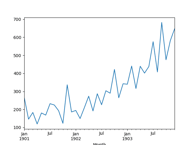
A line plot of the series is then created showing a clear increasing trend.
Line Plot of Shampoo Sales Dataset
Next, we will take a look at the LSTM configuration and test harness used in the experiment.
Experimental Test Harness
This section describes the test harness used in this tutorial.
Data Split
We will split the Shampoo Sales dataset into two parts: a training and a test set.
The first two years of data will be taken for the training dataset and the remaining one year of data will be used for the test set.
Models will be developed using the training dataset and will make predictions on the test dataset.
The persistence forecast (naive forecast) on the test dataset achieves an error of 136.761 monthly shampoo sales. This provides a lower acceptable bound of performance on the test set.
Model Evaluation
A rolling-forecast scenario will be used, also called walk-forward model validation.
Each time step of the test dataset will be walked one at a time. A model will be used to make a forecast for the time step, then the actual expected value from the test set will be taken and made available to the model for the forecast on the next time step.
This mimics a real-world scenario where new Shampoo Sales observations would be available each month and used in the forecasting of the following month.
This will be simulated by the structure of the train and test datasets.
All forecasts on the test dataset will be collected and an error score calculated to summarize the skill of the model. The root mean squared error (RMSE) will be used as it punishes large errors and results in a score that is in the same units as the forecast data, namely monthly shampoo sales.
Data Preparation
Before we can fit an LSTM model to the dataset, we must transform the data.
The following three data transforms are performed on the dataset prior to fitting a model and making a forecast.
Transform the time series data so that it is stationary. Specifically, a lag=1 differencing to remove the increasing trend in the data.
Transform the time series into a supervised learning problem. Specifically, the organization of data into input and output patterns where the observation at the previous time step is used as an input to forecast the observation at the current time step
Transform the observations to have a specific scale. Specifically, to rescale the data to values between -1 and 1 to meet the default hyperbolic tangent activation function of the LSTM model.
These transforms are inverted on forecasts to return them into their original scale before calculating and error score.
LSTM Model
We will use a base stateful LSTM model with 1 neuron fit for 1000 epochs.
A batch size of 1 is required as we will be using walk-forward validation and making one-step forecasts for each of the final 12 months of test data.
A batch size of 1 means that the model will be fit using online training (as opposed to batch training or mini-batch training). As a result, it is expected that the model fit will have some variance.
Ideally, more training epochs would be used (such as 1500), but this was truncated to 1000 to keep run times reasonable.
The model will be fit using the efficient ADAM optimization algorithm and the mean squared error loss function.
Experimental Runs
Each experimental scenario will be run 10 times.
The reason for this is that the random initial conditions for an LSTM network can result in very different results each time a given configuration is trained.
Let’s dive into the experiments.
A vs A Test
A good first experiment is to evaluate how noisy or reliable our test harness may be.
This can be evaluated by running the same experiment twice and comparing the results. This is often called an A vs A test in the world of A/B testing, and I find this name useful. The idea is to flush out any obvious faults with the experiment and get a handle on the expected variance in the mean value.
We will run an experiment with a stateful LSTM on the network twice.
The complete code listing is provided below.
This code also provides the basis for all experiments in this tutorial. Rather than re-listing it for each variation in subsequent sections, I will only list the functions that have been changed.
1
2
3
4
5
6
7
8
9
10
11
12
13
14
15
16
17
18
19
20
21
22
23
24
25
26
27
28
29
30
31
32
33
34
35
36
37
38
39
40
41
42
43
44
45
46
47
48
49
50
51
52
53
54
55
56
57
58
59
60
61
62
63
64
65
66
67
68
69
70
71
72
73
74
75
76
77
78
79
80
81
82
83
84
85
86
87
88
89
90
91
92
93
94
95
96
97
98
99
100
101
102
103
104
105
106
107
108
109
110
111
112
113
114
115
116
117
118
119
120
121
122
123
124
125
126
127
128
129
130
from pandas import DataFrame
from pandas import Series
from pandas import concat
from pandas import read_csv
from pandas import datetime
from sklearn.metrics import mean_squared_error
from sklearn.preprocessing import MinMaxScaler
from keras.models import Sequential
from keras.layers import Dense
from keras.layers import LSTM
from math import sqrt
import matplotlib
import numpy
from numpy import concatenate
# date-time parsing function for loading the dataset
def parser(x):
returndatetime.strptime('190'+x,'%Y-%m')
# frame a sequence as a supervised learning problem
Running the experiment saves the results to a file named “experiment_stateful.csv“.
Run the experiment a second time and change the filename written by the experiment to “experiment_stateful2.csv” as to not overwrite the results from the first run.
You should now have two sets of results in the current working directory in the files:
experiment_stateful.csv
experiment_stateful2.csv
We can now load and compare these two files. The script to do this is listed below.
This script loads the result files and first calculates descriptive statistics for each run.
Note: Your results may vary given the stochastic nature of the algorithm or evaluation procedure, or differences in numerical precision. Consider running the example a few times and compare the average outcome.
We can see that the mean results and standard deviation are relatively close values (around 103-106 and 7-10 respectively). This is a good sign, but not perfect. It is expected that increasing the number of repeats of the experiment from 10 to 30, 100, or even 1000 would produce near identical summary statistics.
1
2
3
4
5
6
7
8
9
stateful stateful2
count 10.000000 10.000000
mean 103.142903 106.594624
std 7.109461 10.687509
min 94.052380 91.570179
25% 96.765985 101.015403
50% 104.376252 102.425406
75% 107.753516 115.024920
max 114.958430 125.088436
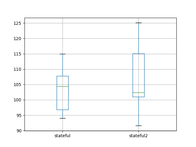
The comparison also creates a box and whisker plot to compare the two distributions.
The plot shows the 25th, 50th (median), and 75th percentile of 10 test RMSE results from each experiment. The box shows the middle 50% of the data and the green line shows the median.
The plot shows that although the descriptive statistics are reasonably close, the distributions do show some differences.
Nevertheless, the distributions do overlap and comparing means and standard deviations of different experimental setups is reasonable as long as we don’t quibble over modest differences in mean.
Box and Whisker Plot of A vs A Experimental Results
A good follow-up to this analysis is to review the standard error of the distribution with different sample sizes. This would involve first creating a larger pool of experimental runs from which to draw (100 or 1000), and would give a good idea of a robust number of repeats and an expected error on the mean when comparing results.
Stateful vs Stateless LSTMs
A good first experiment is to explore whether maintaining state in the LSTM adds value over not maintaining state.
In this section, we will contrast:
A Stateful LSTM (first result from the previous section).
A Stateless LSTM with the same configuration.
A Stateless LSTM with shuffling during training.
The benefit of LSTM networks is their ability to maintain state and learn a sequence.
Expectation 1: The expectation is that the stateful LSTM will outperform the stateless LSTM.
Shuffling of input patterns each batch or epoch is often performed to improve the generalizability of an MLP network during training. A stateless LSTM does not shuffle input patterns during training because the network aims to learn the sequence of patterns. We will test a stateless LSTM with and without shuffling.
Expectation 2: The expectation is that the stateless LSTM without shuffling will outperform the stateless LSTM with shuffling.
The code changes to the stateful LSTM example above to make it stateless involve setting stateful=False in the LSTM layer and the use of automated training epoch training rather than manual. The results are written to a new file named “experiment_stateless.csv“. The updated fit_lstm() function is listed below.
The stateless with shuffling experiment involves setting the shuffle argument to True when calling fit in the fit_lstm() function. The results from this experiment are written to the file “experiment_stateless_shuffle.csv“.
The complete updated fit_lstm() function is listed below.
Running the example first calculates and prints descriptive statistics for each of the experiments.
Note: Your results may vary given the stochastic nature of the algorithm or evaluation procedure, or differences in numerical precision. Consider running the example a few times and compare the average outcome.
The average results suggest that the stateless LSTM configurations may outperform the stateful configuration. If robust, this finding is quite surprising as it does not meet the expectation of the addition of state improving performance.
The shuffling of training samples does not appear to make a large difference to the stateless LSTM. If the result is robust, the expectation of shuffled training order on the stateless LSTM does appear to offer some benefit.
Together, these findings may further suggest that the chosen LSTM configuration is focused more on learning input-output pairs rather than dependencies within the sequence.
From these limited results alone, one would consider exploring stateless LSTMs on this problem.
1
2
3
4
5
6
7
8
9
stateful stateless stateless_shuffle
count 10.000000 10.000000 10.000000
mean 103.142903 95.661773 96.206332
std 7.109461 1.924133 2.138610
min 94.052380 94.097259 93.678941
25% 96.765985 94.290720 94.548002
50% 104.376252 95.098050 95.804411
75% 107.753516 96.092609 97.076086
max 114.958430 100.334725 99.870445
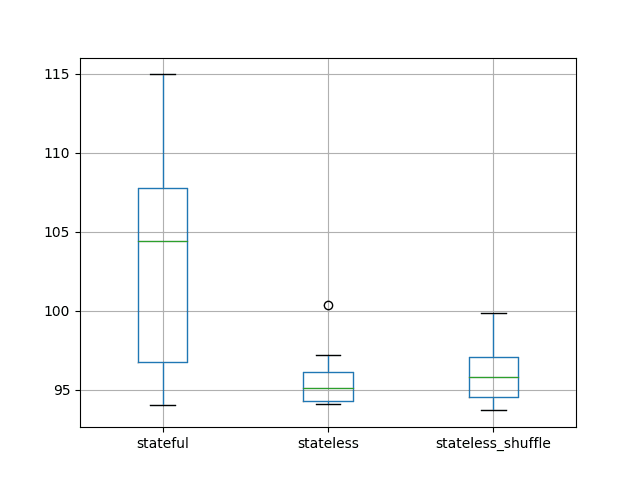
A box and whisker plot is also created to compare the distributions.
The spread of the data appears much larger with the stateful configuration compared to the stateless cases. This is also present in the descriptive statistics when we look at the standard deviation scores.
This suggests that the stateless configurations may be more stable.
Box and Whisker Plot of Test RMSE of Stateful vs Stateless LSTM Results
Stateless with Large Batch vs Stateless
A key to understanding the difference between stateful and stateless LSTMs is “when internal state is reset”.
Stateless: In the stateless LSTM configuration, internal state is reset after each training batch or each batch when making predictions.
Stateful: In the stateful LSTM configuration, internal state is only reset when the reset_state() function is called.
If this is the only difference, then it may be possible to simulate a stateful LSTM with a stateless LSTM using a large batch size.
Expectation 3: Stateless and stateful LSTMs should produce near identical results when using the same batch size.
We can do this with the Shampoo Sales dataset by truncating the training data to only 12 months and leaving the test data as 12 months. This would allow a stateless LSTM to use a batch size of 12. If training and testing were performed in a one-shot manner (one function call), then it is possible that internal state of the “stateless” LSTM would not be reset and both configurations would produce equivalent results.
We will use the stateful results from the first experiment as a starting point. The forecast_lstm() function is modified to forecast one year of observations in a single step. The experiment() function is modified to truncate the training dataset to 12 months of data, to use a batch size of 12, and to process the batched predictions returned from the forecast_lstm() function. These updated functions are listed below. Results are written to the file “experiment_stateful_batch12.csv“.
We will use the stateless LSTM configuration from the previous experiment with training pattern shuffling turned off as the starting point. The experiment uses the same forecast_lstm() and experiment() functions listed above. Results are written to the file “experiment_stateless_batch12.csv“.
After running this experiment, you will have two result files:
experiment_stateful_batch12.csv
experiment_stateless_batch12.csv
We can now compare the results from these experiments.
Running the comparison script first calculates and prints the descriptive statistics for each experiment.
Note: Your results may vary given the stochastic nature of the algorithm or evaluation procedure, or differences in numerical precision. Consider running the example a few times and compare the average outcome.
The average results for each experiment suggest equivalent results between the stateless and stateful configurations with the same batch size. This confirms our expectations.
If this result is robust, it suggests that there are no further implementation-detailed differences between stateless and stateful LSTM networks in Keras beyond when the internal state is reset.
1
2
3
4
5
6
7
8
9
stateful_batch12 stateless_batch12
count 10.000000 10.000000
mean 97.920126 97.450757
std 6.526297 5.707647
min 92.723660 91.203493
25% 94.215807 93.888928
50% 95.770862 95.640314
75% 99.338368 98.540688
max 114.567780 110.014679
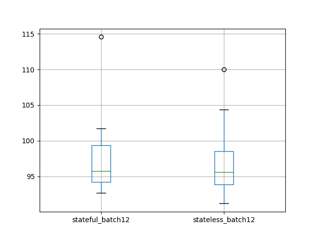
A box and whisker plot is also created to compare the distributions.
The plot confirms the story in the descriptive statistics, perhaps just highlighting variability in the experimental design.
Box and Whisker Plot of Test RMSE of Stateful vs Stateless with Large Batch Size LSTM Results
Stateful Resetting vs Stateless
Another question regarding stateful LSTMs is the best regime to perform resets to state.
Generally, we would expect that resetting the state after each presentation of the sequence would be a good idea.
Expectation 4: Resetting state after each training epoch results in better test performance.
This raises the question as to the best way to manage state when making predictions. For example, should the network be seeded with state from making predictions on the training dataset first?
Expectation 5: Seeding state in the LSTM by making predictions on the training dataset results in better test performance.
We would also expect that not resetting LSTM state between one-step predictions on the test set would be a good idea.
Expectation 6: Not resetting state between one-step predictions on the test set results in better test set performance.
There is also the question of whether or not resetting state at all is a good idea. In this section, we attempt to tease out answers to these questions.
We will again use all of the available data and a batch size of 1 for one-step forecasts.
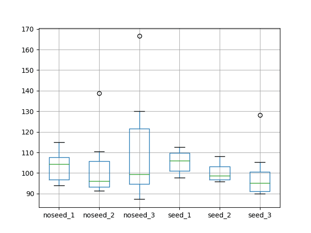
In summary, we are going to compare the following experimental setups:
No Seeding:
noseed_1: Reset state after each training epoch and not during testing (the stateful results from the first experiment in experiment_stateful.csv).
noseed_2: Reset state after each training epoch and after each one-step prediction (experiment_stateful_reset_test.csv).
noseed_3: No resets after training or making one-step predictions (experiment_stateful_noreset.csv).
Seeding:
seed_1: Reset state after each training epoch, seed state with one-step predictions on training dataset before making one-step predictions on the test dataset (experiment_stateful_seed_train.csv).
seed_2: Reset state after each training epoch, seed state with one-step predictions on training dataset before making one-step predictions on the test dataset and reset state after each one-step prediction on train and test sets (experiment_stateful_seed_train_resets.csv).
seed_3: Seed on training dataset before making one-step predictions, no resets during training on predictions (experiment_stateful_seed_train_no_resets.csv).
The stateful experiment code from the first “A vs A” experiment is used as a base.
The modifications needed for the various resetting/no-resetting and seeding/no-seeding are listed below.
We can update the forecast_lstm() function to update after each test by adding a call to reset_states() on the model after each prediction is made. The updated forecast_lstm() function is listed below.
1
2
3
4
5
6
# make a one-step forecast
def forecast_lstm(model,batch_size,X):
X=X.reshape(1,1,len(X))
yhat=model.predict(X,batch_size=batch_size)
model.reset_states()
returnyhat[0,0]
We can update the fit_lstm() function to not reset after each epoch by removing the call to reset_states(). The complete function is listed below.
We can seed the state of LSTM after training with the state from making predictions on the training dataset by looping through the training dataset and making one-step forecasts. This can be added to the run() function before making one-step forecasts on the test dataset. The updated run() function is listed below.
Running the comparison prints descriptive statistics for each set of results.
Note: Your results may vary given the stochastic nature of the algorithm or evaluation procedure, or differences in numerical precision. Consider running the example a few times and compare the average outcome.
The results for no seeding suggest perhaps little difference between resetting after each prediction on the test dataset and not. This suggests any state built up from prediction to prediction is not adding value, or that this state is implicitly cleared by the Keras API. This was a surprising result.
The results on the no-seed case also suggest that having no resets during training results in worse on average performance with larger variance than resetting the state at the end of each epoch. This confirms the expectation that resetting the state at the end of each training epoch is a good practice.
The average results from the seed experiments suggest that seeding LSTM state with predictions on the training dataset before making predictions on the test dataset is neutral, if not resulting in slightly worse performance.
Resetting state after each prediction on the train and test sets seem to result in slightly better performance, whereas not resetting state during training or testing seems to result in the best performance.
These results regarding seeding are surprising, but we should note that the mean values are all within a test RMSE of 5 monthly shampoo sales and could be statistical noise.
max 114.958430 138.752321 166.527902 112.691046 108.070145 128.261354
A box and whisker plot is also created to compare the distributions.
The plot tells the same story as the descriptive statistics. It highlights the increased spread when no resets are used on the stateless LSTM without seeding. It also highlights the general tight spread on the experiments that seed the state of the LSTM with predictions on the training dataset.
Box and Whisker Plot of Test RMSE of Reset Regimes in Stateful LSTMs
Review of Findings
In this section, we recap the findings throughout this tutorial.
10 repeats of an experiment with the chosen configuration results in some variation in the mean and standard deviation of the test RMSE of about 3 monthly shampoo sales. More repeats would be expected to tighten this up.
The stateless LSTM with the same configuration may perform better on this problem than the stateful version.
Not shuffling training patterns with the stateless LSTM may result in slightly better performance.
When a large batch size is used, a stateful LSTM can be simulated with a stateless LSTM.
Resetting state when making one-step predictions with a stateful LSTM may improve performance on the test set.
Seeding state in a stateful LSTM by making predictions on the training dataset before making predictions on the test set does not result in an obvious improvement in performance on the test set.
Fitting a stateful LSTM and seeding it on the training dataset and not performing any resetting of state during training or prediction may result in better performance on the test set.
It must be noted that these findings should be made more robust by increasing the number of repeats of each experiment and confirming the differences are significant using statistical significance tests.
It should also be noted that these results apply to this specific problem, the way it was framed, and the chosen LSTM configuration parameters including topology, batch size, and training epochs.
Summary
In this tutorial, you discovered how to investigate the impact of using stateful vs stateless LSTM networks for time series forecasting in Python with Keras.
Specifically, you learned:
How to compare stateless vs stateful LSTM networks for time series forecasting.
How to confirm the equivalence of stateless LSTMs and stateful LSTMs with a large batch size.
How to evaluate the impact of when LSTM state is reset during training and making predictions with LSTM networks for time series forecasting.
Do you have any questions? Ask your questions in the comments and I will do my best to answer.
Develop Deep Learning models for Time Series Today!
How do we deal with the case when there the data has multiple features/labels per time series that we have suspicion have strong correlation (assumed to be strong). For example:
YR Month Production Sales
1999 1 Shampoo $400
1999 1 Conditioner $300
1999 2 Shampoo $410
1999 2 Conditioner $305
And so in this case we would like to be build one single model to predict Shampoo/Conditioner sales.
Is this configured by setting to the batch to 2 stateful (or 24 in the case of stateless) or am I looking at this all wrong?
Hi Jason,
I follow your blog entries regarding lstms and time series quite a while and I like them really well. I have a question about something that does not fit 100% on the blog posts, but maybe you would like to share your ideas with me as I am relatively new in this area. I have a record consisting of 61 multivariate timeseries. Each time I have assigned a label in the preprocessing (0, 1 or 2).
I would like to make a multi-class classification with lstm’s.
As the starting point, I used the following:
and learn with a batch size of 1 over 150 epochs. The dataset is divided into a training and test set.
I already have an accuracy of 97%. I think this is partly due to the data distribution, because label one occurs at about 94% and the other two about equally often. Nevertheless, it’s better than ever predict label one.
In the next steps, I will first let the batch size vary, and manage the memory cell.
Do you have other suggestions to increase the accuracy or any other things to do differently based on your experience? Or is there a reason to change the problem rather to a forecast problem?
Generally I have 3 problems:
1) The predicted labels are not 100% overlapping with the true labels. What I think is not quite so bad
2) I have something like jumping / oscillating values between two labels. I think that this will be improved with other parameter settings. But generally is there a recommended standard technique to treat these labels again, as for example like the moving average?
3)Completely wrongly labeled areas
Would you recommend to adjust the distribution of the data, so that each label equally often occur?
Many greetings,
chris
If your classes are not balanced, consider using a different measure than accuracy to get a true idea of the model skill, like a confusion matrix, logloss or AUC.
Try to quantify exactly what type of errors the model is making.
If there is conflict in the data, find a way to resolve it, perhaps the time axis or another variable can be used (feature engineering).
Good Morning, thanks for your quick reply. I started using the confusion matrix yesterday ????. At the log loss I haven’t thought.
The feature engineering idea sounds really good,since I always have corridors of the same size for the 0 and 2 labels. I think, I’ll look at the rebalancing later and first try the other appoaches. Thanks for the advices! I will keep you up to date.
Hi Jason,
thanks again for the last tips.
Currently I get quite good results. The AUC for each of my three classes is already between 96-99 and also the F-Measure is better than in all models used so far.
I still have a few jumps in the labels, but I think I can certainly reduce them.
I now have the problem that I currently use 37 or even 62 different features.
I would like to perform a feature selection. Unfortunately, I have found nothing for keras / neural networks. Do you already know something that can be used for neural networks or even has experience with it? Or is that no standard practice for NN? Thank you
Hi Jason, when running the second ( large ) piece of code using PyCharm I get “UnicodeDecodeError: ‘utf-8’ codec can’t decode byte 0xf6 in position 22: invalid start byte”, it seems to work using Spyder , however
best regards George
Great post! Maybe you would be able to help me with my problem?
I have a sequential data representing moving targets recorded by a radar. Sequences of some targets are longer than the others.
For example,
I have labeled data of cars and their velocities, accelerations etc.
‘c’ represents a car with a 3-dimensional feature vector, age is the number of times a target was recorded by the radar. Label means different types of cars such as truck etc.
c1 = [2,3,5], label = 0, age = 1
c2 = [2,4,7], label = 1, age = 1
c3 = [5,6,3], label = 2, age = 1
c1 = [4,5,7], label = 0, age = 2
c1 = [5,7,8], label = 0, age = 3
c2 = [6,7,4], label = 1, age = 2
c1 = [1,3,8], label = 0, age = 4
c3 = [5,6,3], label = 2, age = 2
As you can see, the sequences of some targets are longer than the others.
My question is how could I account for it while creating an LSTM model?
For example, by choosing window size 2, I would get [c1, c2, c3], [c2, c3, c1] and so on…
What happens to the labels in this case?
This is a classification problem so would stateful or stateless network be more appropriate?
Hi Jason! I have some second thoughts about the stateless lstm.
The main purpose of the LSTM is to utilize its memory property. Based on that what is the point of a stateless LSTM to exist? Don’t we “convert” it into a simple NN by doing that?
In other words.. Does the stateless use of LSTM aim to model the sequences (window) in the input data – if we apply shuffle=False in the fit layer in keras – (eg. for a window of 10 time steps capture any pattern between 10-character words)? If yes why don’t we convert the initial input data to match the form of the sequencers under inspection and then use a plain NN (by adding extra columns to the original dataset that are shifted)?
If we choose to have shuffle = True then we are losing any information that could be found in our data (e.g. time series data – sequences), don’t we? In that case I would expect in to behave similarly to a plain NN and get the same results between the two by setting the same random seed.
Regarding the shuffling according to the documentation “shuffle: boolean or str (for ‘batch’). Whether to shuffle the samples at each epoch”. So it first resamples the data (i.e. changes the original order) and then on the new order creates the batches. Do I get it right?
Let me restate my previous question because I might have confused you. Suppose the dataset has only one variable X and one label Y. I actually want to know whether a stateless LSTM of batch size say 5 and timestep 1 is equivalent to a NN that will get as input X and X.shift(1) (so in total 2 inputs (2 columns) although they point to the same original X column of my dataset and batch size also 5.
Thanks in advance and congrats on your helpful website!
Even if you frame the sequence problem the same way for LSTMs and MLPs, the units inside each network are different (e.g. LSTMs have memory and gates). In turn, results will probably differ.
I would encourage you to test both types of networks on your problem, and most importantly, brainstorm many different ways to frame your sequence prediction problem to see which works best.
“Transform the observations to have a specific scale. Specifically, to rescale the data to values between -1 and 1 to meet the default hyperbolic tangent activation function of the LSTM model.”
I have often ran into this comment where data should be prepared to fit the Y range of the activation function. Consequently, I’ve been trying to find the intuition or theoretical reason behind such transformation, but could not find any besides discussions on SO.
I would much appreciate if you could provide your wisdom regarding following questions.
a) why such transformation is necessary
b) is the transformation applicable to all other activation functions (e.g. [0,1] for sigmoid and on)?
Generally, normalizing or standardizing data doe help with neural nets. I would recommend testing with and without it and see how it impacts model skill.
Hi Jason,
what do you think of using a callback to reset states so that it is possible to use model.fit() on the entire set? Is there any reason to not do this?
Hello,
Thanks for the wonderful post .
I have a couple of questions on the way these long sequences have to be handled when traininig a LSTM network :
Suppose I have a sequence classification task for which I have a set of 100 sequences with each sequence of varying length in the range 1000 – 2000 (samples). I would need the sequence classification task to identify sequences at regular intervals say every 10 or 20 samples within a sequence
a. How do I preprocess the data i.e break down the data in to subsequences for training ? Is the sub-sequence length based on the dependency of output over the number of input Samples ?
b. If my output of Sequence classification depends on say last 20 samples within a sequence, how do I Split the input data sequence for training ?
i.Should it be this way : Overlapping sub-sequences and Stateless – LSTM
s1_1,s1_2,…….s1_20
s1_2,s1_3……..s1_21
s1_3,s1_4……..s1_22
ii.Or Should it be this way : Non-overlapping sub-sequences and Stateful – LSTM
s1_1,s1_2,…….s1_20
s1_21,s1_22……..s1_40
s1_41,s1_42……..s1_60
Which among the above mentioned options(i and ii)is right? and Why ?
Does the approach ii. learn dependencies longer than 20 samples … as the state is carry forwarded after each sub-sequence? If yes till what extent (number of samples … say 60 or 100)?
c. If my output of Sequence classification depends on say last 900 samples within a sequence, can the LSTM solve/address this problem ? If yes what would the split of a single training sequence be in such a situation and what would be the LSTM implementation be(Stateful or Stateless)?
I would further encourage you to explore many different framings of your sequence classification problem and see what works best for your specific data.
Thanks alot for your tutorials they are very helpful.
I am trying to implement the stateless LSTM without shuffle. I basically used your code as it is with only the changes that you suggested, but unfortunately i am getting the following error:
GPU sync failed
By any chance do you have any idea why am I getting this error?
I am working on an industry problem in which we are trying to predict scrap rates in a manufacturing line based on large datasets (machine data, sensor data, …). One approach is to model the problem as a time series (sequence) regression problem in RNNs. I am frequently using your blog as incredily helpful resource (thanks!).
The prototyping is done in Keras and therefore, I have the following question:
Two parameters suggest to influence sequence learning problems:
– batch_size in model.fit(batch_size)
– time_steps in layers.LSTM(input_shape(samples,time_steps,obs)
-> If batch_size < time_steps , doesn't the internal state get reset too frequently and causes a problem with the BPTT?
As an example, suppose we have a sequence of length 50 (time_steps=50) and a training batch size of 25 e.g. for stochastic gradient descent (batch_size=25). Even though TBPTT(50,50) is set up to learn sequence patterns from 50 time steps, can the internal state keep the information?
Oh, I will try to summarize here so if something not clear please tell me.
First, i have solved my problem in the link thanks to your tutorial on saving weights for prediction in different batch size LSTM. yet i have issue in accuracy.
second, i have 4 features, that i am using the last one in training and also as a target. thanks to your tutorials i was able to reshape the data and make the below stateful architecture, note its window size of 10
# fit network
for i in range(len(X_train)):
if X_train[i].shape[0] == 250:
model.fit(X_train[i], y_train[i], epochs=n_epoch, batch_size=n_batch, verbose=1, shuffle=False)
#model.reset_states()
note that commenting the reset_states or not doesn’t affect the accuracy
Third, i am not sure if i am calculating the accuracy and loss right, also if i am using the proper optimizer, also what activation functions to use, should i stack more LSTM. why stateful doesn’t affect the learning.
Also the last feature has large positive and negative values, not more than 1000. so what is the proper way to normalize that.
i tried to normalize using the below line, but nothing changed, same 0% accuracy!!
m15 = m15.assign(NormDirHeight=(m15[‘DirHeight’]-m15[‘DirHeight’].mean())/m15[‘DirHeight’].std())
First, Thank you so much and your tutorials are super awesome and super fun, this is something i wanted to say.
Sorry for dumping the log here
Okay, so using mae for metrics, i got the below, without MinMaxScaler
But if i am not calculating accuracy how could i know that this is good or bad ?
Also why is it always the same either reset_states() or without it ?
The Stateful is very confusing, nevertheless going from here to predicting multiple steps using TimeDistrubed is a whole new fun journey xD
I was able to show the actual and predicted after applying inverse transform, clearly its a mess. Is it the data or the architecture, how could i know ?
Okay, i have one last question, How could i know that the problem is not in my data ?
i mean that i always get the same bad accuracy, is it the data ? is there something that check the consistency of the data that it would be valid to make a regression function for it with LSTM ?
Thank you so much, i have read the article carefully, analyzed how much of it i did and which steps did i skip, and put an action plan. really great blog and thanks for your nice and fast replies)
Hi Jason,
In Stateful model, callbacks of Keras(EarlyStopping, ReduceLROnPlateau, and ModelCheckpoint) not working.
As we are resetting the states after each iteration and in between each iteration there is only one epoch, hence Keras is not able to find logs of previous epochs, hence not able to apply above mention callbacks.
So, How can I implement EarlyStopping, ReduceLROnPlateau, and ModelCheckpoint?
If you are driving the epochs manually, then the perhaps callbacks are not needed (just an idea?), you can run their operations manually as well. E.g. evaluate the model and see if you the next iteration is required or not.
Great tutorial. I just have one question that in step 3 of data preparation you said that:
“Transform the observations to have a specific scale. Specifically, to rescale the data to values between -1 and 1 to meet the default hyperbolic tangent activation function of the LSTM model”
Why are you scaling your input between -1 and 1? tanh has domain of all real line and range from -1 to 1 so why to scale between -1 and 1 and not [0,1] or any other? I know that the active region for tanh is [-2, 2] but I don’t understand your logic.
A great post yet once again. I have a doubt w.r.t. the sample size while prediction. Let’s say during training my batch_size=32 and being a stateful=True network, I need to specify batch_size in the input layer itself.
Now during prediction, it expects the batch_size to be the same as used while training. But in case if I want to predict for records less than 32, do I need to pad the whole sequence until size 32? Thanks in advance.
Dear Dr Jason,
Thank you very much for your tutorial.
I jumped into an error, and could not figure it out what went wrong,
When I tried to load these files: “experiment_stateful.csv” and “experiment_stateful2.csv”
I load it as your script but it throw the error “ValueError: Cannot set a frame with no defined index and a value that cannot be converted to a Series” at these lines
[for name in filenames:
results[name[11:-4]] = read_csv(name, header=0)]
I am using panda 1.0.1 and Python 3.7, sorry but I am relatively new to this area, I hope that you can help with the explanation as well as suggestion for other supplement tutorials.
Thank you for your reply, the 1st two parts of the code ran smoothly and gave me 2 expected output files. However, at this line:
results[name[11:-4]] = read_csv(name, header=0)
I suppose that the index[11:-4] includes a no defined index as the shown error. Would you mind suggest me what may goes wrong or where to look further here.
Thanks in advance.
Thank you for your reply. I did run the first part, and got the csv files since my 1st comment, however in the loading files for comparing part, I jumped into the mentioned error. Again, sorry for taking ur time due to my lack of exp in this field. I managed to modify the code and display it with pandas concat method as follow:
for name in filenames:
df = read_csv(name, header=0)
df[‘name’] = name
results = pd.concat([results, df])
# describe all results
print(results.describe())
# box and whisker plot
results.boxplot(by=’name’)
pyplot.show()
Could you help me to understand what may go wrong with “results[name[11:-4]]” in your scripts ?
Something I’m missing here. I get that this is model is trying to predict a “known” sale amount. What I don’t understand is how you would use this to forecast beyond the “known” sale history? How do you use the model to continue making predictions beyond the last “known” sale date?
Hi, I did not see anyone evaluating loss function on validation data during training using stateful LSTM yet. Is it even possible? I am not sure how state is handled, because when using stateful network you will probably need different states for training and validation data, is that right?
So after each epoch resetting model and evaluate on set of validation data? Makes sense, but I am afraid that it will make training painfully slow in Keras.
Thank you for an amazing article. I have learnt a lot from it. I have a question when the problem is a multivariate one. My output (say O1) looks very similar to the one shown here, with its own trend and seasonality but my input signals are different (say I1, I2). In this scenario, does it make sense to make all the input and output signals stationary (irrespective of whether I1 and I2 have seasonality) and try through stateful LSTM or would you recommend another approach?
Looking forward to your response.
Thank you for your response. I will go ahead and try the approach. One small follow up questuin though. I have multiple excel files with such time series data. Could you kindly help me in understanding how to use these multiple data files for training the LSTM network? Stitching them together causes a sudden drop because the end of one file has a much lower value than the beginning of the next file. So, Im not sure if that is the right way to do it. I would really appreciate your help on this.
For your initial stateful vs stateless attempt, you seem to get better results for stateless, but then you proceed to show that they give the same results when batch size is the same. But for the initial attempt, you don’t show the batch size for the two. What did you specify for batch size for the stateful and stateless in the first attempt?
Thanks a lot for knowledge sharing!!!
I have a question regarding one of the experiments where it was concluded that for a stateful model, resetting the state after every epoch turns better than stateless.
In this case, how different is this than a stateless model as we are explicitly resetting the state?
If we are explicitly resetting the state of a stateful model, then we are essentially doing what a stateless would have done. So, why we are using stateful here and not stateless?
thanks a lot for article!
but i miss important things:
why you scale Y(target) also? is it nessesary?
i was sure – we need scale to -1,1 or 0,1 only X…..
very thank, James, now it is clear about scaling!
one more question about this article: what is the reason of using “difference” func ? i was hope the model must predict any trends itself? why we need prepare by shifting X this way?
….also may be you can advise where to further read more about peculiarities of use -LSTM/TimeDistributed/return_sequences=True w.r.t. modeling typicial target trend (very similar to sin() function – i can see period)
In fact I am getting “TypeError: reset_states() got an unexpected keyword argument ‘states'” wehn passing model.reset_states(states=None) at the begining of the “File” loop.
Hi Mike…Did you copy and paste the code or type it in? Also, you may want to try it in Google Colab and see if you experience the same issue. I find this helpful to rule out typing mistakes.


Hi Jason,
Great subject and article.
How do we deal with the case when there the data has multiple features/labels per time series that we have suspicion have strong correlation (assumed to be strong). For example:
YR Month Production Sales
1999 1 Shampoo $400
1999 1 Conditioner $300
1999 2 Shampoo $410
1999 2 Conditioner $305
And so in this case we would like to be build one single model to predict Shampoo/Conditioner sales.
Is this configured by setting to the batch to 2 stateful (or 24 in the case of stateless) or am I looking at this all wrong?
Same as any other algorithm.
Explore using all features in the model, explore removing highly corrected features and see how that affects the model.
Hi Jason,
I follow your blog entries regarding lstms and time series quite a while and I like them really well. I have a question about something that does not fit 100% on the blog posts, but maybe you would like to share your ideas with me as I am relatively new in this area. I have a record consisting of 61 multivariate timeseries. Each time I have assigned a label in the preprocessing (0, 1 or 2).
I would like to make a multi-class classification with lstm’s.
As the starting point, I used the following:
model.add(LSTM(61, input_shape=(1, 61)))
model.add(Dense(3, activation=’softmax’))
model.compile(loss=’categorical_crossentropy’, optimizer=’adam’, metrics=[‘accuracy’])
and learn with a batch size of 1 over 150 epochs. The dataset is divided into a training and test set.
I already have an accuracy of 97%. I think this is partly due to the data distribution, because label one occurs at about 94% and the other two about equally often. Nevertheless, it’s better than ever predict label one.
In the next steps, I will first let the batch size vary, and manage the memory cell.
Do you have other suggestions to increase the accuracy or any other things to do differently based on your experience? Or is there a reason to change the problem rather to a forecast problem?
Generally I have 3 problems:
1) The predicted labels are not 100% overlapping with the true labels. What I think is not quite so bad
2) I have something like jumping / oscillating values between two labels. I think that this will be improved with other parameter settings. But generally is there a recommended standard technique to treat these labels again, as for example like the moving average?
3)Completely wrongly labeled areas
Would you recommend to adjust the distribution of the data, so that each label equally often occur?
Many greetings,
chris
Hi Chris,
If your classes are not balanced, consider using a different measure than accuracy to get a true idea of the model skill, like a confusion matrix, logloss or AUC.
Try to quantify exactly what type of errors the model is making.
If there is conflict in the data, find a way to resolve it, perhaps the time axis or another variable can be used (feature engineering).
Most methods I know for rebalancing data are not for time series data, for example:
https://machinelearningmastery.com/tactics-to-combat-imbalanced-classes-in-your-machine-learning-dataset/
I do have a suite of general ideas for lifting the skill of deep learning models here:
https://machinelearningmastery.com/improve-deep-learning-performance/
I hope that helps as a start.
Good Morning, thanks for your quick reply. I started using the confusion matrix yesterday ????. At the log loss I haven’t thought.
The feature engineering idea sounds really good,since I always have corridors of the same size for the 0 and 2 labels. I think, I’ll look at the rebalancing later and first try the other appoaches. Thanks for the advices! I will keep you up to date.
Nice work, let me know how you go.
Hi Jason,
thanks again for the last tips.
Currently I get quite good results. The AUC for each of my three classes is already between 96-99 and also the F-Measure is better than in all models used so far.
I still have a few jumps in the labels, but I think I can certainly reduce them.
I now have the problem that I currently use 37 or even 62 different features.
I would like to perform a feature selection. Unfortunately, I have found nothing for keras / neural networks. Do you already know something that can be used for neural networks or even has experience with it? Or is that no standard practice for NN? Thank you
Hi chris,
I would recommend performing feature selection up-front (prior to modeling) using sklearn:
https://machinelearningmastery.com/feature-selection-machine-learning-python/
Hi Jason, when running the second ( large ) piece of code using PyCharm I get “UnicodeDecodeError: ‘utf-8’ codec can’t decode byte 0xf6 in position 22: invalid start byte”, it seems to work using Spyder , however
best regards George
I recommend running all code from the command line.
Hi Jason,
Great post! Maybe you would be able to help me with my problem?
I have a sequential data representing moving targets recorded by a radar. Sequences of some targets are longer than the others.
For example,
I have labeled data of cars and their velocities, accelerations etc.
‘c’ represents a car with a 3-dimensional feature vector, age is the number of times a target was recorded by the radar. Label means different types of cars such as truck etc.
c1 = [2,3,5], label = 0, age = 1
c2 = [2,4,7], label = 1, age = 1
c3 = [5,6,3], label = 2, age = 1
c1 = [4,5,7], label = 0, age = 2
c1 = [5,7,8], label = 0, age = 3
c2 = [6,7,4], label = 1, age = 2
c1 = [1,3,8], label = 0, age = 4
c3 = [5,6,3], label = 2, age = 2
As you can see, the sequences of some targets are longer than the others.
My question is how could I account for it while creating an LSTM model?
For example, by choosing window size 2, I would get [c1, c2, c3], [c2, c3, c1] and so on…
What happens to the labels in this case?
This is a classification problem so would stateful or stateless network be more appropriate?
Thank you,
Kris
Sorry, I’m not sure I follow.
Consider providing the entire sequences as input time steps.
Also consider padding sequences to make the same length if the number of time steps differ.
Hi Jason! I have some second thoughts about the stateless lstm.
The main purpose of the LSTM is to utilize its memory property. Based on that what is the point of a stateless LSTM to exist? Don’t we “convert” it into a simple NN by doing that?
In other words.. Does the stateless use of LSTM aim to model the sequences (window) in the input data – if we apply shuffle=False in the fit layer in keras – (eg. for a window of 10 time steps capture any pattern between 10-character words)? If yes why don’t we convert the initial input data to match the form of the sequencers under inspection and then use a plain NN (by adding extra columns to the original dataset that are shifted)?
If we choose to have shuffle = True then we are losing any information that could be found in our data (e.g. time series data – sequences), don’t we? In that case I would expect in to behave similarly to a plain NN and get the same results between the two by setting the same random seed.
Am I missing something in my thinking?
The “stateless” LSTM just means that internal state is reset at the end of each batch, which works well in practice on many problems.
Really, maintaining state is part of the trade-off in backprop through time and input sequence length.
Shuffle applies to samples within a batch. BPTT really looks at time steps within a sample, then averages the gradient across the batch.
Does that help?
Regarding the shuffling according to the documentation “shuffle: boolean or str (for ‘batch’). Whether to shuffle the samples at each epoch”. So it first resamples the data (i.e. changes the original order) and then on the new order creates the batches. Do I get it right?
Let me restate my previous question because I might have confused you. Suppose the dataset has only one variable X and one label Y. I actually want to know whether a stateless LSTM of batch size say 5 and timestep 1 is equivalent to a NN that will get as input X and X.shift(1) (so in total 2 inputs (2 columns) although they point to the same original X column of my dataset and batch size also 5.
Thanks in advance and congrats on your helpful website!
Even if you frame the sequence problem the same way for LSTMs and MLPs, the units inside each network are different (e.g. LSTMs have memory and gates). In turn, results will probably differ.
I would encourage you to test both types of networks on your problem, and most importantly, brainstorm many different ways to frame your sequence prediction problem to see which works best.
My question doesn’t have much to do with LSTM.
“Transform the observations to have a specific scale. Specifically, to rescale the data to values between -1 and 1 to meet the default hyperbolic tangent activation function of the LSTM model.”
I have often ran into this comment where data should be prepared to fit the Y range of the activation function. Consequently, I’ve been trying to find the intuition or theoretical reason behind such transformation, but could not find any besides discussions on SO.
I would much appreciate if you could provide your wisdom regarding following questions.
a) why such transformation is necessary
b) is the transformation applicable to all other activation functions (e.g. [0,1] for sigmoid and on)?
Sincerely,
YJ
Generally, normalizing or standardizing data doe help with neural nets. I would recommend testing with and without it and see how it impacts model skill.
Hi Jason,
what do you think of using a callback to reset states so that it is possible to use model.fit() on the entire set? Is there any reason to not do this?
Best regards
If it’s a good fit for your model/setup, go for it.
Hello,
Thanks for the wonderful post .
I have a couple of questions on the way these long sequences have to be handled when traininig a LSTM network :
Suppose I have a sequence classification task for which I have a set of 100 sequences with each sequence of varying length in the range 1000 – 2000 (samples). I would need the sequence classification task to identify sequences at regular intervals say every 10 or 20 samples within a sequence
Input Sequences :
Sequence 1 : s1_1,s1_2,s1_3………………….s1_1000
Sequence 2 : s2_1,s2_2,s2_3………………….s2_1500
Sequence 3 : s3_1,s3_2,s3_3………………….s3_2000
.
.
.
Sequence 100 : s100_1,s100_2,s100_3………………….s100_1100
a. How do I preprocess the data i.e break down the data in to subsequences for training ? Is the sub-sequence length based on the dependency of output over the number of input Samples ?
b. If my output of Sequence classification depends on say last 20 samples within a sequence, how do I Split the input data sequence for training ?
i.Should it be this way : Overlapping sub-sequences and Stateless – LSTM
s1_1,s1_2,…….s1_20
s1_2,s1_3……..s1_21
s1_3,s1_4……..s1_22
ii.Or Should it be this way : Non-overlapping sub-sequences and Stateful – LSTM
s1_1,s1_2,…….s1_20
s1_21,s1_22……..s1_40
s1_41,s1_42……..s1_60
Which among the above mentioned options(i and ii)is right? and Why ?
Does the approach ii. learn dependencies longer than 20 samples … as the state is carry forwarded after each sub-sequence? If yes till what extent (number of samples … say 60 or 100)?
c. If my output of Sequence classification depends on say last 900 samples within a sequence, can the LSTM solve/address this problem ? If yes what would the split of a single training sequence be in such a situation and what would be the LSTM implementation be(Stateful or Stateless)?
This post will give you ideas on how to prepare your data:
https://machinelearningmastery.com/reshape-input-data-long-short-term-memory-networks-keras/
And this post:
https://machinelearningmastery.com/prepare-univariate-time-series-data-long-short-term-memory-networks/
I think you mean 20 time steps, not 20 samples.
I would further encourage you to explore many different framings of your sequence classification problem and see what works best for your specific data.
Hi Dr. Jason,
Thanks alot for your tutorials they are very helpful.
I am trying to implement the stateless LSTM without shuffle. I basically used your code as it is with only the changes that you suggested, but unfortunately i am getting the following error:
GPU sync failed
By any chance do you have any idea why am I getting this error?
Thank you
Nat
Looks like an issue with your Python environment. Perhaps try posting the error to stackoverflow?
Hi Jason,
I am working on an industry problem in which we are trying to predict scrap rates in a manufacturing line based on large datasets (machine data, sensor data, …). One approach is to model the problem as a time series (sequence) regression problem in RNNs. I am frequently using your blog as incredily helpful resource (thanks!).
The prototyping is done in Keras and therefore, I have the following question:
Two parameters suggest to influence sequence learning problems:
– batch_size in model.fit(batch_size)
– time_steps in layers.LSTM(input_shape(samples,time_steps,obs)
-> If batch_size < time_steps , doesn't the internal state get reset too frequently and causes a problem with the BPTT?
As an example, suppose we have a sequence of length 50 (time_steps=50) and a training batch size of 25 e.g. for stochastic gradient descent (batch_size=25). Even though TBPTT(50,50) is set up to learn sequence patterns from 50 time steps, can the internal state keep the information?
Thanks much and regards from Germany
Max
Time steps and batch size are not related. Batch size covers the number of samples, where time steps refers to one sample.
Does that help?
Hi Jason,
What about variable batch size for LSTM stateful
https://stackoverflow.com/questions/53489606/keras-variable-batch-size-for-stateful-lstm
Perhaps you can summarize the content of the link for me?
Oh, I will try to summarize here so if something not clear please tell me.
First, i have solved my problem in the link thanks to your tutorial on saving weights for prediction in different batch size LSTM. yet i have issue in accuracy.
second, i have 4 features, that i am using the last one in training and also as a target. thanks to your tutorials i was able to reshape the data and make the below stateful architecture, note its window size of 10
n_batch = X_train[0].shape[0]
n_epoch = 25
n_neurons = 256
model = Sequential()
model.add(LSTM(n_neurons, batch_input_shape=(n_batch, X_train[0].shape[1], X_train[0].shape[2]), stateful=True))
model.add(Dense(1))
model.compile(loss=’mae’, optimizer=’adam’, metrics=[‘accuracy’])
# fit network
for i in range(len(X_train)):
if X_train[i].shape[0] == 250:
model.fit(X_train[i], y_train[i], epochs=n_epoch, batch_size=n_batch, verbose=1, shuffle=False)
#model.reset_states()
note that commenting the reset_states or not doesn’t affect the accuracy
Third, i am not sure if i am calculating the accuracy and loss right, also if i am using the proper optimizer, also what activation functions to use, should i stack more LSTM. why stateful doesn’t affect the learning.
Also the last feature has large positive and negative values, not more than 1000. so what is the proper way to normalize that.
i tried to normalize using the below line, but nothing changed, same 0% accuracy!!
m15 = m15.assign(NormDirHeight=(m15[‘DirHeight’]-m15[‘DirHeight’].mean())/m15[‘DirHeight’].std())
If your problem is regression (predicting a quantity instead of a label), you cannot calculate accuracy, more here:
https://machinelearningmastery.com/classification-versus-regression-in-machine-learning/
Perhaps normalize the data using the MinMaxScaler from the scikit-learn library?
First, Thank you so much and your tutorials are super awesome and super fun, this is something i wanted to say.
Sorry for dumping the log here
Okay, so using mae for metrics, i got the below, without MinMaxScaler
Epoch 1/25
250/250 [==============================] – 1s 3ms/step – loss: 140.9831 – mean_absolute_error: 140.9831
Epoch 2/25
250/250 [==============================] – 0s 440us/step – loss: 140.9362 – mean_absolute_error: 140.9362
Epoch 3/25
250/250 [==============================] – 0s 464us/step – loss: 140.8762 – mean_absolute_error: 140.8762
Epoch 4/25
250/250 [==============================] – 0s 456us/step – loss: 140.8182 – mean_absolute_error: 140.8182
Epoch 5/25
250/250 [==============================] – 0s 464us/step – loss: 140.7660 – mean_absolute_error: 140.7660
Epoch 6/25
250/250 [==============================] – 0s 440us/step – loss: 140.7117 – mean_absolute_error: 140.7117
Epoch 7/25
250/250 [==============================] – 0s 456us/step – loss: 140.6606 – mean_absolute_error: 140.6606
Epoch 8/25
250/250 [==============================] – 0s 440us/step – loss: 140.6121 – mean_absolute_error: 140.6121
Epoch 9/25
250/250 [==============================] – 0s 512us/step – loss: 140.5622 – mean_absolute_error: 140.5622
Epoch 10/25
Okay, so using mae for accuracy metrics, i got the below, with MinMaxScaler (-1,1)
Epoch 1/25
250/250 [==============================] – 1s 3ms/step – loss: 0.0601 – mean_absolute_error: 0.0601
Epoch 2/25
250/250 [==============================] – 0s 444us/step – loss: 0.1010 – mean_absolute_error: 0.1010
Epoch 3/25
250/250 [==============================] – 0s 456us/step – loss: 0.0610 – mean_absolute_error: 0.0610
Epoch 4/25
250/250 [==============================] – 0s 456us/step – loss: 0.0732 – mean_absolute_error: 0.0732
Epoch 5/25
250/250 [==============================] – 0s 480us/step – loss: 0.0759 – mean_absolute_error: 0.0759
Epoch 6/25
250/250 [==============================] – 0s 524us/step – loss: 0.0619 – mean_absolute_error: 0.0619
Epoch 7/25
250/250 [==============================] – 0s 480us/step – loss: 0.0597 – mean_absolute_error: 0.0597
Epoch 8/25
250/250 [==============================] – 0s 484us/step – loss: 0.0613 – mean_absolute_error: 0.0613
Epoch 9/25
But if i am not calculating accuracy how could i know that this is good or bad ?
Also why is it always the same either reset_states() or without it ?
The Stateful is very confusing, nevertheless going from here to predicting multiple steps using TimeDistrubed is a whole new fun journey xD
Good question, I answer it here:
https://machinelearningmastery.com/faq/single-faq/how-to-know-if-a-model-has-good-performance
I was able to show the actual and predicted after applying inverse transform, clearly its a mess. Is it the data or the architecture, how could i know ?
>Expected=182.0, Predicted=-3.9
>Expected=-73.0, Predicted=-31.3
>Expected=-49.0, Predicted=-10.6
>Expected=48.0, Predicted=-7.8
>Expected=46.0, Predicted=-12.8
>Expected=-41.0, Predicted=-19.9
>Expected=-66.0, Predicted=-13.6
>Expected=22.0, Predicted=-1.8
>Expected=87.0, Predicted=-14.1
>Expected=47.0, Predicted=-33.3
>Expected=31.0, Predicted=-30.5
Okay, i have one last question, How could i know that the problem is not in my data ?
i mean that i always get the same bad accuracy, is it the data ? is there something that check the consistency of the data that it would be valid to make a regression function for it with LSTM ?
Start with a naive baseline, then evaluate models against that baseline to see if they are skillful. I explain this process here:
https://machinelearningmastery.com/how-to-develop-a-skilful-time-series-forecasting-model/
Thank you so much, i have read the article carefully, analyzed how much of it i did and which steps did i skip, and put an action plan. really great blog and thanks for your nice and fast replies)
Thanks.
Thanks for great post!
I have a question. I try to train a lstm autoencoder on signals. I wonder what’s difference between
1) I use a stateless network and send whole signal as input and set batch size to 1
2) I use a stateful network and in for loop reset state after train_on_batch en each input signal
??
Not much.
Hi Jason,
In Stateful model, callbacks of Keras(EarlyStopping, ReduceLROnPlateau, and ModelCheckpoint) not working.
As we are resetting the states after each iteration and in between each iteration there is only one epoch, hence Keras is not able to find logs of previous epochs, hence not able to apply above mention callbacks.
So, How can I implement EarlyStopping, ReduceLROnPlateau, and ModelCheckpoint?
If you are driving the epochs manually, then the perhaps callbacks are not needed (just an idea?), you can run their operations manually as well. E.g. evaluate the model and see if you the next iteration is required or not.
Hello Brownlee,
Have you ever read any paper discuss the stateful and stateless implementation?
Thanks
What do you mean exactly?
sir,
stateful and stateless lstm possible for multivariate time series dataset
Yes.
Thanks..useful blog ..useful post…great
Thanks. I’m happy it helped.
Hey Jason,
Thanks for all the resources you post, they’re amazing.
I’m trying to apply a custom loss function to the LSTM network, nothing fancy, just RMSE with inverted min max scaler, using the following function:
def RMSE_inverse(y_true, y_pred):
y_true = (y_true – K.constant(scaler.min_)) / K.constant(scaler.scale_)
y_pred = (y_pred – K.constant(scaler.min_)) / K.constant(scaler.scale_)
return K.sqrt(K.mean(K.square(y_pred – y_true)))
For some reason I’m getting a different loss value to the RMSE calculation in your example.
Epoch 1/1
22/22 [==============================] – 0s 4ms/step – loss: 75.2212 – val_loss: 113.2487
1) Test RMSE: 138.084
Pretty much all of the rest of the code is identical to your example.
Any help would be great!
Cheers.
Thanks!
The epoch loss is an average across the batches I believe.
Ah okay, that makes sense.
I’m trying to compare the LSTM to a naive forecast. Do you think the epoch loss or the Test RMSE is better for comparison?
Thanks!
Tune the learning using loss, compare using RMSE.
Hey Jason,
Great tutorial. I just have one question that in step 3 of data preparation you said that:
“Transform the observations to have a specific scale. Specifically, to rescale the data to values between -1 and 1 to meet the default hyperbolic tangent activation function of the LSTM model”
Why are you scaling your input between -1 and 1? tanh has domain of all real line and range from -1 to 1 so why to scale between -1 and 1 and not [0,1] or any other? I know that the active region for tanh is [-2, 2] but I don’t understand your logic.
It is good practice to scale data to the range of the output of the LSTM layers.
I no longer do this as a practice, I found scaling to 0-1 or even no scaling is sufficient. See the tutorials here:
https://machinelearningmastery.com/start-here/#deep_learning_time_series
Hi Jason,
A great post yet once again. I have a doubt w.r.t. the sample size while prediction. Let’s say during training my batch_size=32 and being a stateful=True network, I need to specify batch_size in the input layer itself.
Now during prediction, it expects the batch_size to be the same as used while training. But in case if I want to predict for records less than 32, do I need to pad the whole sequence until size 32? Thanks in advance.
BR, Tanmay
Thanks.
Great question!!!
Yes, I have a solution here:
https://machinelearningmastery.com/use-different-batch-sizes-training-predicting-python-keras/
Dear Dr Jason,
Thank you very much for your tutorial.
I jumped into an error, and could not figure it out what went wrong,
When I tried to load these files: “experiment_stateful.csv” and “experiment_stateful2.csv”
I load it as your script but it throw the error “ValueError: Cannot set a frame with no defined index and a value that cannot be converted to a Series” at these lines
[for name in filenames:
results[name[11:-4]] = read_csv(name, header=0)]
I am using panda 1.0.1 and Python 3.7, sorry but I am relatively new to this area, I hope that you can help with the explanation as well as suggestion for other supplement tutorials.
Thank you very much!
Best regards, Hazard
I’m sorry to hear that, is it possible you skipped some code or a step?
This might help:
https://machinelearningmastery.com/faq/single-faq/how-do-i-copy-code-from-a-tutorial
Thank you for your reply, the 1st two parts of the code ran smoothly and gave me 2 expected output files. However, at this line:
results[name[11:-4]] = read_csv(name, header=0)
I suppose that the index[11:-4] includes a no defined index as the shown error. Would you mind suggest me what may goes wrong or where to look further here.
Thanks in advance.
You must run the experiment code in the first part of the tutorial to create the CSV files required for the second part of the tutorial.
Thank you for your reply. I did run the first part, and got the csv files since my 1st comment, however in the loading files for comparing part, I jumped into the mentioned error. Again, sorry for taking ur time due to my lack of exp in this field. I managed to modify the code and display it with pandas concat method as follow:
for name in filenames:
df = read_csv(name, header=0)
df[‘name’] = name
results = pd.concat([results, df])
# describe all results
print(results.describe())
# box and whisker plot
results.boxplot(by=’name’)
pyplot.show()
Could you help me to understand what may go wrong with “results[name[11:-4]]” in your scripts ?
It retrieves the strings “stateful” and “stateful2” from the respective filenames and uses them as keys in the results dictionary.
Great! Thank you very much for your time and help. I managed to make it work by adding [] to the code:
results[[name[11:-4]]] = read_csv(name, header=0)
I think the updated pandas version may have some changes. Awesome tutorial Dr Jason
Fair enough.
It is not pandas, it is Python 3 array slicing of strings.
Something I’m missing here. I get that this is model is trying to predict a “known” sale amount. What I don’t understand is how you would use this to forecast beyond the “known” sale history? How do you use the model to continue making predictions beyond the last “known” sale date?
Fit the model on all data and call predict() to go out of sample.
Perhaps this will help:
https://machinelearningmastery.com/make-predictions-long-short-term-memory-models-keras/
Hey jason, great article.
I think there is typo in the article after the Expectation:2 line.
“The code changes to the stateful LSTM example above to make it stateless involve setting stateless=False in the LSTM layer”
you have written “stateless=False” where it should be “stateful=False”
Thanks! Fixed.
Hi, I did not see anyone evaluating loss function on validation data during training using stateful LSTM yet. Is it even possible? I am not sure how state is handled, because when using stateful network you will probably need different states for training and validation data, is that right?
You would have to do it manually for each epoch – that’s what I would do.
So after each epoch resetting model and evaluate on set of validation data? Makes sense, but I am afraid that it will make training painfully slow in Keras.
Thank you
Sure will!
Hello Mr. Brownlee,
Thank you for an amazing article. I have learnt a lot from it. I have a question when the problem is a multivariate one. My output (say O1) looks very similar to the one shown here, with its own trend and seasonality but my input signals are different (say I1, I2). In this scenario, does it make sense to make all the input and output signals stationary (irrespective of whether I1 and I2 have seasonality) and try through stateful LSTM or would you recommend another approach?
Looking forward to your response.
Regards,
Gopal.
You’re welcome.
Yes, try making the data stationary before modeling and compare results to a model fit on the raw data. Use whichever works better on your dataset.
Hello Mr.Brownlee,
Thank you for your response. I will go ahead and try the approach. One small follow up questuin though. I have multiple excel files with such time series data. Could you kindly help me in understanding how to use these multiple data files for training the LSTM network? Stitching them together causes a sudden drop because the end of one file has a much lower value than the beginning of the next file. So, Im not sure if that is the right way to do it. I would really appreciate your help on this.
Thank you,
Gopal
Perhaps each file is a separate sample? E.g.you can learn across samples.
This may help:
https://machinelearningmastery.com/faq/single-faq/what-is-the-difference-between-samples-timesteps-and-features-for-lstm-input
Hey Jason!
For text classification which is best? stateless or stateful??
I recommend a CNN for text classification:
https://machinelearningmastery.com/best-practices-document-classification-deep-learning/
For your initial stateful vs stateless attempt, you seem to get better results for stateless, but then you proceed to show that they give the same results when batch size is the same. But for the initial attempt, you don’t show the batch size for the two. What did you specify for batch size for the stateful and stateless in the first attempt?
Thanks.
I can see you did batch_size=1 for the stateful, but not sure about the stateless.
Batch size of 1 I believe.
Thanks a lot for knowledge sharing!!!
I have a question regarding one of the experiments where it was concluded that for a stateful model, resetting the state after every epoch turns better than stateless.
In this case, how different is this than a stateless model as we are explicitly resetting the state?
You’re welcome.
The difference is the state being reset or not. Perhaps I don’t understand your question?
If we are explicitly resetting the state of a stateful model, then we are essentially doing what a stateless would have done. So, why we are using stateful here and not stateless?
The above tutorial contracts the two methods, stateless vs stateful.
Stateless will reset state after each batch, stateful resets state after each epoch in the above example
thanks a lot for article!
but i miss important things:
why you scale Y(target) also? is it nessesary?
i was sure – we need scale to -1,1 or 0,1 only X…..
Hi Vsevolod…the following will hopefully add clarity.
https://machinelearningmastery.com/how-to-improve-neural-network-stability-and-modeling-performance-with-data-scaling/
very thank, James, now it is clear about scaling!
one more question about this article: what is the reason of using “difference” func ? i was hope the model must predict any trends itself? why we need prepare by shifting X this way?
….also may be you can advise where to further read more about peculiarities of use -LSTM/TimeDistributed/return_sequences=True w.r.t. modeling typicial target trend (very similar to sin() function – i can see period)
Hi Everyone,
I am gonna need a little help.
I am working on a LSTM network that can predict the temperature with only inputting current, voltage and ambient temperature.
It struggles learning that the first output is supposed to be the ambient temperature. So how do I initialize the first hidden/cell states.
I loop through Epochs -> Files -> Batches. I obviosely tried “model.reset_states(states=[batch size, time steps, features]) but it wont work.
What shape does the array have to be???
Thank you so much in advance
Hi Mike…The following resource may help clarify how to reshape data:
https://machinelearningmastery.com/reshape-input-data-long-short-term-memory-networks-keras/
In fact I am getting “TypeError: reset_states() got an unexpected keyword argument ‘states'” wehn passing model.reset_states(states=None) at the begining of the “File” loop.
I did set stateful=True
Hi Mike…Did you copy and paste the code or type it in? Also, you may want to try it in Google Colab and see if you experience the same issue. I find this helpful to rule out typing mistakes.
Hello.
In this tutorial you reset after each prediction.
In other tutorials they reset after each epoch during the training.
What is the proper way to do it? O what is the difference?