Instability of Online Learning for Stateful LSTM for Time Series Forecasting

By Jason Brownlee on August 28, 2020 in Deep Learning for Time Series 33

Some neural network configurations can result in an unstable model.

This can make them hard to characterize and compare to other model configurations on the same problem using descriptive statistics.

One good example of a seemingly unstable model is the use of online learning (a batch size of 1) for a stateful Long Short-Term Memory (LSTM) model.

In this tutorial, you will discover how to explore the results of a stateful LSTM fit using online learning on a standard time series forecasting problem.

After completing this tutorial, you will know:

How to design a robust test harness for evaluating LSTM models on time series forecasting problems.
How to analyze a population of results, including summary statistics, spread, and distribution of results.
How to analyze the impact of increasing the number of repeats for an experiment.

Kick-start your project with my new book Deep Learning for Time Series Forecasting, including step-by-step tutorials and the Python source code files for all examples.

Let’s get started.

Updated Apr/2019: Updated the link to dataset.

Instability of Online Learning for Stateful LSTM for Time Series Forecasting
Photo by Magnus Brath, some rights reserved.

Model Instability

When you train the same network on the same data more than once, you may get very different results.

This is because neural networks are initialized randomly and the optimization nature of how they are fit to the training data can result in different final weights within the network. These different networks can in turn result in varied predictions given the same input data.

As a result, it is important to repeat any experiment on neural networks multiple times to find an averaged expected performance.

For more on the stochastic nature of machine learning algorithms like neural networks, see the post:

Embrace Randomness in Machine Learning

The batch size in a neural network defines how often the weights within the network are updated given exposure to a training dataset.

A batch size of 1 means that the network weights are updated after each single row of training data. This is called online learning. The result is a network that can learn quickly, but a configuration that can be quite unstable.

In this tutorial, we will explore the instability of online learning for a stateful LSTM configuration for time series forecasting.

We will explore this by looking at the average performance of an LSTM configuration on a standard time series forecasting problem over a variable number of repeats of the experiment.

That is, we will re-train the same model configuration on the same data many times and look at the performance of the model on a hold-out dataset and review how unstable the model can be.

Tutorial Overview

This tutorial is broken down into 6 parts. They are:

Shampoo Sales Dataset
Experimental Test Harness
Code and Collect Results
Basic Statistics on Results
Repeats vs Test RMSE
Review of Results

Environment

This tutorial assumes you have a Python SciPy environment installed. You can use either Python 2 or 3 with this example.

This tutorial assumes you have Keras v2.0 or higher installed with either the TensorFlow or Theano backend.

This tutorial also assumes you have scikit-learn, Pandas, NumPy, and Matplotlib installed.

Next, let’s take a look at a standard time series forecasting problem that we can use as context for this experiment.

If you need help setting up your Python environment, see this post:

How to Setup a Python Environment for Machine Learning and Deep Learning with Anaconda

Need help with Deep Learning for Time Series?

Take my free 7-day email crash course now (with sample code).

Click to sign-up and also get a free PDF Ebook version of the course.

Shampoo Sales Dataset

This dataset describes the monthly number of sales of shampoo over a 3-year period.

The units are a sales count and there are 36 observations. The original dataset is credited to Makridakis, Wheelwright, and Hyndman (1998).

Download the dataset.

The example below loads and creates a plot of the loaded dataset.

# load and plot dataset
from pandas import read_csv
from pandas import datetime
from matplotlib import pyplot
# load dataset
def parser(x):
	return datetime.strptime('190'+x, '%Y-%m')
series = read_csv('shampoo-sales.csv', header=0, parse_dates=[0], index_col=0, squeeze=True, date_parser=parser)
# summarize first few rows
print(series.head())
# line plot
series.plot()
pyplot.show()

# load and plot dataset

from pandas import read_csv

from pandas import datetime

from matplotlib import pyplot

# load dataset

def parser(x):

return datetime.strptime('190'+x, '%Y-%m')

series = read_csv('shampoo-sales.csv', header=0, parse_dates=[0], index_col=0, squeeze=True, date_parser=parser)

# summarize first few rows

print(series.head())

# line plot

series.plot()

pyplot.show()

Running the example loads the dataset as a Pandas Series and prints the first 5 rows.

Month
1901-01-01 266.0
1901-02-01 145.9
1901-03-01 183.1
1901-04-01 119.3
1901-05-01 180.3
Name: Sales, dtype: float64

Month

1901-01-01 266.0

1901-02-01 145.9

1901-03-01 183.1

1901-04-01 119.3

1901-05-01 180.3

Name: Sales, dtype: float64

A line plot of the series is then created showing a clear increasing trend.

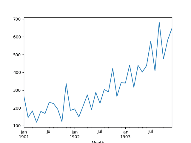
Line Plot of Shampoo Sales Dataset

Next, we will take a look at the LSTM configuration and test harness used in the experiment.

Experimental Test Harness

This section describes the test harness used in this tutorial.

Data Split

We will split the Shampoo Sales dataset into two parts: a training and a test set.

The first two years of data will be taken for the training dataset and the remaining one year of data will be used for the test set.

Models will be developed using the training dataset and will make predictions on the test dataset.

The persistence forecast (naive forecast) on the test dataset achieves an error of 136.761 monthly shampoo sales. This provides a lower acceptable bound of performance on the test set.

Model Evaluation

A rolling-forecast scenario will be used, also called walk-forward model validation.

Each time step of the test dataset will be walked one at a time. A model will be used to make a forecast for the time step, then the actual expected value from the test set will be taken and made available to the model for the forecast on the next time step.

This mimics a real-world scenario where new Shampoo Sales observations would be available each month and used in the forecasting of the following month.

This will be simulated by the structure of the train and test datasets.

All forecasts on the test dataset will be collected and an error score calculated to summarize the skill of the model. The root mean squared error (RMSE) will be used as it punishes large errors and results in a score that is in the same units as the forecast data, namely monthly shampoo sales.

Data Preparation

Before we can fit an LSTM model to the dataset, we must transform the data.

The following three data transforms are performed on the dataset prior to fitting a model and making a forecast.

Transform the time series data so that it is stationary. Specifically a lag=1 differencing to remove the increasing trend in the data.
Transform the time series into a supervised learning problem. Specifically the organization of data into input and output patterns where the observation at the previous time step is used as an input to forecast the observation at the current time step
Transform the observations to have a specific scale. Specifically, to rescale the data to values between -1 and 1 to meet the default hyperbolic tangent activation function of the LSTM model.

These transforms are inverted on forecasts to return them into their original scale before calculating and error score.

LSTM Model

We will use a base stateful LSTM model with 1 neuron fit for 1000 epochs.

A batch size of 1 is required as we will be using walk-forward validation and making one-step forecasts for each of the final 12 months of test data.

A batch size of 1 means that the model will be fit using online training (as opposed to batch training or mini-batch training). As a result, it is expected that the model fit will have some variance.

Ideally, more training epochs would be used (such as 1500), but this was truncated to 1000 to keep run times reasonable.

The model will be fit using the efficient ADAM optimization algorithm and the mean squared error loss function.

Experimental Runs

Each experimental scenario will be run 100 times and the RMSE score on the test set will be recorded from the end each run.

All test RMSE scores are written to file for later analysis.

Let’s dive into the experiments.

Code and Collect Results

The complete code listing is provided below.

It may take a few hours to run on modern hardware.

from pandas import DataFrame
from pandas import Series
from pandas import concat
from pandas import read_csv
from pandas import datetime
from sklearn.metrics import mean_squared_error
from sklearn.preprocessing import MinMaxScaler
from keras.models import Sequential
from keras.layers import Dense
from keras.layers import LSTM
from math import sqrt
import matplotlib
import numpy
from numpy import concatenate

# date-time parsing function for loading the dataset
def parser(x):
	return datetime.strptime('190'+x, '%Y-%m')

# frame a sequence as a supervised learning problem
def timeseries_to_supervised(data, lag=1):
	df = DataFrame(data)
	columns = [df.shift(i) for i in range(1, lag+1)]
	columns.append(df)
	df = concat(columns, axis=1)
	return df

# create a differenced series
def difference(dataset, interval=1):
	diff = list()
	for i in range(interval, len(dataset)):
		value = dataset[i] - dataset[i - interval]
		diff.append(value)
	return Series(diff)

# invert differenced value
def inverse_difference(history, yhat, interval=1):
	return yhat + history[-interval]

# scale train and test data to [-1, 1]
def scale(train, test):
	# fit scaler
	scaler = MinMaxScaler(feature_range=(-1, 1))
	scaler = scaler.fit(train)
	# transform train
	train = train.reshape(train.shape[0], train.shape[1])
	train_scaled = scaler.transform(train)
	# transform test
	test = test.reshape(test.shape[0], test.shape[1])
	test_scaled = scaler.transform(test)
	return scaler, train_scaled, test_scaled

# inverse scaling for a forecasted value
def invert_scale(scaler, X, yhat):
	new_row = [x for x in X] + [yhat]
	array = numpy.array(new_row)
	array = array.reshape(1, len(array))
	inverted = scaler.inverse_transform(array)
	return inverted[0, -1]

# fit an LSTM network to training data
def fit_lstm(train, batch_size, nb_epoch, neurons):
	X, y = train[:, 0:-1], train[:, -1]
	X = X.reshape(X.shape[0], 1, X.shape[1])
	model = Sequential()
	model.add(LSTM(neurons, batch_input_shape=(batch_size, X.shape[1], X.shape[2]), stateful=True))
	model.add(Dense(1))
	model.compile(loss='mean_squared_error', optimizer='adam')
	for i in range(nb_epoch):
		model.fit(X, y, epochs=1, batch_size=batch_size, verbose=0, shuffle=False)
		model.reset_states()
	return model

# make a one-step forecast
def forecast_lstm(model, batch_size, X):
	X = X.reshape(1, 1, len(X))
	yhat = model.predict(X, batch_size=batch_size)
	return yhat[0,0]

# run a repeated experiment
def experiment(repeats, series):
	# transform data to be stationary
	raw_values = series.values
	diff_values = difference(raw_values, 1)
	# transform data to be supervised learning
	supervised = timeseries_to_supervised(diff_values, 1)
	supervised_values = supervised.values[1:,:]
	# split data into train and test-sets
	train, test = supervised_values[0:-12, :], supervised_values[-12:, :]
	# transform the scale of the data
	scaler, train_scaled, test_scaled = scale(train, test)
	# run experiment
	error_scores = list()
	for r in range(repeats):
		# fit the base model
		lstm_model = fit_lstm(train_scaled, 1, 1000, 1)
		# forecast test dataset
		predictions = list()
		for i in range(len(test_scaled)):
			# predict
			X, y = test_scaled[i, 0:-1], test_scaled[i, -1]
			yhat = forecast_lstm(lstm_model, 1, X)
			# invert scaling
			yhat = invert_scale(scaler, X, yhat)
			# invert differencing
			yhat = inverse_difference(raw_values, yhat, len(test_scaled)+1-i)
			# store forecast
			predictions.append(yhat)
		# report performance
		rmse = sqrt(mean_squared_error(raw_values[-12:], predictions))
		print('%d) Test RMSE: %.3f' % (r+1, rmse))
		error_scores.append(rmse)
	return error_scores

# execute the experiment
def run():
	# load dataset
	series = read_csv('shampoo-sales.csv', header=0, parse_dates=[0], index_col=0, squeeze=True, date_parser=parser)
	# experiment
	repeats = 100
	results = DataFrame()
	# run experiment
	results['results'] = experiment(repeats, series)
	# summarize results
	print(results.describe())
	# save results
	results.to_csv('experiment_stateful.csv', index=False)

 # entry point
run()

100

101

102

103

104

105

106

107

108

109

110

111

112

113

114

115

116

117

118

119

120

121

122

123

124

125

126

127

128

129

130

from pandas import DataFrame

from pandas import Series

from pandas import concat

from pandas import read_csv

from pandas import datetime

from sklearn.metrics import mean_squared_error

from sklearn.preprocessing import MinMaxScaler

from keras.models import Sequential

from keras.layers import Dense

from keras.layers import LSTM

from math import sqrt

import matplotlib

import numpy

from numpy import concatenate

# date-time parsing function for loading the dataset

def parser(x):

return datetime.strptime('190'+x, '%Y-%m')

# frame a sequence as a supervised learning problem

def timeseries_to_supervised(data, lag=1):

df = DataFrame(data)

columns = [df.shift(i) for i in range(1, lag+1)]

columns.append(df)

df = concat(columns, axis=1)

return df

# create a differenced series

def difference(dataset, interval=1):

diff = list()

for i in range(interval, len(dataset)):

value = dataset[i] - dataset[i - interval]

diff.append(value)

return Series(diff)

# invert differenced value

def inverse_difference(history, yhat, interval=1):

return yhat + history[-interval]

# scale train and test data to [-1, 1]

def scale(train, test):

# fit scaler

scaler = MinMaxScaler(feature_range=(-1, 1))

scaler = scaler.fit(train)

# transform train

train = train.reshape(train.shape[0], train.shape[1])

train_scaled = scaler.transform(train)

# transform test

test = test.reshape(test.shape[0], test.shape[1])

test_scaled = scaler.transform(test)

return scaler, train_scaled, test_scaled

# inverse scaling for a forecasted value

def invert_scale(scaler, X, yhat):

new_row = [x for x in X] + [yhat]

array = numpy.array(new_row)

array = array.reshape(1, len(array))

inverted = scaler.inverse_transform(array)

return inverted[0, -1]

# fit an LSTM network to training data

def fit_lstm(train, batch_size, nb_epoch, neurons):

X, y = train[:, 0:-1], train[:, -1]

X = X.reshape(X.shape[0], 1, X.shape[1])

model = Sequential()

model.add(LSTM(neurons, batch_input_shape=(batch_size, X.shape[1], X.shape[2]), stateful=True))

model.add(Dense(1))

model.compile(loss='mean_squared_error', optimizer='adam')

for i in range(nb_epoch):

model.fit(X, y, epochs=1, batch_size=batch_size, verbose=0, shuffle=False)

model.reset_states()

return model

# make a one-step forecast

def forecast_lstm(model, batch_size, X):

X = X.reshape(1, 1, len(X))

yhat = model.predict(X, batch_size=batch_size)

return yhat[0,0]

# run a repeated experiment

def experiment(repeats, series):

# transform data to be stationary

raw_values = series.values

diff_values = difference(raw_values, 1)

# transform data to be supervised learning

supervised = timeseries_to_supervised(diff_values, 1)

supervised_values = supervised.values[1:,:]

# split data into train and test-sets

train, test = supervised_values[0:-12, :], supervised_values[-12:, :]

# transform the scale of the data

scaler, train_scaled, test_scaled = scale(train, test)

# run experiment

error_scores = list()

for r in range(repeats):

# fit the base model

lstm_model = fit_lstm(train_scaled, 1, 1000, 1)

# forecast test dataset

predictions = list()

for i in range(len(test_scaled)):

# predict

X, y = test_scaled[i, 0:-1], test_scaled[i, -1]

yhat = forecast_lstm(lstm_model, 1, X)

# invert scaling

yhat = invert_scale(scaler, X, yhat)

# invert differencing

yhat = inverse_difference(raw_values, yhat, len(test_scaled)+1-i)

# store forecast

predictions.append(yhat)

# report performance

rmse = sqrt(mean_squared_error(raw_values[-12:], predictions))

print('%d) Test RMSE: %.3f' % (r+1, rmse))

error_scores.append(rmse)

return error_scores

# execute the experiment

def run():

# load dataset

series = read_csv('shampoo-sales.csv', header=0, parse_dates=[0], index_col=0, squeeze=True, date_parser=parser)

# experiment

repeats = 100

results = DataFrame()

# run experiment

results['results'] = experiment(repeats, series)

# summarize results

print(results.describe())

# save results

results.to_csv('experiment_stateful.csv', index=False)

# entry point

run()

Running the experiment saves the RMSE scores of the fit model on the test dataset.

Results are saved to the file “experiment_stateful.csv“.

Note: Your results may vary given the stochastic nature of the algorithm or evaluation procedure, or differences in numerical precision. Consider running the example a few times and compare the average outcome.

A truncated listing of the results is provided below.

...
116.39769471284067
105.0459745537738
93.57827109861229
128.973001927212
97.02915084460737
198.56877142225886
113.09568645243242
97.84127724751188
124.60413895331735
111.62139008607713

...

116.39769471284067

105.0459745537738

93.57827109861229

128.973001927212

97.02915084460737

198.56877142225886

113.09568645243242

97.84127724751188

124.60413895331735

111.62139008607713

Basic Statistics on Results

We can start off by calculating some basic statistics on the entire population of 100 test RMSE scores.

Generally, we expect machine learning results to have a Gaussian distribution. This allows us to report the mean and standard deviation of a model and indicate a confidence interval for the model when making predictions on unseen data.

The snippet below loads the result file and calculates some descriptive statistics.

from pandas import DataFrame
from pandas import read_csv
from numpy import mean
from numpy import std
from matplotlib import pyplot
# load results file
results = read_csv('experiment_stateful.csv', header=0)
# descriptive stats
print(results.describe())
# box and whisker plot
results.boxplot()
pyplot.show()

from pandas import DataFrame

from pandas import read_csv

from numpy import mean

from numpy import std

from matplotlib import pyplot

# load results file

results = read_csv('experiment_stateful.csv', header=0)

# descriptive stats

print(results.describe())

# box and whisker plot

results.boxplot()

pyplot.show()

Running the example prints descriptive statistics from the results.

We can see that on average, the configuration achieved an RMSE of about 107 monthly shampoo sales with a standard deviation of about 17.

We can also see that the best test RMSE observed was about 90 sales, whereas the worse was just under 200, which is quite a spread of scores.

          results
count  100.000000
mean   107.051146
std     17.694512
min     90.407323
25%     96.630800
50%    102.603908
75%    111.199574
max    198.568771

results

count 100.000000

mean 107.051146

std 17.694512

min 90.407323

25% 96.630800

50% 102.603908

75% 111.199574

max 198.568771

To get a better idea of the spread of the data, a box and whisker plot is also created.

The plot shows the median (green line), middle 50% of the data (box), and outliers (dots). We can see quite a spread to the data towards poor RMSE scores.

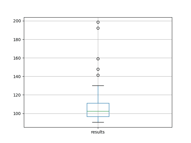
Box and Whisker Plot of 100 Test RMSE Scores on the Shampoo Sales Dataset

A histogram of the raw result values is also created.

The plot suggests a skewed or even an exponential distribution with a mass around an RMSE of 100 and a long tail leading out towards an RMSE of 200.

The distribution of the results are clearly not Gaussian. This is unfortunate, as the mean and standard deviation cannot be used directly to estimate a confidence interval for the model (e.g. 95% confidence as 2x the standard deviation around the mean).

The skewed distribution also highlights that the median (50th percentile) would be a better central tendency to use instead of the mean for these results. The median should be more robust to outlier results than the mean.

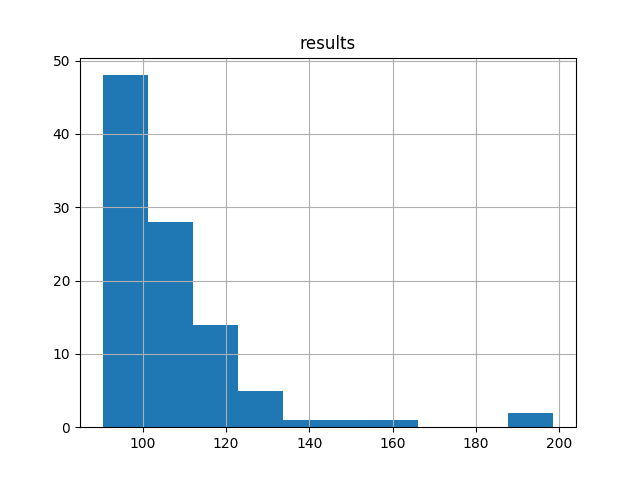
Histogram of Test RMSE Scores on Shampoo Sales Dataset

Repeats vs Test RMSE

We can start to look at how the summary statistics for the experiment change as the number of repeats is increased from 1 to 100.

We can accumulate the test RMSE scores and calculate descriptive statistics. For example, the score from one repeat, the scores from the first and second repeats, the scores from the first 3 repeats, and so on to 100 repeats.

We can review how the central tendency changes as the number of repeats is increased as a line plot. We’ll look at both the mean and median.

Generally, we would expect that as the number of repeats of the experiment is increased, the distribution would increasingly better match the underlying distribution, including the central tendency, such as the mean.

The complete code listing is provided below.

from pandas import DataFrame
from pandas import read_csv
from numpy import median
from numpy import mean
from matplotlib import pyplot
import numpy
# load results file
results = read_csv('experiment_stateful.csv', header=0)
values = results.values
# collect cumulative stats
medians, means = list(), list()
for i in range(1,len(values)+1):
	data = values[0:i, 0]
	mean_rmse, median_rmse = mean(data), median(data)
	means.append(mean_rmse)
	medians.append(median_rmse)
	print(i, mean_rmse, median_rmse)
# line plot of cumulative values
line1, = pyplot.plot(medians, label='Median RMSE')
line2, = pyplot.plot(means, label='Mean RMSE')
pyplot.legend(handles=[line1, line2])
pyplot.show()

from pandas import DataFrame

from pandas import read_csv

from numpy import median

from numpy import mean

from matplotlib import pyplot

import numpy

# load results file

results = read_csv('experiment_stateful.csv', header=0)

values = results.values

# collect cumulative stats

medians, means = list(), list()

for i in range(1,len(values)+1):

data = values[0:i, 0]

mean_rmse, median_rmse = mean(data), median(data)

means.append(mean_rmse)

medians.append(median_rmse)

print(i, mean_rmse, median_rmse)

# line plot of cumulative values

line1, = pyplot.plot(medians, label='Median RMSE')

line2, = pyplot.plot(means, label='Mean RMSE')

pyplot.legend(handles=[line1, line2])

pyplot.show()

The cumulative size of the distribution, mean, and median is printed as the number of repeats is increased.

A truncated output is listed below.

...
90 105.759546832 101.477640071
91 105.876449555 102.384620485
92 105.867422653 102.458057114
93 105.735281239 102.384620485
94 105.982491033 102.458057114
95 105.888245347 102.384620485
96 106.853667494 102.458057114
97 106.918018205 102.531493742
98 106.825398399 102.458057114
99 107.004981637 102.531493742
100 107.051145721 102.603907965

...

90 105.759546832 101.477640071

91 105.876449555 102.384620485

92 105.867422653 102.458057114

93 105.735281239 102.384620485

94 105.982491033 102.458057114

95 105.888245347 102.384620485

96 106.853667494 102.458057114

97 106.918018205 102.531493742

98 106.825398399 102.458057114

99 107.004981637 102.531493742

100 107.051145721 102.603907965

A line plot is also created showing how the mean and median change as the number of repeats is increased.

The results show that the mean is more influenced by outlier results than the median, as expected.

We can see that the median appears quite stable down around 99-100. This jumps to 102 towards the end of the plot suggesting a string of worse RMSE scores at later repeats.

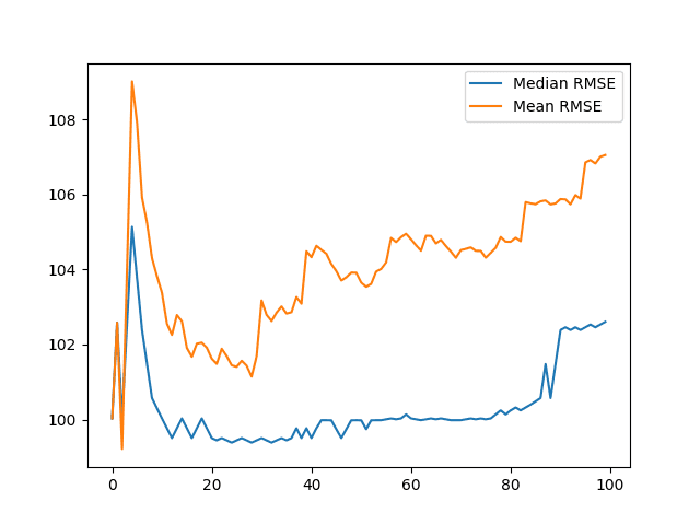
Line Plots of Mean and Median Test RMSE vs Number of Repeats

Review of Results

We made some useful observations from 100 repeats of a stateful LSTM on a standard time series forecasting problem.

Specifically:

We observed that the distribution of results is not Gaussian. It may be a skewed Gaussian or an exponential distribution with a long tail and outliers.
We observed that the distribution of results did not stabilize with the increase of repeats from 1 to 100.

The observations suggest a few important properties:

The choice of online learning for the LSTM and problem results in a relatively unstable model.
The chosen number of repeats (100) may not be sufficient to characterize the behavior of the model.

This is a useful finding as it would be a mistake to make strong conclusions about the model from 100 or fewer repeats of the experiment.

This is an important caution to consider when describing your own machine learning results.

This suggests some extensions to this experiment, such as:

Explore the impact of the number of repeats on a more stable model, such as one using batch or mini-batch learning.
Increase the number of repeats to thousands or more in an attempt to account for the general instability of the model with online learning.

Summary

In this tutorial, you discovered how to analyze experimental results from LSTM models fit using online learning.

You learned:

How to design a robust test harness for evaluating LSTM models on time series forecast problems.
How to analyze experimental results, including summary statistics.
How to analyze the impact of increasing the number of experiment repeats and how to identify an unstable model.

Do you have any questions?
Ask your questions in the comments below and I will do my best to answer.

33 Responses to Instability of Online Learning for Stateful LSTM for Time Series Forecasting

Cao May 31, 2017 at 8:48 pm #

Dear Jason,

always thank you for your posts, which are really helpful.

i am a beginner of machine learning, and i stuck in some questions for a longtime.

1.what is the online learning? batch size=1 is online and dynamic?

2.how to set a lstm structure, which can dynamic add new data every minutes, and update the weight and bias or something else. then it can predict every next minute data.

thank you again, jason.

Reply
- Jason Brownlee June 2, 2017 at 12:47 pm #
  
  Online learning means the model is updated after each training pattern.
  
  The structure does not change. You need to find a structure that achieves good results on your problem.
  
  Reply
Norman March 16, 2018 at 7:00 am #

Dear Jason,

thank you for sharing your knowledge!
Is your LSTM stateful?
To my mind you have to set stateful=True in line 66 or does this happen automatically with batchsize=1?

Best regards

Reply
- Norman March 16, 2018 at 8:09 am #
  
  I’m sorry I didn’t see the stateful=True
  
  Reply
- Jason Brownlee March 16, 2018 at 2:22 pm #
  
  Yes, it means that state is only reset when done so explicitly.
  
  Reply
Mathias A March 24, 2018 at 2:16 am #

I have seen you use this structure a lot:

for i in range(nb_epoch):
model.fit(X, y, epochs=1, batch_size=batch_size, verbose=0, shuffle=False)
model.reset_states()

I found out that callbacks in keras can be used instead of wrapping fit() in a loop:

# define callback class
class ModelStateReset(keras.callbacks.Callback):
def on_epoch_end(self, epoch, logs={}):
self.model.reset_states()
reset = ModelStateReset()

# use reset callback instance in fit
model.fit(x, y, epochs=i, batch_size=batch_size, shuffle=False, callbacks=[reset])

Just a heads up if you missed this. I personally prefer using fit()’s own parameters over the loop 😉

Reply
- Jason Brownlee March 24, 2018 at 6:30 am #
  
  Thanks for sharing.
  
  Reply
Carlos B April 8, 2018 at 12:11 am #

Thank you for this post, Jason. You have cleared up my confusion regarding the results from my initial LSTM tests for my research. Are all LSTMs stochastic by nature, because of the random weights initialisation?

Reply
- Jason Brownlee April 8, 2018 at 6:21 am #
  
  Yes, see this post:
  https://machinelearningmastery.com/randomness-in-machine-learning/
  
  Reply
Harsh June 28, 2018 at 12:05 am #

HI Jason,
Thanks for your wonderful posts!

I am working with time series data and am using lstms for that. I am doing online learning(batch_size=1) with stateful lstms for a univariate series and considering timesteps=200.

This is how the training is being done:

for i in range(NUM_EPOCHS):
print(“Epoch {:d}/{:d}”.format(i+1, NUM_EPOCHS))
model.fit(Xtrain, Ytrain, batch_size=BATCH_SIZE, epochs=1, verbose =1, callbacks=callbacks_list, shuffle=False)
model.reset_states()

where callbacks list is just for early stopping and reducing LR on plateau.

And for predicting:

predictions = model.predict(Xtest,batch_size=BATCH_SIZE)

Since I am doing online learning, so when the new data comes (lets say every hour), I don’t want to retrain the model from scratch. The idea would be to just update the trained model with new data and do the prediction for the new data. So, do I just save the weights after fitting the training data and load the saved weights before predicting? Would that be enough? Will it also save the state as I am using a stateful lstm? Could you please tell me if I am thinking it in the right way or suggest something else?

Reply
- Jason Brownlee June 28, 2018 at 6:22 am #
  
  Yes, you can update the weights with new data.
  
  Generally, I would encourage you to try other methods as I have found LSTMs to be very poor at time series forecasting compared to other methods.
  
  Reply
  - Anas July 11, 2018 at 11:24 pm #
    
    Hi Jason,
    Thank you for your post.
    Could you suggest me some of these methods for time series forecasting?
    
    Reply
    - Jason Brownlee July 12, 2018 at 6:26 am #
      
      Yes, try a suite of classical methods (SARIMA, ETC, etc.), a suite of ML methods (linear and nonlinear) and a suite of deep learning methods (mlp, cnn, lstm, etc.)
      
      Reply
      - Anas July 13, 2018 at 5:25 pm #
        
        Thank you Jason for your answer.
- Narendran Raghavan April 10, 2019 at 4:17 am #
  
  Hi Harsh, I am doing a similar problem as yours in online time series forecasting using LSTMs. I wanted your input and help in my problem. Is there a good way to contact you? Thanks, Narendran
  
  Reply
Harsh June 28, 2018 at 10:17 pm #

I already implemented ARIMA but it’s too slow as it needs to be retrained everytime new data comes in. And finding the values of p and q using grid search consumes a lot of time.

That’s why I switched to stateful LSTMs and surprisingly I am getting better results with LSTM and is faster as well.

I have few more questions:

1. I am getting different predictions everytime I run the model. Do you know how can we get consistent results everytime? I saw you have used repeats and taking the average for rmse but I want to know if there is a way to get the same predictions.

2. Once I save the model weights after fitting the training data and load the weights before predicting, would it also load the state that existed when we saved the weights? Do you have an example where you are doing more than a basic LSTM example e.g. how one would implement in a real time scenario(end-to-end model).

Reply
- Jason Brownlee June 29, 2018 at 6:08 am #
  
  Glad to hear it.
  
  Yes, this is a feature of neural networks, you can learn more here:
  https://machinelearningmastery.com/randomness-in-machine-learning/
  
  If state is critical, you can use a warm start by predicting on training data first before predicting on new data, and not resetting state in-between. I would be surprised if state matters that much though.
  
  Reply
  - Jack September 18, 2018 at 8:00 am #
    
    Cant you also use random_seed to make your model deterministic?
    
    Reply
    - Jason Brownlee September 18, 2018 at 2:17 pm #
      
      Not quite:
      https://machinelearningmastery.com/reproducible-results-neural-networks-keras/
      
      Reply
Gabriel Mouzella Silva September 30, 2018 at 5:28 am #

Hi Jason,

could an already trained stable network be retrained online and still be stable? once the weights will not be random, and it would be something like doing a transfer learning.

I ask that because i’m working with an already trained LSTM, however i’m facing the concept drift problem and i’m forced to retrain my model every now and then so the forecast remains good enough for my aplication

Reply
- Jason Brownlee September 30, 2018 at 6:09 am #
  
  It can, perhaps try mix in some older samples as well.
  
  I have more on the topic here:
  https://machinelearningmastery.com/gentle-introduction-concept-drift-machine-learning/
  
  Reply
  - Gabriel Mouzella Silva October 2, 2018 at 11:59 am #
    
    Thanks
    
    Reply
Sus November 19, 2018 at 8:00 am #

Hi Jason,

Thanks for the great tutorials.

Two questions:

– From the tutorial I assume a solution for this problem is increasing the batch size? Do you have any tutorial from a stateful LSTM network using batch size > 1?-

– Is it possible using the early stopping callback here?

– How about transforming the data to Gaussian (as mentioned here: https://machinelearningmastery.com/how-to-transform-data-to-fit-the-normal-distribution/)?

Thanks in advance!!!

Reply
- Jason Brownlee November 19, 2018 at 2:19 pm #
  
  Yes, I have more examples of LSTMs with managed state and larger batch sizes. Perhaps start here:
  https://machinelearningmastery.com/start-here/#lstm
  
  Early stopping would have to be manual if the epochs are walked manually.
  
  You can transform the data.
  
  Reply
  - Sus November 19, 2018 at 8:05 pm #
    
    Great! Thanks for your prompt reply!
    
    Reply
Mitchel Offiong September 14, 2019 at 12:35 am #

Hello Brownlee,

Thank you for this heads up. I am interested in online training and prediction for real time time-series data.

If your book contains it, i will like to to have and possibly a step by step guy as i am relatively new to the weight update concept of real time prediction. Thanks

Reply
- Jason Brownlee September 14, 2019 at 6:20 am #
  
  What do you mean by real time?
  
  Do you mean refitting a model after each new observation?
  
  Or do you mean simply making predictions as needed?
  
  Reply
  - James Bowery January 9, 2020 at 9:32 am #
    
    “Realtime” in the context of a blog post about “Online” means both predicting each new observation and refitting the model after each new observation.
    
    Reply
    - Jason Brownlee January 9, 2020 at 1:49 pm #
      
      I don’t really have much on updating models with new samples.
      
      Generally, it sounds straightforward, as long as you verify with controlled experiments that your chosen update schedule results in skillful models. No point in updating the model (weights) if it does not improve the performance.
      
      Reply
FrederikB February 7, 2020 at 3:14 am #

Hi Jason, been learning alot from your posts, thanx!!

On this topic: I have a few local weather sensors that I get data from every 10min, and I’d like to try and test what sort of outcome I can get from incremental learning on these new data coming in vs pre-trained model.

1 – What I’m thinking is appending the new data onto the big dataset and then using slice to sample a prediction set equal to my timesteps to make a prediction 1 step into the future only.(Chose 10min just because I’ll get more data regularly to test with) And then display that in the app.

2 – After the previous step I create a single train set: X[-60 :-1 , : ] and y[-1,0] from the main dataset (timeSteps = 60) that I fit to the model with Batch_size=1 to get the latest updates.

I’ll be using a stacked LSTM.

I’m busy designing /figuring out how to design it, but I’d like realistic feedback before I go to far, or if you have any suggestion how else to approach this?
Much appreciated.

Reply
- Jason Brownlee February 7, 2020 at 8:23 am #
  
  I recommend this framework to confirm the LSTM adds value over a linear model:
  https://machinelearningmastery.com/how-to-develop-a-skilful-time-series-forecasting-model/
  
  Reply
Andrey August 26, 2020 at 8:15 am #

Hi Jason, thanks for sharing this valuable information. I appreciate if you respond at my question. For my project i divided my data in train, validation and test sets. I wonder about what to do after select the structure that works better to my problem (i did this using the validation set), should i’ve re-train the model including train and validation data? or there’s a way to update the model including the validation data before prediction on test set?. This is on my mind because wheni re-train the model with the structure selected, i feel that the new data affect the results that i obtained before,

Thanks a lot for your blog, it was very helpfull for the purpose of my project.

Regards!

Reply
- Jason Brownlee August 26, 2020 at 1:43 pm #
  
  You’re welcome.
  
  Good question, ideally you want to train a final model with all available data if you can.
  
  Reply

Navigation

Instability of Online Learning for Stateful LSTM for Time Series Forecasting

Model Instability

Tutorial Overview

Environment

Need help with Deep Learning for Time Series?

Shampoo Sales Dataset

Experimental Test Harness

Data Split

Model Evaluation

Data Preparation

LSTM Model

Experimental Runs

Code and Collect Results

Basic Statistics on Results

Repeats vs Test RMSE

Review of Results

Summary

Develop Deep Learning models for Time Series Today!

Develop Your Own Forecasting models in Minutes

Finally Bring Deep Learning to your Time Series Forecasting Projects

More On This Topic

33 Responses to Instability of Online Learning for Stateful LSTM for Time Series Forecasting

Leave a Reply Click here to cancel reply.