Configuring neural networks is difficult because there is no good theory on how to do it.
You must be systematic and explore different configurations both from a dynamical and an objective results point of a view to try to understand what is going on for a given predictive modeling problem.
In this tutorial, you will discover how you can explore how to configure an LSTM network on a time series forecasting problem.
After completing this tutorial, you will know:
How to tune and interpret the results of the number of training epochs.
How to tune and interpret the results of the size of training batches.
How to tune and interpret the results of the number of neurons.
Kick-start your project with my new book Deep Learning for Time Series Forecasting, including step-by-step tutorials and the Python source code files for all examples.
Let’s get started.
Updated Apr/2019: Updated the link to dataset.
How to Tune LSTM Hyperparameters with Keras for Time Series Forecasting Photo by David Saddler, some rights reserved.
Tutorial Overview
This tutorial is broken down into 6 parts; they are:
Shampoo Sales Dataset
Experimental Test Harness
Tuning the Number of Epochs
Tuning the Batch Size
Tuning the Number of Neurons
Summary of Results
Environment
This tutorial assumes you have a Python SciPy environment installed. You can use either Python 2 or 3 with this example.
This tutorial assumes you have Keras v2.0 or higher installed with either the TensorFlow or Theano backend.
The tutorial also assumes you have scikit-learn, Pandas, NumPy and Matplotlib installed.
If you need help setting up your Python environment, see this post:
Running the example loads the dataset as a Pandas Series and prints the first 5 rows.
1
2
3
4
5
6
7
Month
1901-01-01 266.0
1901-02-01 145.9
1901-03-01 183.1
1901-04-01 119.3
1901-05-01 180.3
Name: Sales, dtype: float64
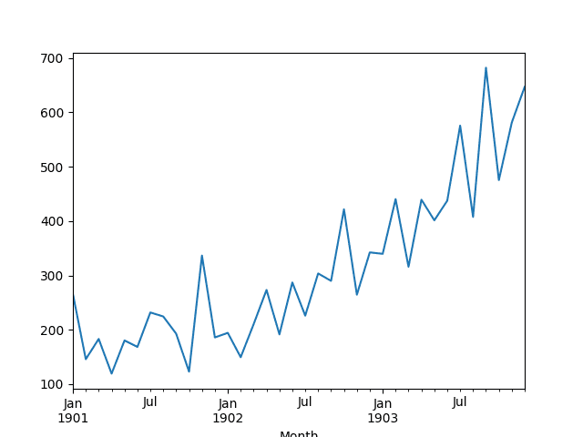
A line plot of the series is then created showing a clear increasing trend.
Line Plot of Shampoo Sales Dataset
Next, we will take a look at the LSTM configuration and test harness used in the experiment.
Need help with Deep Learning for Time Series?
Take my free 7-day email crash course now (with sample code).
Click to sign-up and also get a free PDF Ebook version of the course.
Experimental Test Harness
This section describes the test harness used in this tutorial.
Data Split
We will split the Shampoo Sales dataset into two parts: a training and a test set.
The first two years of data will be taken for the training dataset and the remaining one year of data will be used for the test set.
Models will be developed using the training dataset and will make predictions on the test dataset.
The persistence forecast (naive forecast) on the test dataset achieves an error of 136.761 monthly shampoo sales. This provides a lower acceptable bound of performance on the test set.
Model Evaluation
A rolling-forecast scenario will be used, also called walk-forward model validation.
Each time step of the test dataset will be walked one at a time. A model will be used to make a forecast for the time step, then the actual expected value from the test set will be taken and made available to the model for the forecast on the next time step.
This mimics a real-world scenario where new Shampoo Sales observations would be available each month and used in the forecasting of the following month.
This will be simulated by the structure of the train and test datasets. We will make all of the forecasts in a one-shot method.
All forecasts on the test dataset will be collected and an error score calculated to summarize the skill of the model. The root mean squared error (RMSE) will be used as it punishes large errors and results in a score that is in the same units as the forecast data, namely monthly shampoo sales.
Data Preparation
Before we can fit an LSTM model to the dataset, we must transform the data.
The following three data transforms are performed on the dataset prior to fitting a model and making a forecast.
Transform the time series data so that it is stationary. Specifically, a lag=1 differencing to remove the increasing trend in the data.
Transform the time series into a supervised learning problem. Specifically, the organization of data into input and output patterns where the observation at the previous time step is used as an input to forecast the observation at the current time time step
Transform the observations to have a specific scale. Specifically, to rescale the data to values between -1 and 1 to meet the default hyperbolic tangent activation function of the LSTM model.
These transforms are inverted on forecasts to return them into their original scale before calculating and error score.
Experimental Runs
Each experimental scenario will be run 10 times.
The reason for this is that the random initial conditions for an LSTM network can result in very different results each time a given configuration is trained.
A diagnostic approach will be used to investigate model configurations. This is where line plots of model skill over time (training iterations called epochs) will be created and studied for insight into how a given configuration performs and how it may be adjusted to elicit better performance.
The model will be evaluated on both the train and the test datasets at the end of each epoch and the RMSE scores saved.
The train and test RMSE scores at the end of each scenario are printed to give an indication of progress.
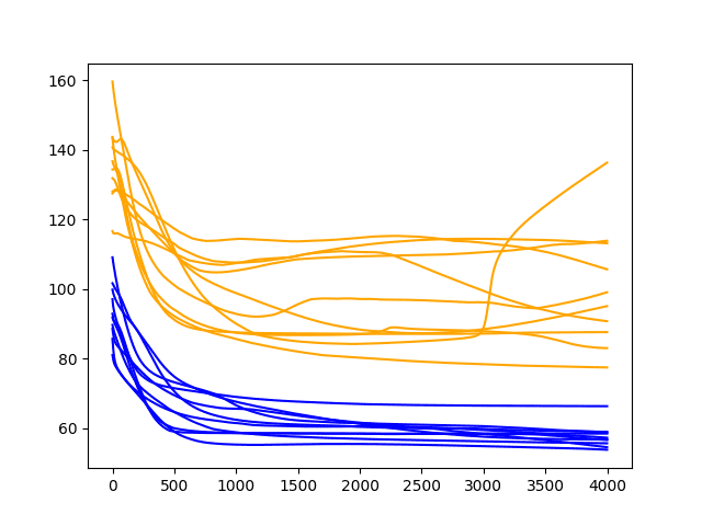
The series of train and test RMSE scores are plotted at the end of a run as a line plot. Train scores are colored blue and test scores are colored orange.
Let’s dive into the results.
Tuning the Number of Epochs
The first LSTM parameter we will look at tuning is the number of training epochs.
The model will use a batch size of 4, and a single neuron. We will explore the effect of training this configuration for different numbers of training epochs.
Diagnostic of 500 Epochs
The complete code listing for this diagnostic is listed below.
The code is reasonably well commented and should be easy to follow. This code will be the basis for all future experiments in this tutorial and only the changes made in each subsequent experiment will be listed.
1
2
3
4
5
6
7
8
9
10
11
12
13
14
15
16
17
18
19
20
21
22
23
24
25
26
27
28
29
30
31
32
33
34
35
36
37
38
39
40
41
42
43
44
45
46
47
48
49
50
51
52
53
54
55
56
57
58
59
60
61
62
63
64
65
66
67
68
69
70
71
72
73
74
75
76
77
78
79
80
81
82
83
84
85
86
87
88
89
90
91
92
93
94
95
96
97
98
99
100
101
102
103
104
105
106
107
108
109
110
111
112
113
114
115
116
117
118
119
120
121
122
123
124
125
126
127
128
129
130
131
132
133
134
135
136
137
138
from pandas import DataFrame
from pandas import Series
from pandas import concat
from pandas import read_csv
from pandas import datetime
from sklearn.metrics import mean_squared_error
from sklearn.preprocessing import MinMaxScaler
from keras.models import Sequential
from keras.layers import Dense
from keras.layers import LSTM
from math import sqrt
import matplotlib
# be able to save images on server
matplotlib.use('Agg')
from matplotlib import pyplot
import numpy
# date-time parsing function for loading the dataset
def parser(x):
returndatetime.strptime('190'+x,'%Y-%m')
# frame a sequence as a supervised learning problem
Note: Your results may vary given the stochastic nature of the algorithm or evaluation procedure, or differences in numerical precision. Consider running the example a few times and compare the average outcome.
Running the experiment prints the RMSE for the train and the test sets at the end of each of the 10 experimental runs.
1
2
3
4
5
6
7
8
9
10
0) TrainRMSE=63.495594, TestRMSE=113.472643
1) TrainRMSE=60.446307, TestRMSE=100.147470
2) TrainRMSE=59.879681, TestRMSE=95.112331
3) TrainRMSE=66.115269, TestRMSE=106.444401
4) TrainRMSE=61.878702, TestRMSE=86.572920
5) TrainRMSE=73.519382, TestRMSE=103.551694
6) TrainRMSE=64.407033, TestRMSE=98.849227
7) TrainRMSE=72.684834, TestRMSE=98.499976
8) TrainRMSE=77.593773, TestRMSE=124.404747
9) TrainRMSE=71.749335, TestRMSE=126.396615
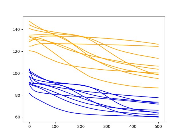
A line plot of the series of RMSE scores on the train and test sets after each training epoch is also created.
Diagnostic Results with 500 Epochs
The results clearly show a downward trend in RMSE over the training epochs for almost all of the experimental runs.
This is a good sign, as it shows the model is learning the problem and has some predictive skill. In fact, all of the final test scores are below the error of a simple persistence model (naive forecast) that achieves an RMSE of 136.761 on this problem.
The results suggest that more training epochs will result in a more skillful model.
Let’s try doubling the number of epochs from 500 to 1000.
Diagnostic of 1000 Epochs
In this section, we use the same experimental setup and fit the model over 1000 training epochs.
Specifically, the n_epochs parameter is set to 1000 in the run() function.
1
n_epochs=1000
Note: Your results may vary given the stochastic nature of the algorithm or evaluation procedure, or differences in numerical precision. Consider running the example a few times and compare the average outcome.
Running the example prints the RMSE for the train and test sets from the final epoch.
1
2
3
4
5
6
7
8
9
10
0) TrainRMSE=69.242394, TestRMSE=90.832025
1) TrainRMSE=65.445810, TestRMSE=113.013681
2) TrainRMSE=57.949335, TestRMSE=103.727228
3) TrainRMSE=61.808586, TestRMSE=89.071392
4) TrainRMSE=68.127167, TestRMSE=88.122807
5) TrainRMSE=61.030678, TestRMSE=93.526607
6) TrainRMSE=61.144466, TestRMSE=97.963895
7) TrainRMSE=59.922150, TestRMSE=94.291120
8) TrainRMSE=60.170052, TestRMSE=90.076229
9) TrainRMSE=62.232470, TestRMSE=98.174839
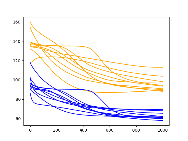
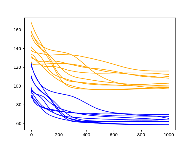
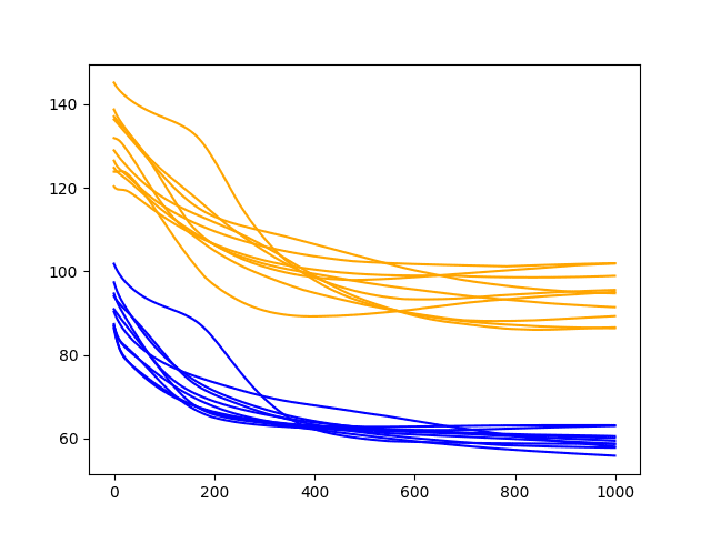
A line plot of the test and train RMSE scores each epoch is also created.
Diagnostic Results with 1000 Epochs
We can see that the downward trend of model error does continue and appears to slow.
The lines for the train and test cases become more horizontal, but still generally show a downward trend, although at a lower rate of change. Some examples of test error show a possible inflection point around 600 epochs and may show a rising trend.
It is worth extending the epochs further. We are interested in the average performance continuing to improve on the test set and this may continue.
Let’s try doubling the number of epochs from 1000 to 2000.
Diagnostic of 2000 Epochs
In this section, we use the same experimental setup and fit the model over 2000 training epochs.
Specifically, the n_epochs parameter is set to 2000 in the run() function.
1
n_epochs=2000
Note: Your results may vary given the stochastic nature of the algorithm or evaluation procedure, or differences in numerical precision. Consider running the example a few times and compare the average outcome.
Running the example prints the RMSE for the train and test sets from the final epoch.
1
2
3
4
5
6
7
8
9
10
0) TrainRMSE=67.292970, TestRMSE=83.096856
1) TrainRMSE=55.098951, TestRMSE=104.211509
2) TrainRMSE=69.237206, TestRMSE=117.392007
3) TrainRMSE=61.319941, TestRMSE=115.868142
4) TrainRMSE=60.147575, TestRMSE=87.793270
5) TrainRMSE=59.424241, TestRMSE=99.000790
6) TrainRMSE=66.990082, TestRMSE=80.490660
7) TrainRMSE=56.467012, TestRMSE=97.799062
8) TrainRMSE=60.386380, TestRMSE=103.810569
9) TrainRMSE=58.250862, TestRMSE=86.212094
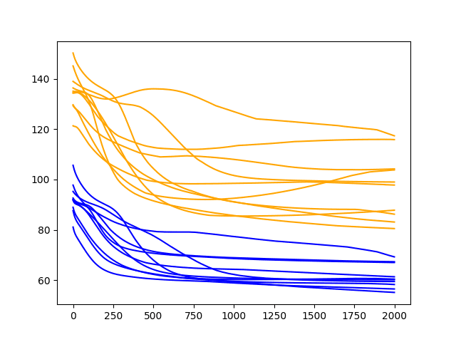
A line plot of the test and train RMSE scores each epoch is also created.
Diagnostic Results with 2000 Epochs
As one might have guessed, the downward trend in error continues over the additional 1000 epochs on both the train and test datasets.
Of note, about half of the cases continue to decrease in error all the way to the end of the run, whereas the rest show signs of an increasing trend.
The increasing trend is a sign of overfitting. This is when the model overfits the training dataset at the cost of worse performance on the test dataset. It is exemplified by continued improvements on the training dataset and improvements followed by an inflection point and worsting skill in the test dataset. A little less than half of the runs show the beginnings of this type of pattern on the test dataset.
Nevertheless, the final epoch results on the test dataset are very good. If there is a chance we can see further gains by even longer training, we must explore it.
Let’s try doubling the number of epochs from 2000 to 4000.
Diagnostic of 4000 Epochs
In this section, we use the same experimental setup and fit the model over 4000 training epochs.
Specifically, the n_epochs parameter is set to 4000 in the run() function.
1
n_epochs=4000
Note: Your results may vary given the stochastic nature of the algorithm or evaluation procedure, or differences in numerical precision. Consider running the example a few times and compare the average outcome.
Running the example prints the RMSE for the train and test sets from the final epoch.
1
2
3
4
5
6
7
8
9
10
0) TrainRMSE=58.889277, TestRMSE=99.121765
1) TrainRMSE=56.839065, TestRMSE=95.144846
2) TrainRMSE=58.522271, TestRMSE=87.671309
3) TrainRMSE=53.873962, TestRMSE=113.920076
4) TrainRMSE=66.386299, TestRMSE=77.523432
5) TrainRMSE=58.996230, TestRMSE=136.367014
6) TrainRMSE=55.725800, TestRMSE=113.206607
7) TrainRMSE=57.334604, TestRMSE=90.814642
8) TrainRMSE=54.593069, TestRMSE=105.724825
9) TrainRMSE=56.678498, TestRMSE=83.082262
A line plot of the test and train RMSE scores each epoch is also created.
Diagnostic Results with 4000 Epochs
A similar pattern continues.
There is a general trend of improving performance, even over the 4000 epochs. There is one case of severe overfitting where test error rises sharply.
Again, most runs end with a “good” (better than persistence) final test error.
Summary of Results
The diagnostic runs above are helpful to explore the dynamical behavior of the model, but fall short of an objective and comparable mean performance.
We can address this by repeating the same experiments and calculating and comparing summary statistics for each configuration. In this case, 30 runs were completed of the epoch values 500, 1000, 2000, 4000, and 6000.
The idea is to compare the configurations using summary statistics over a larger number of runs and see exactly which of the configurations might perform better on average.
The complete code example is listed below.
1
2
3
4
5
6
7
8
9
10
11
12
13
14
15
16
17
18
19
20
21
22
23
24
25
26
27
28
29
30
31
32
33
34
35
36
37
38
39
40
41
42
43
44
45
46
47
48
49
50
51
52
53
54
55
56
57
58
59
60
61
62
63
64
65
66
67
68
69
70
71
72
73
74
75
76
77
78
79
80
81
82
83
84
85
86
87
88
89
90
91
92
93
94
95
96
97
98
99
100
101
102
103
104
105
106
107
108
109
110
111
112
113
114
115
116
117
118
119
120
121
122
123
124
125
126
127
128
129
130
131
132
133
from pandas import DataFrame
from pandas import Series
from pandas import concat
from pandas import read_csv
from pandas import datetime
from sklearn.metrics import mean_squared_error
from sklearn.preprocessing import MinMaxScaler
from keras.models import Sequential
from keras.layers import Dense
from keras.layers import LSTM
from math import sqrt
import matplotlib
# be able to save images on server
matplotlib.use('Agg')
from matplotlib import pyplot
import numpy
# date-time parsing function for loading the dataset
def parser(x):
returndatetime.strptime('190'+x,'%Y-%m')
# frame a sequence as a supervised learning problem
Running the code first prints summary statistics for each of the 5 configurations. Notably, this includes the mean and standard deviations of the RMSE scores from each population of results.
Note: Your results may vary given the stochastic nature of the algorithm or evaluation procedure, or differences in numerical precision. Consider running the example a few times and compare the average outcome.
The mean gives an idea of the average expected performance of a configuration, whereas the standard deviation gives an idea of the variance. The min and max RMSE scores also give an idea of the range of possible best and worst case examples that might be expected.
Looking at just the mean RMSE scores, the results suggest that an epoch configured to 1000 may be better. The results also suggest further investigations may be warranted of epoch values between 1000 and 2000.
max 138.879278 139.928055 146.840997 157.026562 166.111151
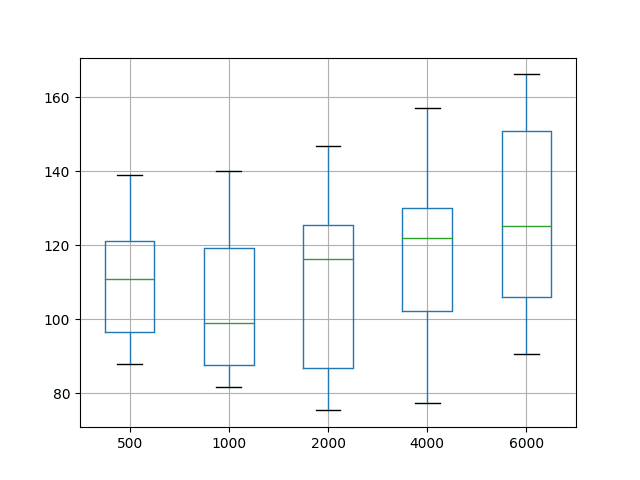
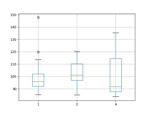
The distributions are also shown on a box and whisker plot. This is helpful to see how the distributions directly compare.
The green line shows the median and the box shows the 25th and 75th percentiles, or the middle 50% of the data. This comparison also shows that the choice of setting epochs to 1000 is better than the tested alternatives. It also shows that the best possible performance may be achieved with epochs of 2000 or 4000, at the cost of worse performance on average.
Box and Whisker Plot Summarizing Epoch Results
Next, we will look at the effect of batch size.
Tuning the Batch Size
Batch size controls how often to update the weights of the network.
Importantly in Keras, the batch size must be a factor of the size of the test and the training dataset.
In the previous section exploring the number of training epochs, the batch size was fixed at 4, which cleanly divides into the test dataset (with the size 12) and in a truncated version of the test dataset (with the size of 20).
In this section, we will explore the effect of varying the batch size. We will hold the number of training epochs constant at 1000.
Diagnostic of 1000 Epochs and Batch Size of 4
As a reminder, the previous section evaluated a batch size of 4 in the second experiment with a number of epochs of 1000.
The results showed a downward trend in error that continued for most runs all the way to the final training epoch.
Diagnostic Results with 1000 Epochs
Diagnostic of 1000 Epochs and Batch Size of 2
In this section, we look at halving the batch size from 4 to 2.
This change is made to the n_batch parameter in the run() function; for example:
1
n_batch=2
Running the example shows the same general trend in performance as a batch size of 4, perhaps with a higher RMSE on the final epoch.
Note: Your results may vary given the stochastic nature of the algorithm or evaluation procedure, or differences in numerical precision. Consider running the example a few times and compare the average outcome.
The runs may show the behavior of stabilizing the RMES sooner rather than seeming to continue the downward trend.
The RSME scores from the final exposure of each run are listed below.
1
2
3
4
5
6
7
8
9
10
0) TrainRMSE=63.510219, TestRMSE=115.855819
1) TrainRMSE=58.336003, TestRMSE=97.954374
2) TrainRMSE=69.163685, TestRMSE=96.721446
3) TrainRMSE=65.201764, TestRMSE=110.104828
4) TrainRMSE=62.146057, TestRMSE=112.153553
5) TrainRMSE=58.253952, TestRMSE=98.442715
6) TrainRMSE=67.306530, TestRMSE=108.132021
7) TrainRMSE=63.545292, TestRMSE=102.821356
8) TrainRMSE=61.693847, TestRMSE=99.859398
9) TrainRMSE=58.348250, TestRMSE=99.682159
A line plot of the test and train RMSE scores each epoch is also created.
Diagnostic Results with 1000 Epochs and Batch Size of 2
Let’s try having the batch size again.
Diagnostic of 1000 Epochs and Batch Size of 1
A batch size of 1 is technically performing online learning.
That is where the network is updated after each training pattern. This can be contrasted with batch learning, where the weights are only updated at the end of each epoch.
We can change the n_batch parameter in the run() function; for example:
1
n_batch=1
Note: Your results may vary given the stochastic nature of the algorithm or evaluation procedure, or differences in numerical precision. Consider running the example a few times and compare the average outcome.
Again, running the example prints the RMSE scores from the final epoch of each run.
1
2
3
4
5
6
7
8
9
10
0) TrainRMSE=60.349798, TestRMSE=100.182293
1) TrainRMSE=62.624106, TestRMSE=95.716070
2) TrainRMSE=64.091859, TestRMSE=98.598958
3) TrainRMSE=59.929993, TestRMSE=96.139427
4) TrainRMSE=59.890593, TestRMSE=94.173619
5) TrainRMSE=55.944968, TestRMSE=106.644275
6) TrainRMSE=60.570245, TestRMSE=99.981562
7) TrainRMSE=56.704995, TestRMSE=111.404182
8) TrainRMSE=59.909065, TestRMSE=90.238473
9) TrainRMSE=60.863807, TestRMSE=105.331214
A line plot of the test and train RMSE scores each epoch is also created.
The plot suggests more variability in the test RMSE over time and perhaps a train RMSE that stabilizes sooner than with larger batch sizes. The increased variability in the test RMSE is to be expected given the large changes made to the network give so little feedback each update.
The graph also suggests that perhaps the decreasing trend in RMSE may continue if the configuration was afforded more training epochs.
Diagnostic Results with 1000 Epochs and Batch Size of 1
Summary of Results
As with training epochs, we can objectively compare the performance of the network given different batch sizes.
Each configuration was run 30 times and summary statistics calculated on the final results.
Note: Your results may vary given the stochastic nature of the algorithm or evaluation procedure, or differences in numerical precision. Consider running the example a few times and compare the average outcome.
From the mean performance alone, the results suggest lower RMSE with a batch size of 1. As was noted in the previous section, this may be improved further with more training epochs.
1
2
3
4
5
6
7
8
9
1 2 4
count 30.000000 30.000000 30.000000
mean 98.697017 102.642594 100.320203
std 12.227885 9.144163 15.957767
min 85.172215 85.072441 83.636365
25% 92.023175 96.834628 87.671461
50% 95.981688 101.139527 91.628144
75% 102.009268 110.171802 114.660192
max 147.688818 120.038036 135.290829
A box and whisker plot of the data was also created to help graphically compare the distributions. The plot shows the median performance as a green line where a batch size of 4 shows both the largest variability and also the lowest median RMSE.
Tuning a neural network is a tradeoff of average performance and variability of that performance, with an ideal result having a low mean error with low variability, meaning that it is generally good and reproducible.
Box and Whisker Plot Summarizing Batch Size Results
Tuning the Number of Neurons
In this section, we will investigate the effect of varying the number of neurons in the network.
The number of neurons affects the learning capacity of the network. Generally, more neurons would be able to learn more structure from the problem at the cost of longer training time. More learning capacity also creates the problem of potentially overfitting the training data.
We will use a batch size of 4 and 1000 training epochs.
Diagnostic of 1000 Epochs and 1 Neuron
We will start with 1 neuron.
As a reminder, this is the second configuration tested from the epochs experiments.
Diagnostic Results with 1000 Epochs
Diagnostic of 1000 Epochs and 2 Neurons
We can increase the number of neurons from 1 to 2. This would be expected to improve the learning capacity of the network.
We can do this by changing the n_neurons variable in the run() function.
1
n_neurons=2
Running this configuration prints the RMSE scores from the final epoch of each run.
Note: Your results may vary given the stochastic nature of the algorithm or evaluation procedure, or differences in numerical precision. Consider running the example a few times and compare the average outcome.
The results suggest a good, but not great, general performance.
1
2
3
4
5
6
7
8
9
10
0) TrainRMSE=59.466223, TestRMSE=95.554547
1) TrainRMSE=58.752515, TestRMSE=101.908449
2) TrainRMSE=58.061139, TestRMSE=86.589039
3) TrainRMSE=55.883708, TestRMSE=94.747927
4) TrainRMSE=58.700290, TestRMSE=86.393213
5) TrainRMSE=60.564511, TestRMSE=101.956549
6) TrainRMSE=63.160916, TestRMSE=98.925108
7) TrainRMSE=60.148595, TestRMSE=95.082825
8) TrainRMSE=63.029242, TestRMSE=89.285092
9) TrainRMSE=57.794717, TestRMSE=91.425071
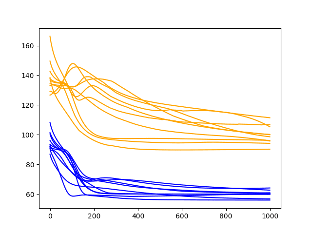
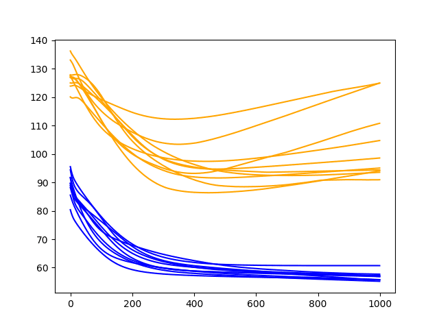
A line plot of the test and train RMSE scores each epoch is also created.
This is more telling. It shows a rapid decrease in test RMSE to about epoch 500-750 where an inflection point shows a rise in test RMSE almost across the board on all runs. Meanwhile, the training dataset shows a continued decrease to the final epoch.
These are good signs of overfitting of the training dataset.
Diagnostic Results with 1000 Epochs and 2 Neurons
Let’s see if this trend continues with even more neurons.
Diagnostic of 1000 Epochs and 3 Neurons
This section looks at the same configuration with the number of neurons increased to 3.
We can do this by setting the n_neurons variable in the run() function.
1
n_neurons=3
Running this configuration prints the RMSE scores from the final epoch of each run.
Note: Your results may vary given the stochastic nature of the algorithm or evaluation procedure, or differences in numerical precision. Consider running the example a few times and compare the average outcome.
The results are similar to the previous section; we do not see much general difference between the final epoch test scores for 2 or 3 neurons. The final train scores do appear to be lower with 3 neurons, perhaps showing an acceleration of overfitting.
The inflection point in the training dataset seems to be happening sooner than the 2 neurons experiment, perhaps at epoch 300-400.
These increases in the number of neurons may benefit from additional changes to slowing down the rate of learning. Such as the use of regularization methods like dropout, decrease to the batch size, and decrease to the number of training epochs.
1
2
3
4
5
6
7
8
9
10
0) TrainRMSE=55.686242, TestRMSE=90.955555
1) TrainRMSE=55.198617, TestRMSE=124.989622
2) TrainRMSE=55.767668, TestRMSE=104.751183
3) TrainRMSE=60.716046, TestRMSE=93.566307
4) TrainRMSE=57.703663, TestRMSE=110.813226
5) TrainRMSE=56.874231, TestRMSE=98.588524
6) TrainRMSE=57.206756, TestRMSE=94.386134
7) TrainRMSE=55.770377, TestRMSE=124.949862
8) TrainRMSE=56.876467, TestRMSE=95.059656
9) TrainRMSE=57.067810, TestRMSE=94.123620
A line plot of the test and train RMSE scores each epoch is also created.
Diagnostic Results with 1000 Epochs and 3 Neurons
Summary of Results
Again, we can objectively compare the impact of increasing the number of neurons while keeping all other network configurations fixed.
In this section, we repeat each experiment 30 times and compare the average test RMSE performance with the number of neurons ranging from 1 to 5.
Running the experiment prints the summary statistics for each configuration.
Note: Your results may vary given the stochastic nature of the algorithm or evaluation procedure, or differences in numerical precision. Consider running the example a few times and compare the average outcome.
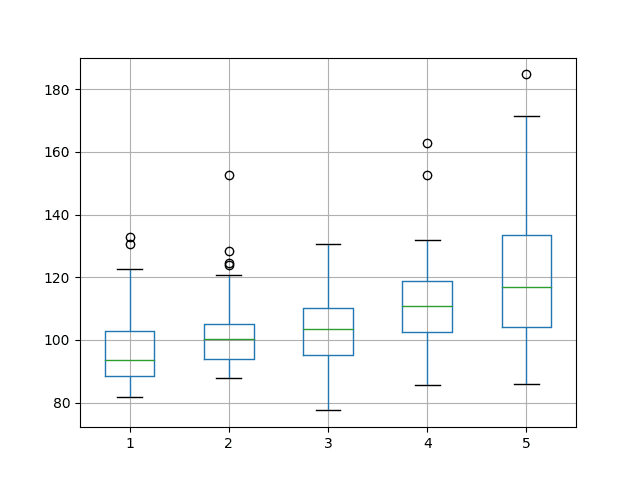
From the mean performance alone, the results suggest a network configuration with 1 neuron as having the best performance over 1000 epochs with a batch size of 4. This configuration also shows the tightest variance.
max 132.934054 152.588092 130.551521 162.889845 184.678185
The box and whisker plot shows a clear trend in the median test set performance where the increase in neurons results in a corresponding increase in the test RMSE.
Box and Whisker Plot Summarizing Neuron Results
Summary of All Results
We completed quite a few LSTM experiments on the Shampoo Sales dataset in this tutorial.
Generally, it seems that a stateful LSTM configured with 1 neuron, a batch size of 4, and trained for 1000 epochs might be a good configuration.
The results also suggest that perhaps this configuration with a batch size of 1 and fit for more epochs may be worthy of further exploration.
Tuning neural networks is difficult empirical work, and LSTMs are proving to be no exception.
This tutorial demonstrated the benefit of both diagnostic studies of configuration behavior over time, as well as objective studies of test RMSE.
Nevertheless, there are always more studies that could be performed. Some ideas are listed in the next section.
Extensions
This section lists some ideas for extensions to the experiments performed in this tutorial.
If you explore any of these, report your results in the comments; I’d love to see what you come up with.
Dropout. Slow down learning with regularization methods like dropout on the recurrent LSTM connections.
Layers. Explore additional hierarchical learning capacity by adding more layers and varied numbers of neurons in each layer.
Regularization. Explore how weight regularization, such as L1 and L2, can be used to slow down learning and overfitting of the network on some configurations.
Optimization Algorithm. Explore the use of alternate optimization algorithms, such as classical gradient descent, to see if specific configurations to speed up or slow down learning can lead to benefits.
Loss Function. Explore the use of alternative loss functions to see if these can be used to lift performance.
Features and Timesteps. Explore the use of lag observations as input features and input time steps of the feature to see if their presence as input can improve learning and/or predictive capability of the model.
Larger Batch Size. Explore larger batch sizes than 4, perhaps requiring further manipulation of the size of the training and test datasets.
Summary
In this tutorial, you discovered how you can systematically investigate the configuration for an LSTM network for time series forecasting.
Specifically, you learned:
How to design a systematic test harness for evaluating model configurations.
How to use model diagnostics over time, as well as objective prediction error to interpret model behavior.
How to explore and interpret the effects of the number of training epochs, batch size, and number of neurons.
Do you have any questions about tuning LSTMs, or about this tutorial?
Ask your questions in the comments below and I will do my best to answer.
Develop Deep Learning models for Time Series Today!
Thanks for such a detailed and helpful tutorial. I would like ask: when tune hyperparamters, why in the order of epoch number, batch size, then Number of neurons? Is there anything special about this order? Thanks a lot!
I am doing electrical load forecasting for my company which has a larger agriculture area and load in agriculture is majorly depends on rainfall.We are taking rainfall as one of the input parameters.
The model is working fine(showing 4-6% variation from actual) when there is slight change in rainfall but giving approx 16-20% variation when there is a sudden change in rainfall. Please guide me for the same.(I am taking approx 2.5 year data for training and testing).
CAPACITY AND TRAINABILITY IN RECURRENT NEURAL NETWORKS
section:2.1.1
we draw datasets of binary inputs X and target binary labels Y at uniform from the
set of all binary datasets.Number of samples, b, is treated as a HP and
in practice the optimal dataset size is very close to the bits of mutual information between true and predicted labels. For each value of b
the RNN is trained to minimize the cross entropy of the network output with the true labels. We write the output of the RNN for all inputs as ^Y = f (X), with corresponding random variable ^ Y. We are interested in the mutual information I between the true class labels and the class labels predicted by the RNN.
line 137, in
results[str(e)] = experiment(repeats, series, e)
line 104, in experiment
lstm_model = fit_lstm(train_trimmed, batch_size, epochs, 1)
line 81, in fit_lstm
model.fit(X, y, epochs=1, batch_size=batch_size, verbose=0, shuffle=False)
File “C:\Anaconda3\lib\site-packages\keras\models.py”, line 654, in fit
str(kwargs))
TypeError: Received unknown keyword arguments: {‘epochs’: 1}
Is there something wrong?
Nice blog post once again. What is the size of the data set that you are using? What is the maximum data size that one can use with your example if I have a system with 8GB RAM?
Great work! I have a question regarding batch_size. I think that only one batch_size is reasonable for this case because stateful is true. If batch_size is 4, there are 4 states separately. That means 4 states don’t share each other. Although every sample has connection with the next sample sequently, every sample is connected the quaternary next sample.
I think that the batch_size depends on not user tuning parameter but dataset design relative to the number of sequence set.
When batch_size is 4 and stateful is true, output of LSTM is weight_count * batch_size. This means that there are 4 different and independent states. It seems good for the following dataset :
A1-B1-C1-D1-A2-B2-C2-D2-A3-B3-C3-D3
– sample is 12
– batch_size is 4
– sequence set is 4
Because A isn’t relative to others in sequence, the next of A1 should be not B1 but A2. For this we have to choose batch_size as 4.
For each epoch,
A1-A2-A3 and reset
B1-B2-B3 and reset
C1-C2-C3 and reset
D1-D2-D3 and reset
Your example is one sequence set like:
A1-A2-A3-A4-A5-A6-A7-A8-A9-A10-A11-A12
If we set batch_size as 4, state is transferred as the following:
A1-A5-A9 and reset
A2-A6-A10 and reset
A3-A7-A11 and reset
A4-A8-A12 and reset
So, I think that batch_size should be 1 in your dataset. Other batch_size values are invalid.
I agree with the first part, it makes sense to reset state at the natural end of a sequence.
I also agree that with the dataset used that there is no natural end to the sequence other than the end of the data, so no state resets are needed.
I disagree that you “have to have” a batch size of 1. We can have a batch size of 1. We can also have a batch size equal to the sequence length.
My previous point is that batch size does not matter when stateful=True because we manage exactly when the state is reset. It does not matter what batch size is used, as long as the state is reset at the natural end of the sequence.
Yes, you are right, there is a bug. The regime of resetting state after each batch of 4 input patterns does not make sense. I’ll schedule time to fix the examples and re-run the experiments.
Thanks for pointing this out and thanks for having the patients to help me see what you saw.
UPDATE: There is no fault, all weight updates are occurring within one epoch regardless of batch size.
Cool post! I already learnt a lot from your blogs.
I have 2 questions regarding this post, I hope you can help me:
1. Why aren’t you specifying activation functions in your model layers (for the LSTM layer for example?) I read on the keras docs that no activation function is used if you don’t pass one. It seems to me that a tanh activation would fit the [-1,1] scaling?
2. Do you always remove the increasing trend from the data?
When reversing difference for predicitions, isn’t it wrong to reverse it using the raw values? Instead, shouldn’t you use the last prediction to reverse the difference?
Like, instead of yhat = yhat + history[-interval] it is yhat = yhat + predictions[-interval]?
Thank you Dr. Jason for the great blog. Is it possible to use GPU for this example? If so, how can I apply it! I appreciate your help. The reason I want to use GPU is that I need to get results faster. I am using google compute engine with 6vCPUs and 39 GB memory.
Many thanks for your great tutorial.
I have a question regarding updating the model after making a prediction on each timestep of the test dataset. Could you please explain which line of the code is responsible for doing this; I mean the line that implements this statement: “… then the actual expected value from the test set will be taken and made available to the model for the forecast on the next time step.”
I want to implement proper hyper parameter tuning mechanism for LSTM time series forecasting.
But I am facing difficulties using grid search for time series model.
Also I dont find proper guidelines for using Bayesian optimization in LSTM time series forecasting.
Thank you in advance
Hi Jason!
Can we use GridSearchCV to tune LSTM Hyperparameters with Keras for Time Series Forecasting?
or we can not do this because for GridSearchCV we need cross validation but in this case we can not use cross validation (time seies)
~/anaconda3/lib/python3.6/site-packages/sklearn/model_selection/_search.py in fit(self, X, y, groups, **fit_params)
638 error_score=self.error_score)
639 for parameters, (train, test) in product(candidate_params,
–> 640 cv.split(X, y, groups)))
641
642 # if one choose to see train score, “out” will contain train score info
~/anaconda3/lib/python3.6/site-packages/sklearn/externals/joblib/parallel.py in __call__(self, iterable)
787 # consumption.
788 self._iterating = False
–> 789 self.retrieve()
790 # Make sure that we get a last message telling us we are done
791 elapsed_time = time.time() – self._start_time
~/anaconda3/lib/python3.6/site-packages/sklearn/externals/joblib/parallel.py in retrieve(self)
697 try:
698 if getattr(self._backend, ‘supports_timeout’, False):
–> 699 self._output.extend(job.get(timeout=self.timeout))
700 else:
701 self._output.extend(job.get())
~/anaconda3/lib/python3.6/multiprocessing/pool.py in get(self, timeout)
642 return self._value
643 else:
–> 644 raise self._value
645
646 def _set(self, i, obj):
~/anaconda3/lib/python3.6/multiprocessing/pool.py in _handle_tasks(taskqueue, put, outqueue, pool, cache)
422 break
423 try:
–> 424 put(task)
425 except Exception as e:
426 job, idx = task[:2]
Dear Jason,
To make sure I am interpreting things as I should , what is th difference between neurons , layers and hidden states?
I am asking because the inner structure of an LSTM is completely different from any other NN and is composed of mulptiple gates rather than “neurons”.
Am I missing Something here?
ok thank you Jason. I understand then that a neuron in LSTM does exactly the same thing as in feedforward NN, that is: computing the activation function. The difference is that in LSTM, the neuron is far more complex and is composed of 4 gates and processes a hidden vector that is recursively fed to the neuron itself.
Dear all ,
How should I reshape my dataset if the objective is to use the last M points to predict the next N points for multiple time series at once. In my project, I am dealing with 20 time series at the same time.
Thank you very much for you help!!
May i know why do we need to reset the model after evaluating?i know that we need to reset when performing model.fit , but why do so on evaluating as well? thank you
It looks like there is no one optimal combination of Epochs, Batch Size and Neurons. Is this a correct observation?
Also, does tuning so much on the given training and testing set lead to overfitting to these sets? Should there be training-validation-test combination where you would check findings with the test set in the end?
Hello Jason, thank you for your dedication I have learned a lot from you.
Currently I’m trying to predict the energy output of wind turbines for an interval of every 15 minutes using LSTM. Are there any optimization methods, loss functions among other parameters you would particularly suggest for such a case study? my data set is a data set of dimensions (57000, 17). thank you
Hi Sir, thank you very much for all your content. This is my first time learning machine learning specifically LSTM.
Is it possible to tune these hyperparameters simultaneously?
ei. for each epoch (say 500, 1000, 3000) try batch sizes of 1,2,3 and for each batch size set neurons to 1,2,3,4
With this method, can we assess which of the following combinations yield better result? I am aware that this is would take a lot of time to do but I am curious if this is plausible and sensible to perform.
I have not difference the series because there is no trend in this series. I calculated statistics of partitioned time series data and used ADF test, the result is as follows, so I think it a stationary series.
Thanks for your sharing. I tried your codes on my jupyter notebook. Tuning epochs worked properly.
However, fit_lstm fn in tuning epochs gives a dataframe as an output.
So it is not the same fit_lstm fn in tuning batch_size. Which should have a model to predict as an output.
In my notebook it gives such an error:
‘AttributeError: ‘DataFrame’ object has no attribute ‘predict’
Am I missing something or is it because of my Keras version?
I would like to know how I can save a model and use it to forecast.
In your “Summary of Results” of the last section (the codes above “Summary of All Results”),
line 21: I want to save the last model which function “fit_lstm” output.
I modified your code to achieve this but give me error “AttributeError: ‘Series’ object has no attribute ‘predict'”, I figured out that the error was due to the model I saved was not a correct one to use, though I checked the model’s value was “<keras.models.Sequential object at 0x0000026EC…" which looks right.
Below is what I did:
# fit an LSTM network to training data
def fit_lstm(train, test, raw, scaler, batch_size, nb_epoch, neurons):
#### omitted copy of your codes here#####
# fit model
train_rmse, test_rmse = list(), list()
for i in range(nb_epoch):
model.fit(X, y, epochs=1, batch_size=batch_size, verbose=0, shuffle=False)
model.reset_states()
#### omitted copy of your codes here#####
history = DataFrame()
history['train'], history['test'] , history['model']= train_rmse, test_rmse, model
return history
### save last model to dataframe "history"
# run diagnostic experiments
def run(repeats, n_epochs, n_batch, n_neurons):
# fit and evaluate model
train_trimmed = train_scaled[2:, :]
results_run = DataFrame()
error_scores = list()
# run diagnostic tests
for i in range(repeats):
history = fit_lstm(train_trimmed, test_scaled, raw_values, scaler, n_batch, n_epochs, n_neurons)
#### omitted copy of your codes here#####
if i==0:
model_tune = history['model']
results_run['error_scores'], results_run['model_tune'] = error_scores, model_tune
return results_run
### Below out of function and loops ####
results_temp = run(repeats, n_epochs, n_batch, n_neurons)
model_tune_all = results_temp['model_tune']
model_tune = model_tune_all[-1:]
### get model_tune is <keras.models.Sequential object at 0x0000026EC… ####
forecasts = make_predictions(model_tune, n_batch, test_scaled, n_lag)
### AttributeError: 'Series' object has no attribute 'predict' ####
If I use the sequence length 3. x1,x2,x3 -> x4 = y1. Should I set batch size 3 for the fitting? I am not using stateful. The sequences are not dependent on each other so I cant have the LSTM take information from another sequence.
Your posts have helped me a lot so I want to say thank you! However I have two questions. I am training my LSTM on the sequence x0, x1, x2 -> y0 = x3 and I am using stateless. The reason I use statess is because I want to reset the state after a sequence beacause the sequences are not dependant on each other. My first question is if I am thinking correctly about stateless?
Second question, the training batch size you define when building the LSTM, is that the batch size which the states reset? Or is it resetted after each sequence?
With other words, should I train with in my case batch size 3 or can I use any batch size?
Thank you very much for your efforts
How to set the volume batch_size with this model
The number of rows in a dataset of 10000 data
Number and features 12
11 input
1 output
net = tflearn.input_data([None, 11])
net = tflearn.embedding(net, input_dim=10000, output_dim=128)
net = tflearn.lstm(net, 128, dropout=0.8)
net = tflearn.fully_connected(net, 1, activation=’sigmoid’)
net = tflearn.regression(net, optimizer=’adam’, learning_rate=0.001,
loss=’binary_crossentropy’)
Hi, i am currently building a model for time series forecastings using LSTM , is there a way to perform dynamic searches for best parameters, like gridsearch etc, we cant use grid search and etc, becaue the sequence is of importance. I would highly appreciate it if you could guide me towards the dynamic parameter tuning for LSTM time series model in python.
“For univariate forecasting problems, all deep learning methods are out-performed by classical methods like SARIMA and ETS. Even naive methods.” — But how about multivariate forecasting problems? I mean, if I have several features (lag1 of multivariate time series), and I want to use them to predict one feature (a time series) among the features, is deep learning methods still not better than the SARIMA?
Actually, I’m a guy who studied ARIMA, VAR, ETS first, then came to deep learning. At the beginning of my deep learning study, I thought I found a new continent, but now I’m feeling sad.
Appreciate your answer — “I have found CNNs, CNN-LSTMs and ConvLSTMs can perform well for multivariate data.”
Moreover, could I ask, how are they performed for multivariate data compare to VAR(vector autoregression)? Thank you.
By the way, when you replied Patrão — “I have book in the works to really make this concrete.”, which book are you referring? I already bought your 12 books yesterday, so I can found CNN-LSTMs in book “long_short_term_memory_networks_with_python”, but I can’t find ConvLSTMs and the applications on multivariate time series data by using CNNs, CNN-LSTMs, and ConvLSTMs in this book. Also, when I take a quick review of the book “time_series_forecasting_with_python”, I can’t find any deep learning methods on multivariate time series because this book is all about classical time series methods. I’m not making a complaint here, but I really need someone to guide me to make my hands dirty onmultivariate time series data by leveraging CNNs, CNN-LSTMs, and ConvLSTMs methods. Thank you!
Hi, Jason. Do you have some examples of using a CNN, CNN-LSTM or ConvLSTM on time series forecasting for univariate forecasting problems? Thank you so much!
Hi Jason.
Many thanks for your great tutorials.
Could you please let me know if you have an example using Scikit-Optimize (skopt) to tune the hyper-parameters with the dataset?
I have a question about the correct time to scale data. In your LSTM book, you state “It would not be appropriate to scale the series after it has been transformed into a supervised learning problem as each series would be handled differently, which would be incorrect.” However, I see in this example, that the scaling occurs after the data has been transformed to a supervised learning problem. In this case, does the timing not matter? If so, would you please explain why?
In my use case of LSTM, I am observing something unusual. It intuitively makes sense to have the train RMSE to be less than the test RMSE. But in my case, I have the train RMSE to be greater than the test RMSE.
For instance,
After running for 4 epochs
Train RMSE: 0.097 Test RMSE: 0.046
The split of my training and testing data is 2/3 and 1/3.
I can think of the following cases why this is happening
a) The test cases are very similar to the train cases, therefore the prediction accuracy is high
b) The number of test cases are not enough.
What are your thoughts on this? Do you think it is a problem?
Hi Jason,
Thank you very much for this tutorial. I have one question and that is how we can evaluate the model performance since we can’t do a k-fold cross validation.Is it OK just testing it on the test dataset?
This post has been very helpful! I do have a question. I am attempting to adapt what you have here to a different dataset, one that does not have much of a discernible trend. I have that, in other algorithms with my dataset, that taking the log10 is the only transformation i need to apply to get good output. I am wondering how i might configure the
1
2
3
4
5
6
7
8
9
foriinrange(len(output)):
yhat=output[i,0]
# invert scaling
yhat=invert_scale(scaler,X[i],yhat)
#invert differencing
yhat=yhat+raw_data[i]
# store forecast
predictions.append(yhat)
in the evaluate formula to work for inverting the log10, rather than the difference of yhat and raw_data[i]? Or is taking the log unnecessary for this type of model?
Which one is the part in which we are fitting the model? Is it:
1)LSTM(neurons, batch_input_shape=(batch_size, X.shape[1], X.shape[2]), stateful=True)
or 2) model.fit(X, y, epochs=1, batch_size=batch_size, verbose=0, shuffle=False)?
I’m confused because in the second part is looks like we are setting the epochs to 1. Can you explain what we are doing there?
I’m having some trouble understanding the code in this bit of the script. I’m trying to understand each part of your entire code very carefully, but for some reason, I have a hard time visualizing this part. I apologize if this is a trivial question:
a) What exactly is train_scaled[2:, :]?
b) at the end of the lst.fit part why do we specify the number 1? what does that refer to?
code:
for r in range(repeats):
# fit the model
train_trimmed = train_scaled[2:, :]
lstm_model = fit_lstm(train_trimmed, batch_size, epochs, 1)
I am new to RNN and LSTM. I am solving a problem (supervised regression), which predicts a parameter using 23 features. Please suggest a starter numbers for input/output neurons, layers, activation fn, loss, optimizer, epochs.
Dear Jason,
I figured out my other questions, but found another one:
What does this do?
# forecast the entire training dataset to build up state for forecasting
…
lstm_model.predict(train_reshaped, batch_size=batch_size)
I’m not quite sure why you would be forecasting training data (since you’re using it to train your model) – why not just forecast the test data directly? What is the thought process behind this?
Thank you Jason :). I assumed it wasn’t required, but needed to maker sure.
With your tutorials I’ve managed to build a number of lstm’s with multiple input, multiple output, multiple lag timesteps, and multiple predictions into the future. All differenced, hot-encoded when needed, and scaled. I’m now just working on creating a harness that can systemically search out different parameter and hyperparameter configurations. I’ve decided to buy one of your books to show my appreciation. Any suggestions as to a book with lots of project examples (especially similar to problems found in meteorological study)?
Hello Jason,
done! Looks like a great book. I’m going to go through it linearly like you suggest in your preface. You mention that it might be ok to shoot you an email regarding some specific questions (if they’re not answered by checking them out in the materials mentioned in the further reading sections) – I wouldn’t want to bother you too much, however. Is there perhaps an online message board associated with each book?
Right now I am trying to implement the LSTM algorithm to a different time-series data. I have tried to build the model using R instead of python. Although, I came across to a tutorial (https://www.r-bloggers.com/time-series-deep-learning-forecasting-sunspots-with-keras-stateful-lstm-in-r/) where it suggested numbers of data exploration, one of it is ACF and PACF review.
It does not seem you have done the same ACF and PACF analysis prior to constructing the model. Have you confirmed it in advance that the data is suitable for LSTM model? Or is there another way to construct the model even though the data does not in fulfill the ACF criteria?
I’m a little confused. In the Summary of Results section, I know that this code is not required. But I wonder how important is the state of the network to the later prediction?
In keras, LSTM is trained with a certain batch_size, so I have to input batch_size in the end when I predict? For example, if the state stored by the network is batch_size, what will happen if the data I input is not that size?
Got a few questions about your choice of data preparation methodology –
1- What is the purpose of the lag? Also, why did you choose differencing to remove the trend? Ultimately, are you trying to find the difference between two days? How would you convert the difference back into un-differenced values?
2- The supervised learning aspect, gives you 2 columns of data where the value in the first column is supposed to be the observation from the previous time step to be used as input to find the value in the second column?
Read those articles, and definitely making a clearer picture of how my LSTM will be setup.
A quick follow up on the difference transformations – using t-1 -> t-48 to predict t -> t+12 I feel that for my data certain trends and time of year are important to the output, and so will have day of the year, and day of the week as part of my feature set. Since this is a univariate prediction problem I only need to predict the value, but utilizing multiple features at every one of the previous timesteps. The data is non-linear and generally increasing over time, but not always.
Every feature needs to be normalized according to that specific feature, correct? (Getting somewhat side-tracked here but…) For day of the year, I would use min-max scaler for between -1 and 1 does that make any sense to do?
Ok sorry, back to my original thought, if I am predicting a sequence, how would the inverse difference work if the previous timestep value would be that of a predicted value? My thinking was to just do min-max scaler for each sample set, or is that overkill?
Ahh – ok, so using the predicted values to calculate the difference going forward. Next I have to figure out whether or not I am actually going to use an encoder/decoder model and which loss functions and optimizers to use
Oh sorry – one more question on the difference transformation – the network is trained on the inverse difference values correct?
So –
– Difference input data
– Scale input data
– Make prediction
– Unscale output data
– Inverse difference of unscaled output data
– use RMSE to determine the error
– Train network based on error
Or is the Keras LSTM handling the optimization and we are simply unscaling and running the inverse difference to get the output, then using RMSE to determine how accurate the network is?
For Shampoo sales, you have only one sample. I remember you said that ” if there is one sample and the batch size is > 1, The batch size will be 1″.
Why the batch size is 2, 4 here when only one sample (24 observations) is available.
When batch_size is four, does it mean that four same samples (training examples)will be propagated into the network ? Since one epoch = one forward pass and one backward pass of all the training examples. Weights parameters will be updated four times in one batch ???
I have enjoyed your blog posts, thank you for all the hard work. As my program is building it occurred to me that we are isolating each tuning variable and then assessing the performance based on static values for the other values.
So my questions are:
1) Is there an order which in tuning these isolated variables? Such as, tune batch size first since it is dependent on being a divisor of test/train data. Then train the number of epochs (for whichever reason), then train the number of neurons? This is the intuitive/manual approach without destroying my computational time.
2) I want to eventually create an automated script to optimize the tuning parameters for me, but I want to figure out a way that doesn’t take days to run due to computational limitations. (I’m trying to avoid Grid searching: analyze all possibilities of X, given possibilities Y/Z; then analyze all possibilities of Y, given possibilities of X/Z; then analyze all possibilities of Z, given variables of Y/X). My first thought is to try random starting values and then apply Newton’s Min/Max finding? Any method that has worked well for you to date?
Either way, I will continue to test the suggested tuning changes and start working on the tuning automation. I’ll let you know of my results once I get them.
I wounder if I could apply the concept of LSTM between the output layer units. To explain more, I am predicting the time series based on properties of the system.
Do you believe that assume that you have the best features to train your model (time-series). Is it good approach build a model that stop only when all instances reach a max error?
Is there any technical reason to refer to the first input of the LSTM layer as “neurons” instead of “units”? Per the Keras documentation: units: Positive integer, dimensionality of the output space. Is it just a matter of taste?
I have a out of context question. Is data extraction from scratch a job for data analysts or is it done by us developers itself? Preprocessing is not a big issue but formation of data seems like a tedious task.
how to make multivariate time series data stationary?only need to make outputs stationary or whole dataset should be stationary ?need some tutorial for this.
Hi, Jason! I have a question regarding the method you use: what is the justification behind using just one neuron when tuning the number of epochs and batch size? Couldn’t we have started with a higher number?
Thank you in advance, and congrats for this great blog.
Hello Jason, I had a question about what LSTM neurons learn in each layer. How can you know what they learn in the first layer or in the hidden layers?
In here, you tuned number of epochs first, and then batch size and number of nodes.
How did you decided the order of tuning?
In my experience, optimized value for the epochs varied due to the batch size and number of nodes.
Nice post!
A question: How do I deal with all the NaN values that are naturally created because of the shifting? Keras does not like NaN values.
I used lag=30. I would change the code so that lag(=1) won’t be hardcoded. There are couple of places where the code needs to be changed if you use lag different than 1.
Dear Jason,
Thank you for sharing your amazing tutorials and lessons. I really appreciate it as I am digging more and more into the neural network world!
I am working on a large time-series dataset, for which I am trying to understand the possibility of LSTM predictions. I created a Train and Test set with an 80/20 rule. However, the parameter tuning is slowed down by the training’s size (more than 100k elements).
Would it be an acceptable – and generalizable – solution to tune the LSTM on a subset of this dataset and then apply it to the larger collection?
Thank you very much in advance 🙂
Thank you for this informative article!!!
I have a doubt regarding scaling preprocessing step. In this problem, there is only 1 feature and input, output are of same range.
Does scaling really helps in such scenarios?
Dear Jason, wonderful tutorial, thank you very much! Would you be so kind and be the first in the literature to adapt the tutorial from a univariate data set to a multivariate data set?
Really great work Jason. I think the most important thing you have done here is taught people to use a framework for testing many combinations of parameters. It’s not like using a diving rod, the computer can crunch the numbers (and without you sitting and watching models train) as long as you do the work upfront to set up a good testing structure.
Hey Jason. I’m a computer science student from Colombia and I just wanted to thank you for the effort you put into this. Your blogs have saved me many times and have made my understanding and love for ML grow exponentially.
Dear Dr.Jason,
I have encountered a few problems and wish if you could help me out. it might be a little out of scope for this discussion.This is the model architecture I am working with but I want it in a function so that I can later use it after performing bayesian optimization but I always get history not defined for this function.
That’s weird. I can’t see what’s wrong. Your model.fit() should return a history object (you can try “print(type(history))” after fit to confirm) and therefore “history.history” should give you the data you want.
I tried this for a different dataset. It worked perfectly fine for LSTM but then I tried it using GRU instead of LSTM. My question is about the GRU model.
Everything went OK for a batch size of 12 (factor of the sizes of the training and test dataset) but the performance for a batch size of 6 was better, I mean, smaller mean, median and minimum RMSE for the test set. However, for the latter batch size the RMSE vs. epochs plot did not look that good, since some of the training curves overcame the test curves up to 200 epochs, and they even showed an increasing trend. I found this odd because 200 is precisely the optimal number of epochs that I got. For further iterations though, the trend in error is decreasing for the training set and increasing for the test set, showing the expected overfitting.
Is this behaviour normal somehow or this shouldn’t be happening?
I’ve enjoyed reading your tutorial and learning a lot, thank you so much! It would be nice to see if you can also share how you do the hyperparameter tuning for multivariate LSTM time series! Thanks!
I’m from Brazil, and your tutorials have been incredibly helpful to me. Currently, I’m working on an LSTM network project using two different evaluation methods: sliding window and expanding window. However, I’m facing some difficulties in tuning my network.
I have a dataset with four years of daily data, using the last year as the test set. The sliding window step is 7 days, which sets my forecast horizon to 7 days with daily frequency. To complete a full year of forecasting, it takes 53 iterations, meaning the model is retrained 53 times to cover the entire test year.
How can I visualize the diagnostic plots in this scenario? Does this mean I need to look at 53 different plots to analyze the performance of each model I test?
It’s still a bit unclear for me on how to make this work…
Hi Antoniel…Hi! It’s great to hear that my tutorials have been helpful to you, and I’m glad you’re working on such an interesting LSTM project.
Let’s break this down to simplify the challenge of visualizing the diagnostic plots for the sliding window approach.
### 1. **Understanding the Challenge**
Since your forecast horizon is 7 days and you’re retraining the model 53 times to cover the entire test year, visualizing the performance can become overwhelming if you look at each iteration separately. But instead of generating 53 individual plots, you can:
– **Aggregate performance**: Focus on summary statistics (like average RMSE, MAE, or MSE) across all 53 iterations to get an overall sense of model performance.
– **Combine predictions**: Combine the predictions from all 53 iterations into a single plot for visual comparison against the actual values for the full year.
### 2. **How to Visualize Diagnostics**
Here’s how you can approach visualization efficiently:
#### A. **Overall Performance Plot**
You can aggregate the predicted vs. actual values for all 53 windows and plot them together. This will give you a comprehensive view of the entire year’s predictions, without having to generate 53 separate plots.
python

import matplotlib.pyplot as plt
# Assuming y_true and y_pred are your actual and predicted values across all windows
plt.plot(y_true, label='Actual')
plt.plot(y_pred, label='Predicted')
plt.legend()
plt.title('Predicted vs Actual Values for Full Year')
plt.show()
#### B. **Error Metrics Over Time**
You can also plot error metrics like RMSE or MAE across the 53 iterations to see how your model’s performance changes over time. This helps in identifying patterns or trends in model accuracy.
python

import numpy as np
# Assuming rmse_list contains RMSE values for each window
plt.plot(np.arange(len(rmse_list)), rmse_list, label='RMSE')
plt.title('RMSE over Time (Sliding Window)')
plt.xlabel('Window Iteration')
plt.ylabel('RMSE')
plt.show()
#### C. **Boxplot of Errors**
A boxplot can summarize the distribution of errors (residuals) across the windows in a single visualization.
python

import seaborn as sns
# Assuming errors is a list of residuals from each window
sns.boxplot(data=errors)
plt.title('Residuals Across Sliding Windows')
plt.show()
### 3. **Expanding Window Strategy**
If you’re using the expanding window evaluation method, the process is similar but the model is trained on progressively more data over time. You can use the same plotting strategies as above but may want to compare the sliding window and expanding window methods side-by-side to determine which gives better results.
### 4. **Conclusion**
Rather than creating 53 separate plots, aim to summarize and aggregate the results so you can visualize trends and overall performance more clearly. Focus on a combination of actual vs. predicted plots, error metrics over time, and statistical summaries like boxplots.


Awesome Work!
Thanks John!
Thanks for such a detailed and helpful tutorial. I would like ask: when tune hyperparamters, why in the order of epoch number, batch size, then Number of neurons? Is there anything special about this order? Thanks a lot!
Probably start with the setting a large capacity for the model then tune the learning rate:
https://machinelearningmastery.com/framework-for-better-deep-learning/
Hi Json,
Can we intentionally emphasize on one perticular inpur parameter for forecasting???
Typically no. Why?
Hi Jason,
I am doing electrical load forecasting for my company which has a larger agriculture area and load in agriculture is majorly depends on rainfall.We are taking rainfall as one of the input parameters.
The model is working fine(showing 4-6% variation from actual) when there is slight change in rainfall but giving approx 16-20% variation when there is a sudden change in rainfall. Please guide me for the same.(I am taking approx 2.5 year data for training and testing).
Thanks in advance.
Perhaps try some of the suggestions here:
https://machinelearningmastery.com/start-here/#better
CAPACITY AND TRAINABILITY IN RECURRENT NEURAL NETWORKS
section:2.1.1
we draw datasets of binary inputs X and target binary labels Y at uniform from the
set of all binary datasets.Number of samples, b, is treated as a HP and
in practice the optimal dataset size is very close to the bits of mutual information between true and predicted labels. For each value of b
the RNN is trained to minimize the cross entropy of the network output with the true labels. We write the output of the RNN for all inputs as ^Y = f (X), with corresponding random variable ^ Y. We are interested in the mutual information I between the true class labels and the class labels predicted by the RNN.
can any one help me in solving this ???
See this:
https://machinelearningmastery.com/information-gain-and-mutual-information/
trully very nice toturial.
also, you can find my “time series prediction with hyperparameter tuning by Bayesian optimization in MATLAB” Here:
https://www.mathworks.com/matlabcentral/fileexchange/87137-lstm-time-series-prediction-with-bayesian-optimization
Thanks for sharing.
line 137, in
results[str(e)] = experiment(repeats, series, e)
line 104, in experiment
lstm_model = fit_lstm(train_trimmed, batch_size, epochs, 1)
line 81, in fit_lstm
model.fit(X, y, epochs=1, batch_size=batch_size, verbose=0, shuffle=False)
File “C:\Anaconda3\lib\site-packages\keras\models.py”, line 654, in fit
str(kwargs))
TypeError: Received unknown keyword arguments: {‘epochs’: 1}
Is there something wrong?
You need to upgrade to Keras v2.0 or higher.
You should replace model.fit(X, y, epochs=1, …) for model.fit(X, y, nb_epoch=1…) It worked perfectly for me.
The example was updated to use Keras v2.0 which changed the “nb_epochs” argument to now be “epochs”.
Hi Jason, another great material. Thanks for that!
Just a doubt… instead of model.fit(X, y, epochs=1, …), should it be model.fit(X, y, epochs=i, …)?
Best regards
No, as we are enumerating the number of epochs manually.
Nice blog post once again. What is the size of the data set that you are using? What is the maximum data size that one can use with your example if I have a system with 8GB RAM?
The examples use small <1 MB datasets.
The size of supported datasets depends on data types, number of rows and number of columns.
Consider doing some experiments with synthetic data to find the limits of your system.
Amazing tutorial as always. Would you have an example of running the LSTM on a multivariate regression problem like the Walmart’s on Kaggle (https://www.kaggle.com/c/walmart-recruiting-store-sales-forecasting) ?
There should be some examples on the blog soon.
Great work! I have a question regarding batch_size. I think that only one batch_size is reasonable for this case because stateful is true. If batch_size is 4, there are 4 states separately. That means 4 states don’t share each other. Although every sample has connection with the next sample sequently, every sample is connected the quaternary next sample.
For example,
1 > 5 > 9
2 > 6 > 10
3 > 7 > 11
4 > 8 > 12
Sorry, I’m not sure I understand your question, perhaps you can restate it.
We are using stateful LSTMs and regardless of the batch size, state is only reset when we reset it explicitly with a call to model.reset_states()
I think that the batch_size depends on not user tuning parameter but dataset design relative to the number of sequence set.
When batch_size is 4 and stateful is true, output of LSTM is weight_count * batch_size. This means that there are 4 different and independent states. It seems good for the following dataset :
A1-B1-C1-D1-A2-B2-C2-D2-A3-B3-C3-D3
– sample is 12
– batch_size is 4
– sequence set is 4
Because A isn’t relative to others in sequence, the next of A1 should be not B1 but A2. For this we have to choose batch_size as 4.
For each epoch,
A1-A2-A3 and reset
B1-B2-B3 and reset
C1-C2-C3 and reset
D1-D2-D3 and reset
Your example is one sequence set like:
A1-A2-A3-A4-A5-A6-A7-A8-A9-A10-A11-A12
If we set batch_size as 4, state is transferred as the following:
A1-A5-A9 and reset
A2-A6-A10 and reset
A3-A7-A11 and reset
A4-A8-A12 and reset
So, I think that batch_size should be 1 in your dataset. Other batch_size values are invalid.
I agree with the first part, it makes sense to reset state at the natural end of a sequence.
I also agree that with the dataset used that there is no natural end to the sequence other than the end of the data, so no state resets are needed.
I disagree that you “have to have” a batch size of 1. We can have a batch size of 1. We can also have a batch size equal to the sequence length.
My previous point is that batch size does not matter when stateful=True because we manage exactly when the state is reset. It does not matter what batch size is used, as long as the state is reset at the natural end of the sequence.
Yes, you are right, there is a bug. The regime of resetting state after each batch of 4 input patterns does not make sense. I’ll schedule time to fix the examples and re-run the experiments.
Thanks for pointing this out and thanks for having the patients to help me see what you saw.
UPDATE: There is no fault, all weight updates are occurring within one epoch regardless of batch size.
Update I have taken a much closer look at this code (it was written months ago).
I believe there is no fault.
Take a close look at the loop for running manual epochs.
Although the batch sizes vary, we are performing one entire epoch + all weight updates before resetting state.
Great blog post!
Thanks Sebastian.
Hi Jason,
Cool post! I already learnt a lot from your blogs.
I have 2 questions regarding this post, I hope you can help me:
1. Why aren’t you specifying activation functions in your model layers (for the LSTM layer for example?) I read on the keras docs that no activation function is used if you don’t pass one. It seems to me that a tanh activation would fit the [-1,1] scaling?
2. Do you always remove the increasing trend from the data?
Thanks a lot!
I am using the default for LSTMs which are tanh and sigmoid.
Yes, making time series data stationary is a recommended in general.
Hi Jason,
very nice post, but still got a question.
When reversing difference for predicitions, isn’t it wrong to reverse it using the raw values? Instead, shouldn’t you use the last prediction to reverse the difference?
Like, instead of yhat = yhat + history[-interval] it is yhat = yhat + predictions[-interval]?
Or am I misunderstanding something?
Freetings
Yes, but if you have the real observations for a past time step, we should use them instead to better reflect the “real” level.
Does that help?
Thank you Dr. Jason for the great blog. Is it possible to use GPU for this example? If so, how can I apply it! I appreciate your help. The reason I want to use GPU is that I need to get results faster. I am using google compute engine with 6vCPUs and 39 GB memory.
Perhaps. The GPU configuration is controlled by the library used by Keras, such as TensorFlow.
I have found that it is better to run models sequentially on the GPU and instead use multiple GPUs/servers to test configurations.
Many thanks for your great tutorial.
I have a question regarding updating the model after making a prediction on each timestep of the test dataset. Could you please explain which line of the code is responsible for doing this; I mean the line that implements this statement: “… then the actual expected value from the test set will be taken and made available to the model for the forecast on the next time step.”
The model is not updated after making a prediction in this post.
This is called updating a model, see an example here:
https://machinelearningmastery.com/update-lstm-networks-training-time-series-forecasting/
By that line, I meant that we are adding observations to the history used by the model for making the next prediction.
Thank you so much for this wonderful tutorial.
Can you please help me to implement Grid search and Bayesian optimization approach for LSTM hyper parameter tuning.
Thank you in advance.
What problem are you having exactly?
I want to implement proper hyper parameter tuning mechanism for LSTM time series forecasting.
But I am facing difficulties using grid search for time series model.
Also I dont find proper guidelines for using Bayesian optimization in LSTM time series forecasting.
Thank you in advance
Sorry I don’t have an example of using Bayesian optimization for tuning LSTMs. Thanks for the suggestion.
Hi Jason!
Can we use GridSearchCV to tune LSTM Hyperparameters with Keras for Time Series Forecasting?
or we can not do this because for GridSearchCV we need cross validation but in this case we can not use cross validation (time seies)
I would recommend writing your own for-loop and using walk-forward validation to test time series forecasting models.
https://machinelearningmastery.com/backtest-machine-learning-models-time-series-forecasting/
thanks a lot Jason
hi Jason,
I think it should be possible to use gridsearchCV with LSTMs, since there is a built-in validation_split in keras.Sequential models.
gridsearchCV would be useful since it can run in parallel (also on databricks).
Do you have any simple examples of this? I get a strange error when I run grid.fit
thanks
‘model = KerasRegressor(build_fn=builder.build_LSTM_simple, verbose=verbose)
grid = GridSearchCV(estimator=model, param_grid=param_grid, n_jobs=-1)
grid_result = grid.fit(X, y)’
—————————————————————————
AttributeError Traceback (most recent call last)
in ()
—-> 1 grid_result = grid.fit(X, y)
~/anaconda3/lib/python3.6/site-packages/sklearn/model_selection/_search.py in fit(self, X, y, groups, **fit_params)
638 error_score=self.error_score)
639 for parameters, (train, test) in product(candidate_params,
–> 640 cv.split(X, y, groups)))
641
642 # if one choose to see train score, “out” will contain train score info
~/anaconda3/lib/python3.6/site-packages/sklearn/externals/joblib/parallel.py in __call__(self, iterable)
787 # consumption.
788 self._iterating = False
–> 789 self.retrieve()
790 # Make sure that we get a last message telling us we are done
791 elapsed_time = time.time() – self._start_time
~/anaconda3/lib/python3.6/site-packages/sklearn/externals/joblib/parallel.py in retrieve(self)
697 try:
698 if getattr(self._backend, ‘supports_timeout’, False):
–> 699 self._output.extend(job.get(timeout=self.timeout))
700 else:
701 self._output.extend(job.get())
~/anaconda3/lib/python3.6/multiprocessing/pool.py in get(self, timeout)
642 return self._value
643 else:
–> 644 raise self._value
645
646 def _set(self, i, obj):
~/anaconda3/lib/python3.6/multiprocessing/pool.py in _handle_tasks(taskqueue, put, outqueue, pool, cache)
422 break
423 try:
–> 424 put(task)
425 except Exception as e:
426 job, idx = task[:2]
~/anaconda3/lib/python3.6/site-packages/sklearn/externals/joblib/pool.py in send(obj)
369 def send(obj):
370 buffer = BytesIO()
–> 371 CustomizablePickler(buffer, self._reducers).dump(obj)
372 self._writer.send_bytes(buffer.getvalue())
373 self._send = send
~/anaconda3/lib/python3.6/site-packages/statsmodels/graphics/functional.py in _pickle_method(m)
AttributeError: ‘function’ object has no attribute ‘im_self’
Ok, I found that updating scikit-learn to the latest version fixed this, so I am now able to do a gridsearchCV on an LSTM.
Glad to hear it.
I show how to manually grid search LSTMs here:
https://machinelearningmastery.com/how-to-grid-search-deep-learning-models-for-time-series-forecasting/
hi jason ,
could you tell me about LSTM in which loss function ‘mean_squared_error’ is used.why it is used ..in that why cannot we measure accuracy…
This post will help clarify things for you:
https://machinelearningmastery.com/classification-versus-regression-in-machine-learning/
Dear Jason,
To make sure I am interpreting things as I should , what is th difference between neurons , layers and hidden states?
I am asking because the inner structure of an LSTM is completely different from any other NN and is composed of mulptiple gates rather than “neurons”.
Am I missing Something here?
Thank you very much
A unit is a neuron and a layer is a group of units. This is the same as an MLP.
Hidden state is a like an additional weight or local variable inside each neuron.
Does that help?
ok thank you Jason. I understand then that a neuron in LSTM does exactly the same thing as in feedforward NN, that is: computing the activation function. The difference is that in LSTM, the neuron is far more complex and is composed of 4 gates and processes a hidden vector that is recursively fed to the neuron itself.
Dear all ,
How should I reshape my dataset if the objective is to use the last M points to predict the next N points for multiple time series at once. In my project, I am dealing with 20 time series at the same time.
Thank you very much for you help!!
See this post:
https://machinelearningmastery.com/reshape-input-data-long-short-term-memory-networks-keras/
And perhaps this post:
https://machinelearningmastery.com/convert-time-series-supervised-learning-problem-python/
Hi Jason,
May i know why do we need to reset the model after evaluating?i know that we need to reset when performing model.fit , but why do so on evaluating as well? thank you
It will have state from making predictions that might not make sense for the next use of the model.
Why do you trim the data by 2 in the experiment function?
I might be removing rows with nan values given the data shift.
It looks like there is no one optimal combination of Epochs, Batch Size and Neurons. Is this a correct observation?
Also, does tuning so much on the given training and testing set lead to overfitting to these sets? Should there be training-validation-test combination where you would check findings with the test set in the end?
Yes, and results vary from problem to problem in general.
It can lead to overfitting.
Yes, this post will clarify things:
https://machinelearningmastery.com/difference-test-validation-datasets/
Hi Jason,
Great post! I’m curious as to why you scale the testing and training sets separately here, but do so as one complete data set in this post (https://machinelearningmastery.com/multivariate-time-series-forecasting-lstms-keras/).
thanks
Sometimes I do it in one step because I am focusing the tutorial on some other aspect.
Hello Jason, thank you for your dedication I have learned a lot from you.
Currently I’m trying to predict the energy output of wind turbines for an interval of every 15 minutes using LSTM. Are there any optimization methods, loss functions among other parameters you would particularly suggest for such a case study? my data set is a data set of dimensions (57000, 17). thank you
Perhaps try MAE or MSE loss functions as a start?
Hi Sir, thank you very much for all your content. This is my first time learning machine learning specifically LSTM.
Is it possible to tune these hyperparameters simultaneously?
ei. for each epoch (say 500, 1000, 3000) try batch sizes of 1,2,3 and for each batch size set neurons to 1,2,3,4
With this method, can we assess which of the following combinations yield better result? I am aware that this is would take a lot of time to do but I am curious if this is plausible and sensible to perform.
Yes, but it would require a lot of computational resources.
Hi Jason,
First, thank you for your great content. I am a beginner of the RNN, and I am a little confused with this line:
# transform train
> train = train.reshape(train.shape[0], train.shape[1])
train_scaled = scaler.transform(train)
Why do I need to reshape this, it seems the shape of it hasn’t change after the reshape.
Thank you 🙂
Perhaps it is unneeded, try removing this line and see what happens?
Hi Jason,
Thank a lot for your great tutorial and books! I am working on a time-series forecasting problem using LSTM and want to ask you some questions:
1. I have tuned hyperparameters according to your tutorial. But the validation loss always lower than training loss. What‘s the reason for this?
2. By the time of 30th epochs it has converged, is this normal?
3. Why choose ‘adam’ optimizer?
Looking forward to your reply~ Thank you very much!
That is odd that test loss is better than training. Perhaps the model is underspecified?
There are no rules about number of epochs and convergence. It is what it is for your problem and model config.
Adam is fast, sgd is slow:
https://machinelearningmastery.com/adam-optimization-algorithm-for-deep-learning/
There is no best optimizer though, use what you prefer.
Hi Jason,
Thanks for your reply!
But what is the meaning of ‘the model is underspecified’? The model and the method I use are almost the same as those in the article.
Perhaps make sure you have copied all of the code.
I have not difference the series because there is no trend in this series. I calculated statistics of partitioned time series data and used ADF test, the result is as follows, so I think it a stationary series.
mean1=-0.130372, mean2=-0.077736
variance1=0.539531, variance2=0.652681
ADF statistic: -9.851064
p-value: 0.000000
Critical values:
1%: -3.434
5%: -2.863
10%: -2.568
Does it matter?
Perhaps try modeling and see if it matters.
Ok. I will try it. Thank you a lot.
You’re welcome.
Hi Jason
Thanks for your sharing. I tried your codes on my jupyter notebook. Tuning epochs worked properly.
However, fit_lstm fn in tuning epochs gives a dataframe as an output.
So it is not the same fit_lstm fn in tuning batch_size. Which should have a model to predict as an output.
In my notebook it gives such an error:
‘AttributeError: ‘DataFrame’ object has no attribute ‘predict’
Am I missing something or is it because of my Keras version?
I recommend using the latest version of all of the libraries and run intensive code like this from the command line.
Sorry
I found my mistake u can delete my comment.
Thanks
I’m glad to hear that you fixed your issue.
Just noticed I may encountered the same problem. Could you advise me how did you fix it? Thanks.
Hello Jason,
I would like to know how I can save a model and use it to forecast.
In your “Summary of Results” of the last section (the codes above “Summary of All Results”),
line 21: I want to save the last model which function “fit_lstm” output.
I modified your code to achieve this but give me error “AttributeError: ‘Series’ object has no attribute ‘predict'”, I figured out that the error was due to the model I saved was not a correct one to use, though I checked the model’s value was “<keras.models.Sequential object at 0x0000026EC…" which looks right.
Below is what I did:
# fit an LSTM network to training data
def fit_lstm(train, test, raw, scaler, batch_size, nb_epoch, neurons):
#### omitted copy of your codes here#####
# fit model
train_rmse, test_rmse = list(), list()
for i in range(nb_epoch):
model.fit(X, y, epochs=1, batch_size=batch_size, verbose=0, shuffle=False)
model.reset_states()
#### omitted copy of your codes here#####
history = DataFrame()
history['train'], history['test'] , history['model']= train_rmse, test_rmse, model
return history
### save last model to dataframe "history"
# run diagnostic experiments
def run(repeats, n_epochs, n_batch, n_neurons):
# fit and evaluate model
train_trimmed = train_scaled[2:, :]
results_run = DataFrame()
error_scores = list()
# run diagnostic tests
for i in range(repeats):
history = fit_lstm(train_trimmed, test_scaled, raw_values, scaler, n_batch, n_epochs, n_neurons)
#### omitted copy of your codes here#####
if i==0:
model_tune = history['model']
results_run['error_scores'], results_run['model_tune'] = error_scores, model_tune
return results_run
### Below out of function and loops ####
results_temp = run(repeats, n_epochs, n_batch, n_neurons)
model_tune_all = results_temp['model_tune']
model_tune = model_tune_all[-1:]
### get model_tune is <keras.models.Sequential object at 0x0000026EC… ####
forecasts = make_predictions(model_tune, n_batch, test_scaled, n_lag)
### AttributeError: 'Series' object has no attribute 'predict' ####
#### end
### thanks for your help in advance!
This post shows you how to save a model:
https://machinelearningmastery.com/save-load-keras-deep-learning-models/
This post shows you how to make predictions:
https://machinelearningmastery.com/how-to-make-classification-and-regression-predictions-for-deep-learning-models-in-keras/
If I use the sequence length 3. x1,x2,x3 -> x4 = y1. Should I set batch size 3 for the fitting? I am not using stateful. The sequences are not dependent on each other so I cant have the LSTM take information from another sequence.
Batch size has to do with the number of samples/sequence before updating weights and resetting state.
You can reset after each sequence by using a stateful LSTM and calling reset_states()
Your posts have helped me a lot so I want to say thank you! However I have two questions. I am training my LSTM on the sequence x0, x1, x2 -> y0 = x3 and I am using stateless. The reason I use statess is because I want to reset the state after a sequence beacause the sequences are not dependant on each other. My first question is if I am thinking correctly about stateless?
Second question, the training batch size you define when building the LSTM, is that the batch size which the states reset? Or is it resetted after each sequence?
With other words, should I train with in my case batch size 3 or can I use any batch size?
Makes sense.
State is reset at the end of each batch.
You can have more control by using “stateful”, run the epoch yourself and call reset after each sample/sequence.
Thank you very much for your efforts
How to set the volume batch_size with this model
The number of rows in a dataset of 10000 data
Number and features 12
11 input
1 output
net = tflearn.input_data([None, 11])
net = tflearn.embedding(net, input_dim=10000, output_dim=128)
net = tflearn.lstm(net, 128, dropout=0.8)
net = tflearn.fully_connected(net, 1, activation=’sigmoid’)
net = tflearn.regression(net, optimizer=’adam’, learning_rate=0.001,
loss=’binary_crossentropy’)
# Training
model = tflearn.DNN(net)
The batch size is the number of samples to be processed in an epoch before weights are updated.
You can learn more here:
https://machinelearningmastery.com/faq/single-faq/what-is-the-difference-between-a-batch-and-an-epoch
It is common to set the batch size as a factor of the number of samples in the training dataset.
A popular value is 32, that appears to work well:
https://machinelearningmastery.com/gentle-introduction-mini-batch-gradient-descent-configure-batch-size/
Hi, i am currently building a model for time series forecastings using LSTM , is there a way to perform dynamic searches for best parameters, like gridsearch etc, we cant use grid search and etc, becaue the sequence is of importance. I would highly appreciate it if you could guide me towards the dynamic parameter tuning for LSTM time series model in python.
Generally LSTMs are poor at time series forecasting.
Nevertheless, I have tutorials on grid searching on the blog, for example:
https://machinelearningmastery.com/tune-lstm-hyperparameters-keras-time-series-forecasting/
Hi Jason
Thank you very much for putting so much time and effort to provide the knowledge for other developers to become awesome at Machine Learning.
You have many posts of using LSTM for time series- so why you say that “Generally LSTMs are poor at time series forecasting”?
Experience shows this. You can get much better results using a CNN, CNN-LSTM or ConvLSTM on time series forecasting.
For univariate forecasting problems, all deep learning methods are out-performed by classical methods like SARIMA and ETS. Even naive methods.
I have book in the works to really make this concrete.
Hi Jason,
Appreciate your tutor and reply.
“For univariate forecasting problems, all deep learning methods are out-performed by classical methods like SARIMA and ETS. Even naive methods.” — But how about multivariate forecasting problems? I mean, if I have several features (lag1 of multivariate time series), and I want to use them to predict one feature (a time series) among the features, is deep learning methods still not better than the SARIMA?
Actually, I’m a guy who studied ARIMA, VAR, ETS first, then came to deep learning. At the beginning of my deep learning study, I thought I found a new continent, but now I’m feeling sad.
Wish you have a nice day.
Best,
Allen
I have found CNNs, CNN-LSTMs and ConvLSTMs can perform well for multivariate data.
Hi Jason,
Appreciate your answer — “I have found CNNs, CNN-LSTMs and ConvLSTMs can perform well for multivariate data.”
Moreover, could I ask, how are they performed for multivariate data compare to VAR(vector autoregression)? Thank you.
By the way, when you replied Patrão — “I have book in the works to really make this concrete.”, which book are you referring? I already bought your 12 books yesterday, so I can found CNN-LSTMs in book “long_short_term_memory_networks_with_python”, but I can’t find ConvLSTMs and the applications on multivariate time series data by using CNNs, CNN-LSTMs, and ConvLSTMs in this book. Also, when I take a quick review of the book “time_series_forecasting_with_python”, I can’t find any deep learning methods on multivariate time series because this book is all about classical time series methods. I’m not making a complaint here, but I really need someone to guide me to make my hands dirty onmultivariate time series data by leveraging CNNs, CNN-LSTMs, and ConvLSTMs methods. Thank you!
Best,
Allen
It really depends on the problem. Sometime better.
A new book titled “Deep Learning for Time Series Forecasting”. It will be released very soon.
Hi Jason,
Thank you!
WOW, I can’t wait to read it! Hope it will release soon.
Best,
Allen
Here’s a link (e.g. a quite launch):
https://machinelearningmastery.com/deep-learning-for-time-series-forecasting/
Hi, Jason. Do you have some examples of using a CNN, CNN-LSTM or ConvLSTM on time series forecasting for univariate forecasting problems? Thank you so much!
Yes, many examples. Start here:
https://machinelearningmastery.com/how-to-develop-lstm-models-for-time-series-forecasting/
And here:
https://machinelearningmastery.com/how-to-develop-convolutional-neural-network-models-for-time-series-forecasting/
Hi Jason.
Many thanks for your great tutorials.
Could you please let me know if you have an example using Scikit-Optimize (skopt) to tune the hyper-parameters with the dataset?
Not at this stage. What do you need help with exactly?
Hi Jason,
I have a question about the correct time to scale data. In your LSTM book, you state “It would not be appropriate to scale the series after it has been transformed into a supervised learning problem as each series would be handled differently, which would be incorrect.” However, I see in this example, that the scaling occurs after the data has been transformed to a supervised learning problem. In this case, does the timing not matter? If so, would you please explain why?
Thanks!
Good question, I discuss the order of transforms in tis recent post:
https://machinelearningmastery.com/machine-learning-data-transforms-for-time-series-forecasting/
Thank you Jason for the great post.
In my use case of LSTM, I am observing something unusual. It intuitively makes sense to have the train RMSE to be less than the test RMSE. But in my case, I have the train RMSE to be greater than the test RMSE.
For instance,
After running for 4 epochs
Train RMSE: 0.097 Test RMSE: 0.046
The split of my training and testing data is 2/3 and 1/3.
I can think of the following cases why this is happening
a) The test cases are very similar to the train cases, therefore the prediction accuracy is high
b) The number of test cases are not enough.
What are your thoughts on this? Do you think it is a problem?
Sivaram
I have seen this:
https://machinelearningmastery.com/faq/single-faq/what-if-model-skill-on-the-test-dataset-is-better-than-the-training-dataset
Hi Jason,
Thank you very much for this tutorial. I have one question and that is how we can evaluate the model performance since we can’t do a k-fold cross validation.Is it OK just testing it on the test dataset?
Use walk-forward validation:
https://machinelearningmastery.com/faq/single-faq/how-do-i-use-cross-validation-for-time-series-forecasting
This post has been very helpful! I do have a question. I am attempting to adapt what you have here to a different dataset, one that does not have much of a discernible trend. I have that, in other algorithms with my dataset, that taking the log10 is the only transformation i need to apply to get good output. I am wondering how i might configure the
in the evaluate formula to work for inverting the log10, rather than the difference of yhat and raw_data[i]? Or is taking the log unnecessary for this type of model?
thanks!
A log10 can be inverted by raising 10 to the power of the result, for example:
x = log10(value)
value = 10^x
Does that help?
Nevermind! ignore my last question. I figured it out.
Thanks!
Hi Jason!
Thanks for all the tutorials, they have been very helpful!
However, there’s still something I don’t quite get about this piece of code:
Which one is the part in which we are fitting the model? Is it:
1)LSTM(neurons, batch_input_shape=(batch_size, X.shape[1], X.shape[2]), stateful=True)
or 2) model.fit(X, y, epochs=1, batch_size=batch_size, verbose=0, shuffle=False)?
I’m confused because in the second part is looks like we are setting the epochs to 1. Can you explain what we are doing there?
Thanks in advance!
The calls to model.fit() update the weights of the model.
Each call fits one epoch and we enumerate this nb_epoch times, e.g. we run the epochs manually.
Dear Jason
I’m having some trouble understanding the code in this bit of the script. I’m trying to understand each part of your entire code very carefully, but for some reason, I have a hard time visualizing this part. I apologize if this is a trivial question:
a) What exactly is train_scaled[2:, :]?
b) at the end of the lst.fit part why do we specify the number 1? what does that refer to?
code:
for r in range(repeats):
# fit the model
train_trimmed = train_scaled[2:, :]
lstm_model = fit_lstm(train_trimmed, batch_size, epochs, 1)
Thank you,
Rajesh
train_trimmed is the scaled training data.
I don’t understand your second question sorry, can you please elaborate?
train_trimmed is the scaled training data.
—> No. It’s the scaled training data minus the first two rows. Why are you trimming them???
Hi Lesley…The following resource may be of interest:
https://machinelearningmastery.com/standardscaler-and-minmaxscaler-transforms-in-python/
Hello,
Your tutorials are really great.
I am new to RNN and LSTM. I am solving a problem (supervised regression), which predicts a parameter using 23 features. Please suggest a starter numbers for input/output neurons, layers, activation fn, loss, optimizer, epochs.
Thank you
Perhaps start here:
https://machinelearningmastery.com/start-here/#deep_learning_time_series
Dear Jason,
I figured out my other questions, but found another one:
What does this do?
# forecast the entire training dataset to build up state for forecasting
…
lstm_model.predict(train_reshaped, batch_size=batch_size)
I’m not quite sure why you would be forecasting training data (since you’re using it to train your model) – why not just forecast the test data directly? What is the thought process behind this?
Thank you,
Rajesh
It is an attempt to build up internal state before forecasting. I don’t think it is required.
Thank you Jason :). I assumed it wasn’t required, but needed to maker sure.
With your tutorials I’ve managed to build a number of lstm’s with multiple input, multiple output, multiple lag timesteps, and multiple predictions into the future. All differenced, hot-encoded when needed, and scaled. I’m now just working on creating a harness that can systemically search out different parameter and hyperparameter configurations. I’ve decided to buy one of your books to show my appreciation. Any suggestions as to a book with lots of project examples (especially similar to problems found in meteorological study)?
Thank you,
Rajesh
Thanks for your support!
Perhaps this would be the best fit:
https://machinelearningmastery.com/deep-learning-for-time-series-forecasting/
Hello Jason,
done! Looks like a great book. I’m going to go through it linearly like you suggest in your preface. You mention that it might be ok to shoot you an email regarding some specific questions (if they’re not answered by checking them out in the materials mentioned in the further reading sections) – I wouldn’t want to bother you too much, however. Is there perhaps an online message board associated with each book?
Thank you,
Rajesh
No message board at this stage, email is fine.
Hi Jason,
Right now I am trying to implement the LSTM algorithm to a different time-series data. I have tried to build the model using R instead of python. Although, I came across to a tutorial (https://www.r-bloggers.com/time-series-deep-learning-forecasting-sunspots-with-keras-stateful-lstm-in-r/) where it suggested numbers of data exploration, one of it is ACF and PACF review.
It does not seem you have done the same ACF and PACF analysis prior to constructing the model. Have you confirmed it in advance that the data is suitable for LSTM model? Or is there another way to construct the model even though the data does not in fulfill the ACF criteria?
Thank you,
Muhammad
I recommend this process:
https://machinelearningmastery.com/how-to-develop-a-skilful-time-series-forecasting-model/
Hi Jason,
I’m a little confused. In the Summary of Results section, I know that this code is not required. But I wonder how important is the state of the network to the later prediction?
Lstm_model. Predict (train_reshaped, batch_size = batch_size)
In keras, LSTM is trained with a certain batch_size, so I have to input batch_size in the end when I predict? For example, if the state stored by the network is batch_size, what will happen if the data I input is not that size?
Much less than expected. I even have a post somewhere that tests this and finds it has no effect.
Yes, with stateful LSTM, the batch size must be the same, although I have a work around here:
https://machinelearningmastery.com/use-different-batch-sizes-training-predicting-python-keras/
Hi Jason,
Got a few questions about your choice of data preparation methodology –
1- What is the purpose of the lag? Also, why did you choose differencing to remove the trend? Ultimately, are you trying to find the difference between two days? How would you convert the difference back into un-differenced values?
2- The supervised learning aspect, gives you 2 columns of data where the value in the first column is supposed to be the observation from the previous time step to be used as input to find the value in the second column?
Thanks
Good questions, the answers are all on the blog.
More on the representation of a time series problem as a supervised learning problem here:
https://machinelearningmastery.com/convert-time-series-supervised-learning-problem-python/
Specifics on time series representation with lstms here:
https://machinelearningmastery.com/prepare-univariate-time-series-data-long-short-term-memory-networks/
More on differencing here:
https://machinelearningmastery.com/remove-trends-seasonality-difference-transform-python/
Thanks Jason – again appreciate all the guidance.
Read those articles, and definitely making a clearer picture of how my LSTM will be setup.
A quick follow up on the difference transformations – using t-1 -> t-48 to predict t -> t+12 I feel that for my data certain trends and time of year are important to the output, and so will have day of the year, and day of the week as part of my feature set. Since this is a univariate prediction problem I only need to predict the value, but utilizing multiple features at every one of the previous timesteps. The data is non-linear and generally increasing over time, but not always.
Every feature needs to be normalized according to that specific feature, correct? (Getting somewhat side-tracked here but…) For day of the year, I would use min-max scaler for between -1 and 1 does that make any sense to do?
Ok sorry, back to my original thought, if I am predicting a sequence, how would the inverse difference work if the previous timestep value would be that of a predicted value? My thinking was to just do min-max scaler for each sample set, or is that overkill?
Thanks again
The difference is inverted using the last known observation then propagated down through all predictions.
Ahh – ok, so using the predicted values to calculate the difference going forward. Next I have to figure out whether or not I am actually going to use an encoder/decoder model and which loss functions and optimizers to use
Oh sorry – one more question on the difference transformation – the network is trained on the inverse difference values correct?
So –
– Difference input data
– Scale input data
– Make prediction
– Unscale output data
– Inverse difference of unscaled output data
– use RMSE to determine the error
– Train network based on error
Or is the Keras LSTM handling the optimization and we are simply unscaling and running the inverse difference to get the output, then using RMSE to determine how accurate the network is?
Looks good, also try with/without each transform to see if they are required.
More on the order of transforms for time series here:
https://machinelearningmastery.com/machine-learning-data-transforms-for-time-series-forecasting/
Hi Jason,
For Shampoo sales, you have only one sample. I remember you said that ” if there is one sample and the batch size is > 1, The batch size will be 1″.
Why the batch size is 2, 4 here when only one sample (24 observations) is available.
When batch_size is four, does it mean that four same samples (training examples)will be propagated into the network ? Since one epoch = one forward pass and one backward pass of all the training examples. Weights parameters will be updated four times in one batch ???
Hi Jason,
I have enjoyed your blog posts, thank you for all the hard work. As my program is building it occurred to me that we are isolating each tuning variable and then assessing the performance based on static values for the other values.
So my questions are:
1) Is there an order which in tuning these isolated variables? Such as, tune batch size first since it is dependent on being a divisor of test/train data. Then train the number of epochs (for whichever reason), then train the number of neurons? This is the intuitive/manual approach without destroying my computational time.
2) I want to eventually create an automated script to optimize the tuning parameters for me, but I want to figure out a way that doesn’t take days to run due to computational limitations. (I’m trying to avoid Grid searching: analyze all possibilities of X, given possibilities Y/Z; then analyze all possibilities of Y, given possibilities of X/Z; then analyze all possibilities of Z, given variables of Y/X). My first thought is to try random starting values and then apply Newton’s Min/Max finding? Any method that has worked well for you to date?
Either way, I will continue to test the suggested tuning changes and start working on the tuning automation. I’ll let you know of my results once I get them.
All the best,
-Luke
Yes, probably model capacity perhaps with early stopping then learning rate.
More here:
https://machinelearningmastery.com/start-here/#better
Thank you! I’ll take a look
n_neurons is the parameter units???
Yes.
Hey Jason,
Thank you so much for this useful article.
I wounder if I could apply the concept of LSTM between the output layer units. To explain more, I am predicting the time series based on properties of the system.
I believe you are referring to a multi-step forecasting problem, perhaps this will help:
https://machinelearningmastery.com/faq/single-faq/how-do-you-use-lstms-for-multi-step-time-series-forecasting
Hi Jason,
Do you believe that assume that you have the best features to train your model (time-series). Is it good approach build a model that stop only when all instances reach a max error?
Here is a approach wit forward neural network: https://colab.research.google.com/drive/1h0hIscYRVlCBFdTHXUfNhnq_eAA3Q_qA
In LSTM is possible stop early when the error stop to decrease?
LSTMs are pretty terrible at time series forecasting, see this:
https://machinelearningmastery.com/findings-comparing-classical-and-machine-learning-methods-for-time-series-forecasting/
Hi Jason,
Thanks for this useful material. Can you please tell me why you have used train_trimmed ( it is the scaled data )
I may have removed some unusable data/NaNs.
I think it’s because the data is differenced
Is there any technical reason to refer to the first input of the LSTM layer as “neurons” instead of “units”? Per the Keras documentation: units: Positive integer, dimensionality of the output space. Is it just a matter of taste?
Nope, habit. I’ve been hacking on neural nets for more than two decades and we always used to call them neurons regardless of the network type.
They’re units.
Hi Jason,
you only tunning one value of batch_size because you divide your sample equally between train and test. Correct?
But what happens if you have different lenghts for test and training sample?
Do I have to tune both of them?
The model will require each sample is the same length, but the number of samples can vary between datasets.
I have a out of context question. Is data extraction from scratch a job for data analysts or is it done by us developers itself? Preprocessing is not a big issue but formation of data seems like a tedious task.
Yes, collecting data is challenging. It might even be harder than modeling these days.
yes, but I am asking is it a job for data analysts or developers only?
Either, both, neither. It depends on the company and the developer and the data analyst.
can we also change the input so that it is no more sequential?
for example: the input of a wednesday will have: (3 last wednesdays + last week)
Sure, you can define the input any way you wish.
what is happening with "t +{time}"?
what is the purpose of this snippet?
I don’t think I wrote that – and its not from this post.
Perhaps ask the author?
how to make multivariate time series data stationary?only need to make outputs stationary or whole dataset should be stationary ?need some tutorial for this.
Each series is made stationary separately.
Hi, Jason! I have a question regarding the method you use: what is the justification behind using just one neuron when tuning the number of epochs and batch size? Couldn’t we have started with a higher number?
Thank you in advance, and congrats for this great blog.
Alejandra.
None, model configurations in the examples is arbitrary.
The only justification on a project is does it result in a more skillful model or not, and maybe is the model less complex than other models.
Thank you so much for the fast response!
You’re welcome.
Hello Jason, I had a question about what LSTM neurons learn in each layer. How can you know what they learn in the first layer or in the hidden layers?
We don’t know, we can only guess.
hello Jason, do you have any code in which we can optimize the hyperparameters of the LSTM
The above tutorial is on exactly this topic.
Thanks for the informative post!
In here, you tuned number of epochs first, and then batch size and number of nodes.
How did you decided the order of tuning?
In my experience, optimized value for the epochs varied due to the batch size and number of nodes.
No good rationale – I think the order is tuning is an open question, I see many arguments on the topic.
Nice post!
A question: How do I deal with all the NaN values that are naturally created because of the shifting? Keras does not like NaN values.
I used lag=30. I would change the code so that lag(=1) won’t be hardcoded. There are couple of places where the code needs to be changed if you use lag different than 1.
Those rows are deleted.
Can LSTM handle no stationary data?
In some cases, yes.
Dear Jason,
Thank you for sharing your amazing tutorials and lessons. I really appreciate it as I am digging more and more into the neural network world!
I am working on a large time-series dataset, for which I am trying to understand the possibility of LSTM predictions. I created a Train and Test set with an 80/20 rule. However, the parameter tuning is slowed down by the training’s size (more than 100k elements).
Would it be an acceptable – and generalizable – solution to tune the LSTM on a subset of this dataset and then apply it to the larger collection?
Thank you very much in advance 🙂
You’re welcome.
Perhaps try working with a small sample of the data initially?
Perhaps try running tuning on a larger computer, like AWS EC2?
Thank you for this informative article!!!
I have a doubt regarding scaling preprocessing step. In this problem, there is only 1 feature and input, output are of same range.
Does scaling really helps in such scenarios?
It can help. Perhaps try it and compare results to not scaling.
Dear Jason, wonderful tutorial, thank you very much! Would you be so kind and be the first in the literature to adapt the tutorial from a univariate data set to a multivariate data set?
There are many examples of LSTMs for multivariate data on the blog, you can use the search box at the top of the page.
Really great work Jason. I think the most important thing you have done here is taught people to use a framework for testing many combinations of parameters. It’s not like using a diving rod, the computer can crunch the numbers (and without you sitting and watching models train) as long as you do the work upfront to set up a good testing structure.
Thanks for all you do!
Thanks.
Thanks for your work Dr. Jason.
I wish to know that why the code isn’t “epochs=i” instead in the following part:
for i in range(nb_epoch):
model.fit(X, y, epochs=1, batch_size=batch_size, verbose=0, shuffle=False)
shall it be the same if epochs is equal to 1 in every loop?
Because we are enumerating epochs manually.
Hey Jason. I’m a computer science student from Colombia and I just wanted to thank you for the effort you put into this. Your blogs have saved me many times and have made my understanding and love for ML grow exponentially.
You’re welcome!
Dear Dr.Jason,
I have encountered a few problems and wish if you could help me out. it might be a little out of scope for this discussion.This is the model architecture I am working with but I want it in a function so that I can later use it after performing bayesian optimization but I always get history not defined for this function.
def lstm(dropout=0.0, hiddenlayers=3, lr=opt , epochs=50, activity_regularizer=tf.keras.regularizers.l2(0.0001), returnmodel=True):
model = Sequential()
model.add(LSTM(128, input_shape=(train_X.shape[1], train_X.shape[2]), activation=LeakyReLU(0.001), activity_regularizer=tf.keras.regularizers.l2(0.0001), return_sequences=True))
model.add(Dropout(0.3))
model.add(LSTM(64))
model.add(Dropout(0.2))
model.add(Dense(1))
model.compile(loss=’mae’, optimizer=opt)
history = model.fit(train_X, train_y, epochs=100, batch_size=72, validation_data=(val_X, val_y), verbose=2, callbacks=callbacks, shuffle=False)
loss = history.history[“val_loss”]
if returnmodel:
return loss, model, history
else:
return loss
pyplot.plot(history.history[‘loss’], label=’train’)
pyplot.plot(history.history[‘val_loss’], label=’val’)
pyplot.legend()
AttributeError: ‘function’ object has no attribute ‘history’
That’s weird. I can’t see what’s wrong. Your model.fit() should return a history object (you can try “print(type(history))” after fit to confirm) and therefore “history.history” should give you the data you want.
Hello!
I tried this for a different dataset. It worked perfectly fine for LSTM but then I tried it using GRU instead of LSTM. My question is about the GRU model.
Everything went OK for a batch size of 12 (factor of the sizes of the training and test dataset) but the performance for a batch size of 6 was better, I mean, smaller mean, median and minimum RMSE for the test set. However, for the latter batch size the RMSE vs. epochs plot did not look that good, since some of the training curves overcame the test curves up to 200 epochs, and they even showed an increasing trend. I found this odd because 200 is precisely the optimal number of epochs that I got. For further iterations though, the trend in error is decreasing for the training set and increasing for the test set, showing the expected overfitting.
Is this behaviour normal somehow or this shouldn’t be happening?
Thank you so much in advance, Jason!
Hello…P…I would recommend that you investigate Bayesian Optimization for hyperparameter tuning:
https://towardsdatascience.com/a-conceptual-explanation-of-bayesian-model-based-hyperparameter-optimization-for-machine-learning-b8172278050f
Thank you so much 🙂
Hi James,
I’ve enjoyed reading your tutorial and learning a lot, thank you so much! It would be nice to see if you can also share how you do the hyperparameter tuning for multivariate LSTM time series! Thanks!
Hi Pei…You are very welcome! What are some specific questions you have regarding the tutorial that we may be able to assist you with?
The following may be of interest to you:
http://oaji.net/pdf.html?n=2020/3603-1609137691.pdf
I don’t see how and where has walk forward validation been implemented. Could you please point it in the code?
Hi Var…The following resource provides insight into walk forward validation:
https://machinelearningmastery.com/backtest-machine-learning-models-time-series-forecasting/
Very good tutorial. Thank you so much.
Thank you for your feedback seha!
Hi Jason,
I’m from Brazil, and your tutorials have been incredibly helpful to me. Currently, I’m working on an LSTM network project using two different evaluation methods: sliding window and expanding window. However, I’m facing some difficulties in tuning my network.
I have a dataset with four years of daily data, using the last year as the test set. The sliding window step is 7 days, which sets my forecast horizon to 7 days with daily frequency. To complete a full year of forecasting, it takes 53 iterations, meaning the model is retrained 53 times to cover the entire test year.
How can I visualize the diagnostic plots in this scenario? Does this mean I need to look at 53 different plots to analyze the performance of each model I test?
It’s still a bit unclear for me on how to make this work…
Hi Antoniel…Hi! It’s great to hear that my tutorials have been helpful to you, and I’m glad you’re working on such an interesting LSTM project.
Let’s break this down to simplify the challenge of visualizing the diagnostic plots for the sliding window approach.
### 1. **Understanding the Challenge**
Since your forecast horizon is 7 days and you’re retraining the model 53 times to cover the entire test year, visualizing the performance can become overwhelming if you look at each iteration separately. But instead of generating 53 individual plots, you can:
– **Aggregate performance**: Focus on summary statistics (like average RMSE, MAE, or MSE) across all 53 iterations to get an overall sense of model performance.
– **Combine predictions**: Combine the predictions from all 53 iterations into a single plot for visual comparison against the actual values for the full year.
### 2. **How to Visualize Diagnostics**
Here’s how you can approach visualization efficiently:
#### A. **Overall Performance Plot**
You can aggregate the predicted vs. actual values for all 53 windows and plot them together. This will give you a comprehensive view of the entire year’s predictions, without having to generate 53 separate plots.
pythonimport matplotlib.pyplot as plt
# Assuming y_true and y_pred are your actual and predicted values across all windows
plt.plot(y_true, label='Actual')
plt.plot(y_pred, label='Predicted')
plt.legend()
plt.title('Predicted vs Actual Values for Full Year')
plt.show()
#### B. **Error Metrics Over Time**
You can also plot error metrics like RMSE or MAE across the 53 iterations to see how your model’s performance changes over time. This helps in identifying patterns or trends in model accuracy.
pythonimport numpy as np
# Assuming rmse_list contains RMSE values for each window
plt.plot(np.arange(len(rmse_list)), rmse_list, label='RMSE')
plt.title('RMSE over Time (Sliding Window)')
plt.xlabel('Window Iteration')
plt.ylabel('RMSE')
plt.show()
#### C. **Boxplot of Errors**
A boxplot can summarize the distribution of errors (residuals) across the windows in a single visualization.
pythonimport seaborn as sns
# Assuming errors is a list of residuals from each window
sns.boxplot(data=errors)
plt.title('Residuals Across Sliding Windows')
plt.show()
### 3. **Expanding Window Strategy**
If you’re using the expanding window evaluation method, the process is similar but the model is trained on progressively more data over time. You can use the same plotting strategies as above but may want to compare the sliding window and expanding window methods side-by-side to determine which gives better results.
### 4. **Conclusion**
Rather than creating 53 separate plots, aim to summarize and aggregate the results so you can visualize trends and overall performance more clearly. Focus on a combination of actual vs. predicted plots, error metrics over time, and statistical summaries like boxplots.