Time series forecasting is a process, and the only way to get good forecasts is to practice this process.
In this tutorial, you will discover how to forecast the annual water usage in Baltimore with Python.
Working through this tutorial will provide you with a framework for the steps and the tools for working through your own time series forecasting problems.
After completing this tutorial, you will know:
How to confirm your Python environment and carefully define a time series forecasting problem.
How to create a test harness for evaluating models, develop a baseline forecast, and better understand your problem with the tools of time series analysis.
How to develop an autoregressive integrated moving average model, save it to file, and later load it to make predictions for new time steps.
Kick-start your project with my new book Time Series Forecasting With Python, including step-by-step tutorials and the Python source code files for all examples.
Let’s get started.
Updated Apr/2019: Updated the link to dataset.
Updated Aug/2019: Updated data loading to use new API.
Updated Feb/2020: Updated to_csv() to remove warnings.
Updated Dec/2020: Updated modeling for changes to the API.
Time Series Forecast Study with Python – Annual Water Usage in Baltimore Photo by Andy Mitchell, some rights reserved.
Overview
In this tutorial, we will work through a time series forecasting project from end-to-end, from downloading the dataset and defining the problem to training a final model and making predictions.
This project is not exhaustive, but shows how you can get good results quickly by working through a time series forecasting problem systematically.
The steps of this project that we will work through are as follows.
Environment.
Problem Description.
Test Harness.
Persistence.
Data Analysis.
ARIMA Models.
Model Validation.
This will provide a template for working through a time series prediction problem that you can use on your own dataset.
Stop learning Time Series Forecasting the slow way!
Take my free 7-day email course and discover how to get started (with sample code).
Click to sign-up and also get a free PDF Ebook version of the course.
1. Environment
This tutorial assumes an installed and working SciPy environment and dependencies, including:
SciPy
NumPy
Matplotlib
Pandas
scikit-learn
statsmodels
If you need help installing Python and the SciPy environment on your workstation, consider the Anaconda distribution that manages much of it for you.
This script will help you check your installed versions of these libraries.
1
2
3
4
5
6
7
8
9
10
11
12
13
14
15
16
17
18
19
# check the versions of key python libraries
# scipy
import scipy
print('scipy: %s'%scipy.__version__)
# numpy
import numpy
print('numpy: %s'%numpy.__version__)
# matplotlib
import matplotlib
print('matplotlib: %s'%matplotlib.__version__)
# pandas
import pandas
print('pandas: %s'%pandas.__version__)
# statsmodels
import statsmodels
print('statsmodels: %s'%statsmodels.__version__)
# scikit-learn
import sklearn
print('sklearn: %s'%sklearn.__version__)
The results on my workstation used to write this tutorial are as follows:
1
2
3
4
5
6
scipy: 1.5.4
numpy: 1.18.5
matplotlib: 3.3.3
pandas: 1.1.4
statsmodels: 0.12.1
sklearn: 0.23.2
2. Problem Description
The problem is to predict annual water usage.
The dataset provides the annual water usage in Baltimore from 1885 to 1963, or 79 years of data.
The values are in the units of liters per capita per day, and there are 79 observations.
The dataset is credited to Hipel and McLeod, 1994.
Download the dataset as a CSV file and place it in your current working directory with the filename “water.csv“.
3. Test Harness
We must develop a test harness to investigate the data and evaluate candidate models.
This involves two steps:
Defining a Validation Dataset.
Developing a Method for Model Evaluation.
3.1 Validation Dataset
The dataset is not current. This means that we cannot easily collect updated data to validate the model.
Therefore, we will pretend that it is 1953 and withhold the last 10 years of data from analysis and model selection.
This final decade of data will be used to validate the final model.
The code below will load the dataset as a Pandas Series and split into two, one for model development (dataset.csv) and the other for validation (validation.csv).
Running the example creates two files and prints the number of observations in each.
1
Dataset 69, Validation 10
The specific contents of these files are:
dataset.csv: Observations from 1885 to 1953 (69 observations).
validation.csv: Observations from 1954 to 1963 (10 observations).
The validation dataset is about 12% of the original dataset.
Note that the saved datasets do not have a header line, therefore we do not need to cater to this when working with these files later.
3.2. Model Evaluation
Model evaluation will only be performed on the data in dataset.csv prepared in the previous section.
Model evaluation involves two elements:
Performance Measure.
Test Strategy.
3.2.1 Performance Measure
We will evaluate the performance of predictions using the root mean squared error (RMSE). This will give more weight to predictions that are grossly wrong and will have the same units as the original data.
Any transforms to the data must be reversed before the RMSE is calculated and reported to make the performance between different methods directly comparable.
We can calculate the RMSE using the helper function from the scikit-learn library mean_squared_error() that calculates the mean squared error between a list of expected values (the test set) and the list of predictions. We can then take the square root of this value to give us a RMSE score.
For example:
1
2
3
4
5
6
7
8
from sklearn.metrics import mean_squared_error
from math import sqrt
...
test=...
predictions=...
mse=mean_squared_error(test,predictions)
rmse=sqrt(mse)
print('RMSE: %.3f'%rmse)
3.2.2 Test Strategy
Candidate models will be evaluated using walk-forward validation.
This is because a rolling-forecast type model is required from the problem definition. This is where one-step forecasts are needed given all available data.
The walk-forward validation will work as follows:
The first 50% of the dataset will be held back to train the model.
The remaining 50% of the dataset will be iterated and test the model.
For each step in the test dataset:
A model will be trained.
A one-step prediction made and the prediction stored for later evaluation.
The actual observation from the test dataset will be added to the training dataset for the next iteration.
The predictions made during the enumeration of the test dataset will be evaluated and an RMSE score reported.
Given the small size of the data, we will allow a model to be re-trained given all available data prior to each prediction.
We can write the code for the test harness using simple NumPy and Python code.
Firstly, we can split the dataset into train and test sets directly. We’re careful to always convert a loaded dataset to float32 in case the loaded data still has some String or Integer data types.
1
2
3
4
5
# prepare data
X=series.values
X=X.astype('float32')
train_size=int(len(X)*0.50)
train,test=X[0:train_size],X[train_size:]
Next, we can iterate over the time steps in the test dataset. The train dataset is stored in a Python list as we need to easily append a new observation each iteration and NumPy array concatenation feels like overkill.
The prediction made by the model is called yhat for convention, as the outcome or observation is referred to as y and yhat (a ‘y‘ with a mark above) is the mathematical notation for the prediction of the y variable.
The prediction and observation are printed each observation for a sanity check prediction in case there are issues with the model.
The first step before getting bogged down in data analysis and modeling is to establish a baseline of performance.
This will provide both a template for evaluating models using the proposed test harness and a performance measure by which all more elaborate predictive models can be compared.
The baseline prediction for time series forecasting is called the naive forecast, or persistence.
This is where the observation from the previous time step is used as the prediction for the observation at the next time step.
We can plug this directly into the test harness defined in the previous section.
Running the test harness prints the prediction and observation for each iteration of the test dataset.
The example ends by printing the RMSE for the model.
In this case, we can see that the persistence model achieved an RMSE of 21.975. This means that on average, the model was wrong by about 22 liters per capita per day for each prediction made.
1
2
3
4
5
6
7
...
>Predicted=613.000, Expected=598
>Predicted=598.000, Expected=575
>Predicted=575.000, Expected=564
>Predicted=564.000, Expected=549
>Predicted=549.000, Expected=538
RMSE: 21.975
We now have a baseline prediction method and performance; now we can start digging into our data.
5. Data Analysis
We can use summary statistics and plots of the data to quickly learn more about the structure of the prediction problem.
In this section, we will look at the data from four perspectives:
Summary Statistics.
Line Plot.
Density Plots.
Box and Whisker Plot.
5.1. Summary Statistics
Summary statistics provide a quick look at the limits of observed values. It can help to get a quick idea of what we are working with.
The example below calculates and prints summary statistics for the time series.
1
2
3
from pandas import read_csv
series=read_csv('dataset.csv')
print(series.describe())
Running the example provides a number of summary statistics to review.
Some observations from these statistics include:
The number of observations (count) matches our expectation, meaning we are handling the data correctly.
The mean is about 500, which we might consider our level in this series.
The standard deviation and percentiles suggest a reasonably tight spread around the mean.
1
2
3
4
5
6
7
8
count 69.000000
mean 500.478261
std 73.901685
min 344.000000
25% 458.000000
50% 492.000000
75% 538.000000
max 662.000000
5.2. Line Plot
A line plot of a time series dataset can provide a lot of insight into the problem.
The example below creates and shows a line plot of the dataset.
1
2
3
4
5
from pandas import read_csv
from matplotlib import pyplot
series=read_csv('dataset.csv')
series.plot()
pyplot.show()
Run the example and review the plot. Note any obvious temporal structures in the series.
Some observations from the plot include:
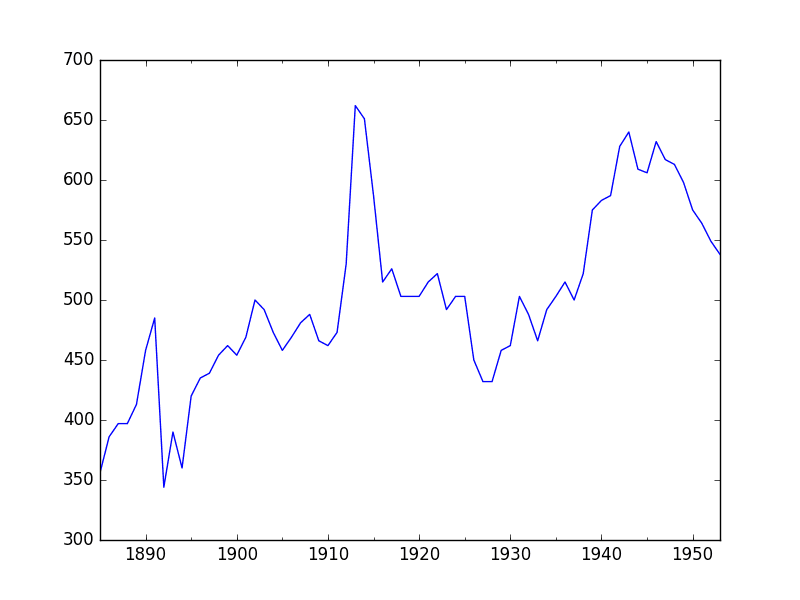
There looks to be an increasing trend in water usage over time.
There do not appear to be any obvious outliers, although there are some large fluctuations.
There is a downward trend for the last few years of the series.
Annual Water Usage Line Plot
There may be some benefit in explicitly modeling the trend component and removing it. You may also explore using differencing with one or two levels in order to make the series stationary.
5.3. Density Plot
Reviewing plots of the density of observations can provide further insight into the structure of the data.
The example below creates a histogram and density plot of the observations without any temporal structure.
1
2
3
4
5
6
7
8
9
from pandas import read_csv
from matplotlib import pyplot
series=read_csv('dataset.csv')
pyplot.figure(1)
pyplot.subplot(211)
series.hist()
pyplot.subplot(212)
series.plot(kind='kde')
pyplot.show()
Run the example and review the plots.
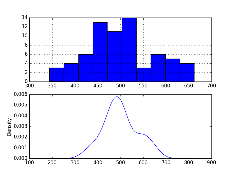
Some observations from the plots include:
The distribution is not Gaussian, but is pretty close.
The distribution has a long right tail and may suggest an exponential distribution or a double Gaussian.
Annual Water Usage Density Plots
This suggests it may be worth exploring some power transforms of the data prior to modeling.
5.4. Box and Whisker Plots
We can group the annual data by decade and get an idea of the spread of observations for each decade and how this may be changing.
We do expect to see some trend (increasing mean or median), but it may be interesting to see how the rest of the distribution may be changing.
The example below groups the observations by decade and creates one box and whisker plot for each decade of observations. The last decade only contains 9 years and may not be a useful comparison with the other decades. Therefore only data between 1885 and 1944 was plotted.
Running the example creates 6 box and whisker plots side-by-side, one for the 6 decades of selected data.
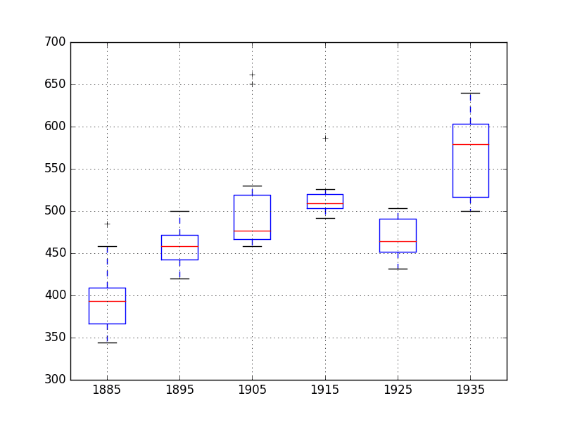
Some observations from reviewing the plot include:
The median values for each year (red line) may show an increasing trend that may not be linear.
The spread, or middle 50% of the data (blue boxes), does show some variability.
There maybe outliers in some decades (crosses outside of the box and whiskers).
The second to last decade seems to have a lower average consumption, perhaps related to the first world war.
Annual Water Usage Box and Whisker Plots
This yearly view of the data is an interesting avenue and could be pursued further by looking at summary statistics from decade-to-decade and changes in summary statistics.
6. ARIMA Models
In this section, we will develop Autoregressive Integrated Moving Average or ARIMA models for the problem.
We will approach modeling by both manual and automatic configuration of the ARIMA model. This will be followed by a third step of investigating the residual errors of the chosen model.
As such, this section is broken down into 3 steps:
Manually Configure the ARIMA.
Automatically Configure the ARIMA.
Review Residual Errors.
6.1 Manually Configured ARIMA
The ARIMA(p,d,q) model requires three parameters and is traditionally configured manually.
Analysis of the time series data assumes that we are working with a stationary time series.
The time series is likely non-stationary. We can make it stationary by first differencing the series and using a statistical test to confirm that the result is stationary.
The example below creates a stationary version of the series and saves it to file stationary.csv.
Running the example outputs the result of a statistical significance test of whether the differenced series is stationary. Specifically, the augmented Dickey-Fuller test.
The results show that the test statistic value -6.126719 is smaller than the critical value at 1% of -3.534. This suggests that we can reject the null hypothesis with a significance level of less than 1% (i.e. a low probability that the result is a statistical fluke).
Rejecting the null hypothesis means that the process has no unit root, and in turn that the time series is stationary or does not have time-dependent structure.
1
2
3
4
5
6
ADF Statistic: -6.126719
p-value: 0.000000
Critical Values:
5%: -2.906
1%: -3.534
10%: -2.591
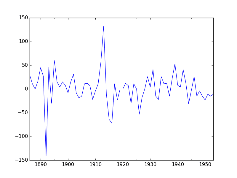
This suggests that at least one level of differencing is required. The d parameter in our ARIMA model should at least be a value of 1.
A plot of the differenced data is also created. It suggests that this has indeed removed the increasing trend.
Differenced Annual Water Usage Dataset
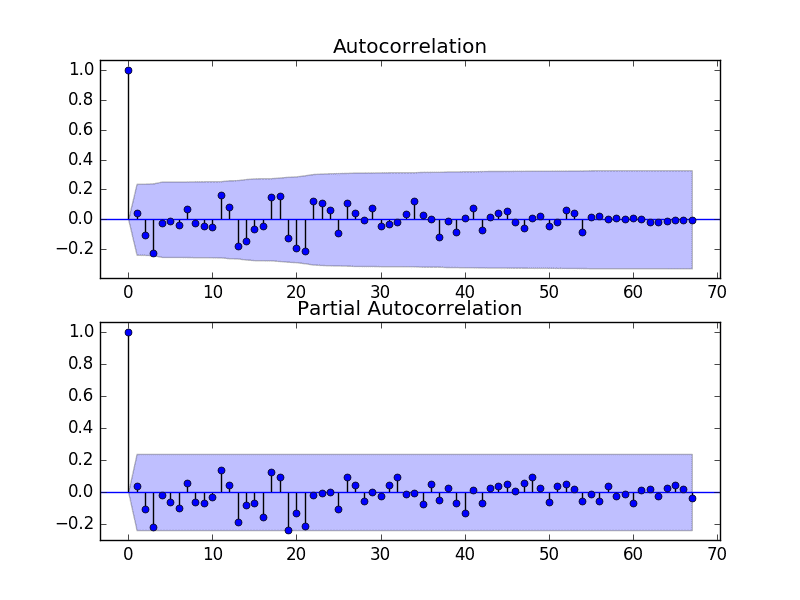
The next first step is to select the lag values for the Autoregression (AR) and Moving Average (MA) parameters, p and q respectively.
We can do this by reviewing Autocorrelation Function (ACF) and Partial Autocorrelation Function (PACF) plots.
The example below creates ACF and PACF plots for the series.
1
2
3
4
5
6
7
8
9
10
11
from pandas import read_csv
from statsmodels.graphics.tsaplots import plot_acf
from statsmodels.graphics.tsaplots import plot_pacf
from matplotlib import pyplot
series=read_csv('dataset.csv')
pyplot.figure()
pyplot.subplot(211)
plot_acf(series,ax=pyplot.gca())
pyplot.subplot(212)
plot_pacf(series,ax=pyplot.gca())
pyplot.show()
Run the example and review the plots for insights into how to set the p and q variables for the ARIMA model.
Below are some observations from the plots.
The ACF shows no significant lags.
The PACF also shows no significant lags.
A good starting point for the p and q values is also 0.
ACF and PACF Plots of Stationary Annual Water Usage Dataset
This quick analysis suggests an ARIMA(0,1,0) on the raw data may be a good starting point.
This is in fact a persistence model. The complete example is listed below.
Running this example results in an RMSE of 22.311, which is slightly higher than the persistence model above.
This may be because of the details of the ARIMA implementation, such as an automatic trend constant that is calculated and added.
1
2
3
4
5
6
7
...
>Predicted=617.079, Expected=598
>Predicted=601.781, Expected=575
>Predicted=578.369, Expected=564
>Predicted=567.152, Expected=549
>Predicted=551.881, Expected=538
RMSE: 22.311
6.2 Grid Search ARIMA Hyperparameters
The ACF and PACF plots suggest that we cannot do better than a persistence model on this dataset.
To confirm this analysis, we can grid search a suite of ARIMA hyperparameters and check that no models result in better out of sample RMSE performance.
In this section, we will search values of p, d, and q for combinations (skipping those that fail to converge), and find the combination that results in the best performance. We will use a grid search to explore all combinations in a subset of integer values.
Specifically, we will search all combinations of the following parameters:
p: 0 to 4.
d: 0 to 2.
q: 0 to 4.
This is (5 * 3 * 5), or 300 potential runs of the test harness, and will take some time to execute.
The complete worked example with the grid search version of the test harness is listed below.
1
2
3
4
5
6
7
8
9
10
11
12
13
14
15
16
17
18
19
20
21
22
23
24
25
26
27
28
29
30
31
32
33
34
35
36
37
38
39
40
41
42
43
44
45
46
47
48
49
50
51
# grid search ARIMA parameters for a time series
import warnings
from pandas import read_csv
from statsmodels.tsa.arima.model import ARIMA
from sklearn.metrics import mean_squared_error
from math import sqrt
# evaluate an ARIMA model for a given order (p,d,q) and return RMSE
def evaluate_arima_model(X,arima_order):
# prepare training dataset
X=X.astype('float32')
train_size=int(len(X)*0.50)
train,test=X[0:train_size],X[train_size:]
history=[xforxintrain]
# make predictions
predictions=list()
fortinrange(len(test)):
model=ARIMA(history,order=arima_order)
model_fit=model.fit()
yhat=model_fit.forecast()[0]
predictions.append(yhat)
history.append(test[t])
# calculate out of sample error
rmse=sqrt(mean_squared_error(test,predictions))
returnrmse
# evaluate combinations of p, d and q values for an ARIMA model
Running the example runs through all combinations and reports the results on those that converge without error. The example takes a little over 2 minutes to run on modern hardware.
The results show that the best configuration discovered was ARIMA(2, 1, 0) with an RMSE of 21.733, slightly lower than the manual persistence model tested earlier, but may or may not be significantly different.
1
2
3
4
5
6
7
...
ARIMA(4, 1, 0) RMSE=24.802
ARIMA(4, 1, 1) RMSE=25.103
ARIMA(4, 2, 0) RMSE=27.089
ARIMA(4, 2, 1) RMSE=25.932
ARIMA(4, 2, 2) RMSE=25.418
Best ARIMA(2, 1, 0) RMSE=21.733
We will select this ARIMA(2, 1, 0) model going forward.
6.3 Review Residual Errors
A good final check of a model is to review residual forecast errors.
Ideally, the distribution of residual errors should be a Gaussian with a zero mean.
We can check this by using summary statistics and plots to investigate the residual errors from the ARIMA(2, 1, 0) model. The example below calculates and summarizes the residual forecast errors.
Running the example first describes the distribution of the residuals.
We can see that the distribution has a right shift and that the mean is non-zero at 1.081624.
This is perhaps a sign that the predictions are biased.
1
2
3
4
5
6
7
8
count 35.000000
mean 1.081624
std 22.022566
min -52.103811
25% -16.202283
50% -0.459801
75% 12.085091
max 51.284336
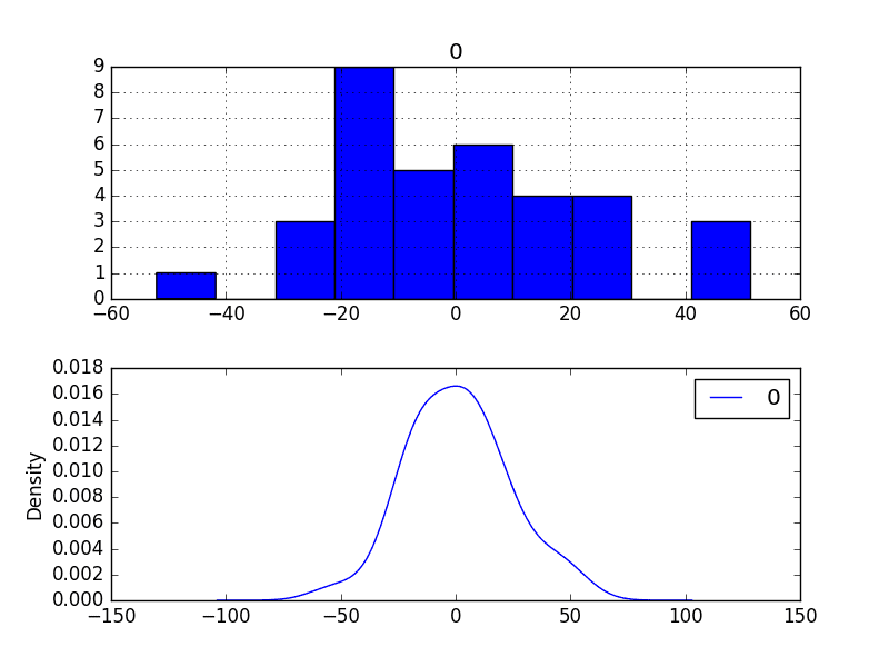
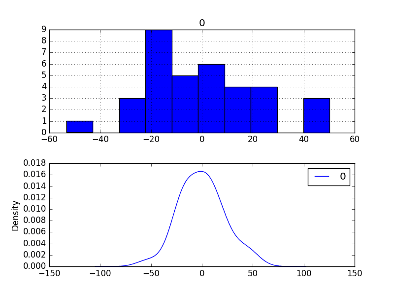
The distribution of residual errors is also plotted.
The graphs suggest a Gaussian-like distribution with a longer right tail, providing further evidence that perhaps a power transform might be worth exploring.
Residual Forecast Errors Density Plots
We could use this information to bias-correct predictions by adding the mean residual error of 1.081624 to each forecast made.
The example below performs this bias-correction.
1
2
3
4
5
6
7
8
9
10
11
12
13
14
15
16
17
18
19
20
21
22
23
24
25
26
27
28
29
30
31
32
33
34
35
36
37
38
39
40
41
# summarize residual errors from bias corrected forecasts
# bias constant, could be calculated from in-sample mean residual
bias=1.081624
# save model
model_fit.save('model.pkl')
numpy.save('model_bias.npy',[bias])
Running the example creates two local files:
model.pkl This is the ARIMAResult object from the call to ARIMA.fit(). This includes the coefficients and all other internal data returned when fitting the model.
model_bias.npy This is the bias value stored as a one-row, one-column NumPy array.
7.2 Make Prediction
A natural case may be to load the model and make a single forecast.
This is relatively straightforward and involves restoring the saved model and the bias and calling the forecast() function.
The example below loads the model, makes a prediction for the next time step, and prints the prediction.
1
2
3
4
5
6
7
# load finalized model and make a prediction
from statsmodels.tsa.arima.model import ARIMAResults
import numpy
model_fit=ARIMAResults.load('model.pkl')
bias=numpy.load('model_bias.npy')
yhat=bias+float(model_fit.forecast()[0])
print('Predicted: %.3f'%yhat)
Running the example prints the prediction of about 540.
1
Predicted: 540.013
If we peek inside validation.csv, we can see that the value on the first row for the next time period is 568. The prediction is in the right ballpark.
7.3 Validate Model
We can load the model and use it in a pretend operational manner.
In the test harness section, we saved the final 10 years of the original dataset in a separate file to validate the final model.
We can load this validation.csv file now and use it to see how well our model really is on “unseen” data.
There are two ways we might proceed:
Load the model and use it to forecast the next 10 years. The forecast beyond the first one or two years will quickly start to degrade in skill.
Load the model and use it in a rolling-forecast manner, updating the transform and model for each time step. This is the preferred method as it is how one would use this model in practice as it would achieve the best performance.
As with model evaluation in the previous sections, we will make predictions in a rolling-forecast manner. This means that we will step over lead times in the validation dataset and take the observations as an update to the history.
1
2
3
4
5
6
7
8
9
10
11
12
13
14
15
16
17
18
19
20
21
22
23
24
25
26
27
28
29
30
31
32
33
34
35
36
37
38
39
40
# load and evaluate the finalized model on the validation dataset
from pandas import read_csv
from matplotlib import pyplot
from statsmodels.tsa.arima.model import ARIMA
from statsmodels.tsa.arima.model import ARIMAResults
Running the example prints each prediction and expected value for the time steps in the validation dataset.
The final RMSE for the validation period is predicted at 16 liters per capita per day. This is not too different from the expected error of 21, but I would expect that it is also not too different from a simple persistence model.
1
2
3
4
5
6
7
8
9
10
11
>Predicted=540.013, Expected=568
>Predicted=571.589, Expected=575
>Predicted=573.289, Expected=579
>Predicted=579.561, Expected=587
>Predicted=588.063, Expected=602
>Predicted=603.022, Expected=594
>Predicted=593.178, Expected=587
>Predicted=588.558, Expected=587
>Predicted=588.797, Expected=625
>Predicted=627.941, Expected=613
RMSE: 16.532
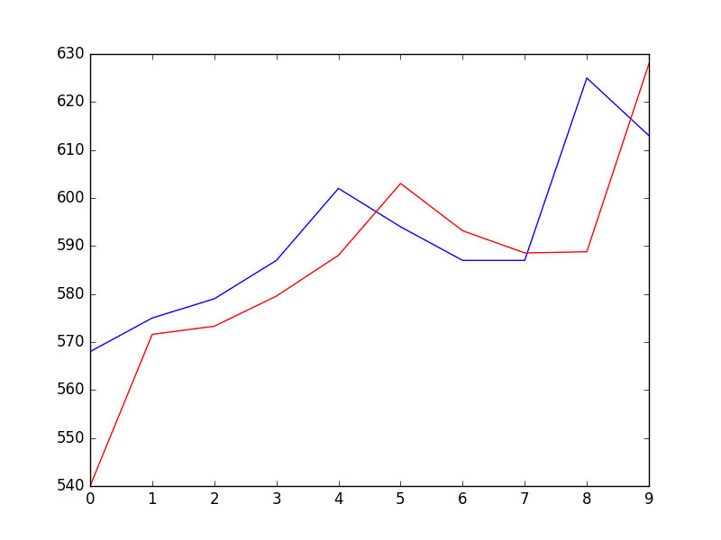
A plot of the predictions compared to the validation dataset is also provided.
The forecast does have the characteristics of a persistence forecast. This suggests that although this time series does have an obvious trend, it is still a reasonably difficult problem.
Plot of Forecast for Validation Dataset
Summary
In this tutorial, you discovered the steps and the tools for a time series forecasting project with Python.
We covered a lot of ground in this tutorial; specifically:
How to develop a test harness with a performance measure and evaluation method and how to quickly develop a baseline forecast and skill.
How to use time series analysis to raise ideas for how to best model the forecast problem.
How to develop an ARIMA model, save it, and later load it to make predictions on new data.
How did you do? Do you have any questions about this tutorial?
Ask your questions in the comments below and I will do my best to answer.
Want to Develop Time Series Forecasts with Python?
1) How to set (p,d,q) by looking at the ACF and PACF plot and auto-correlation plot?
2) How do we know at the beginning if should take first order or second order differences?
3) Below is the result of Dicker-Fuller test on my original data without taking any differences/transformation/moving averages:
And as you can see, since p-value <0.05, I can reject my null hypothesis meaning time series is stationary.. how should I proceed next ?
Test Statistic -3.841070
p-value 0.002514
#Lags Used 1.000000
Number of Observations Used 106.000000
Critical Value (5%) -2.889217
Critical Value (1%) -3.493602
Critical Value (10%) -2.581533
4) how to study residual plots (non-zero mean that you mentioned in your article)?
5) I want to run the code on overall data-set and just use future date values (with no actual value being present) as test set i.e. 1-jan-15,1-Feb-15 etc.. How can I simplify your code to do that ?
5. Train an ARIMA on all of your data, then use the predict() function and it will perform multiple one-step forecasts and use prior forecast values as inputs for the next forecast.
My data is already stationary without even taking any differences as you can see from above results using Dicker Fuller test.
I am still not sure about how do get predictions for future dates.
I trained my data on overall dataset and then tried using predict function to forecast but then predict function has following arguments(start,end,typ,dynamic):
when I try to run my predict function:
model = ARIMA(history, order=(0,1,1))
model_fit = model.fit(disp=0)
model_fit.predict(dates.get_loc(pd.Timestamp(“1-22-2017”)),dates.get_loc(pd.Timestamp(“1-28-2018”)),dynamic=True,typ=’levels’):
it gives me below error saying that “The start index -1 of the original series has been differenced away”. ??
Not sure what you meant by “use prior forecast values as inputs for the next forecast.”
Would really appreciate if you can give an example.
Please note that I am trying to do weekly forecast i.e. I want my start parameter to hold 22-Jan-2017 and end to be 28-Jan-2018 doing forecast for each week with a gap of 7 days
Looking at your ARIMA(0,1,1) you have a difference of 1 in the (the middle part of the order). If your data is stationary, you may not need this (e.g. set d to 0).
I like to use time indexes rather than times in the predict function. Nevertheless, try doing a one step forecast first:
A limitation of this model is that to predict t+2 we must first predict t+1 and use that as an input (lag variable) to predict t+2. This means the forecast skill will likely degrade quickly over future time steps.
So if my data is stationary, then what values of (p,d,q) I should set ?
My ACF/PACF plots cross the zero line before 1st lag, so if everything is 0,0,0 then what type of model(AR/MA/ARIMA/SARIMAX) it is ?
If I use len(history) in start and end parameter, the predict function considers it like an integer values instead of date format and hence the next 7 predictions are very close to each other rather than being different.
With the ACF and PACF plots we are not looking at crossing the zero line, we are looking at autocorrelation that is significant.
If you are unsure of parameters and interpreting ACF and PACF plots, consider using a grid search on the parameters to find the model that has the best out of sample RMSE score.
Re the predict() function, yes I was assuming you wanted the next 7 contiguous time steps, sorry.
So while looking at ACF/PACF plot, I see significant lags at 0 for both of them and my grid search paremeters it selects (1,0,1) as the best model ?
Not sure if I should I take a log or difference of log.
I have the same question again, since I want to do long term forecast say next 12 months or next 52 weeks and I use (p,1,q) model, how do I use predict function to forecast ? It gives me below error
“The start index -1 of the original series has been differenced away”.
My training data has values till 22 Jan 2017 and I am trying to forecast from 29 Jan 2017 upto 28 Jan 2018 so what should my predict function looks like ?
predict(start=?, end= ?, typ=?, dynamic=?)
How can I use t+1 prediction and use that as an input (lag variable) to predict t+2 ?
Let me know if you want me to change my training/test data in a way to accommodate same time period so that I can get rid of differencing error.
Can you please explain it using some sample code using my time periods ?
Great content. Have read your other books. It’s really interesting to read the subject content on your books, well structured and the best way someone can learn from scratch and implement. Eagerly waiting for your Time series Book release.
Anthony from Sydney AustraliaFebruary 21, 2017 at 4:42 pm#
Dear Dr Jason,
Questions please:
(1) From my understanding of the model, you were doing one step ahead predictions every time you updated the history variable. I understand that.
I also understand that instead of the loop, if you predicted 10 steps ahead from the non-updated-version of history, the errors of the predictions would increase as time increases.
In the above listing, what was the purpose of ‘reducing’ the size of the original data and call it ‘train’, and the remainder ‘test’ (size 10) if you are only going to predict one step ahead. Is there something I am missing.
(2) When you use integration variable ‘i’=1 in the ARIMA model, aren’t the predictions differences? For a one step ahead prediction, don’t you have to add model.forecast()[0] to the history[-1] in order to get the predicted value?
Dear Jason,
I had a look at the section 5.4 Box and whisker. I have been experimenting with group = series[‘1885′:’1944′].groupby(TimeGrouper(’10AS’)). I tried variations of TimeGrouper(’10’), TimeGrouper(’10A’) and obtained different results. Don’t try TimeGrouper(’10SA’), otherwise the IDLE program may get stuck.
I generally get the concept of grouping data in groups of 10 years, but cannot find in the pandas documentation TimeGrouper any systematic and consistent parameters to put in the TimeGrouper. For example what is the meaning of ‘A’ and ‘S’ in TimeGrouper(’10AS’).
I like the idea of ‘exploratory data analysis’ to visually inspect the data and the idea of grouping makes me think of the sunspot data. Here’s the question. If this was sunspot data, would TimeGrouper be set as TimeGrouper(’11’) or something else.
Thank you,
Anthony from Sydney Australia
You can even get descriptive statistics of the groups by invoking groups.describe(). However, I was looking at the documentation for TimeGrouper, and there
Are you planning to illustrate how “external variables” as impacting target variable. i.e “water usage” in this case. like temperature, number of people etc.. more than one external variable to be precise.
I have seen ARIMAX and SARIMAX , but no blogs on the same with as much detail as you write up in.
It would be a very helpful for students like me who are trying out different models in quest of knowledge
Hello Jason,
thank you so much for your incredible and informative tutorial, I have a problem when it comes to box and whisker, my dataframe is empty, so I cannot pack the group values into decades, please help me out
This is odd, sorry to hear that Bryan. I have tested the code with Python 2 and 3.
Perhaps confirm that the raw data file is correct and does not contain a footer or extra noise. A bad input file might be the best explanation I can think of.
Thank you for your reply, another thing, I tried to run the stage 6.2 Grid Search ARIMA Hyperparameters on a very large dataset, but it’s very slow, is there a way to speed it up? Thank you very much.
Using your example, I got good results. p,d,q (1,2,0)
These are an extract pedictions and expected values.
>Predicted=11022046.043, Expected=11021346
>Predicted=11379505.273, Expected=11376906
RMSE: 3019.389
My series, dataset, validation are in format Year, Series. (YYYY, Series_value_in_int)
My last year in validation.csv is 2018 and I wish I can predict and plot 5 or 10 years more out of my validation set i.e (2019-2024 or 2019-2030).
What if my three files are in format YYYY-MM-DD as index?
How do I write my code?
Suppose that you continue your example, how would you write your code to predict values for 1964-1974?
Hello Sir,
I tried 7.3 code of yours, but i’m getting the error as cannot convert string to float, i made changes for X = dataset.values.astype(‘float32’) as X=float(dataset()) . Still I’m getting error as ‘Series’ object is not callable. please guide me.
i was unable to run your this page code. But i tried your ARIMA example code.it was successful.Thanks for your tutorial on this. but now how to predict the water usage based on the water level in the sump and the tank. how should i write it in python.
Hi there, a very helpful article indeed. I am wondering the way how a time series model evolve with the time in terms of accuracy of the forecast. Will it automatically improve or does it need a tuning as we do in neural networks. Can you explain this, becuase I can’t find a guidance to this problem.
Hi Jason;
This is really a great tutorial and it was really helpful setting up an ARIMA model.
I have a question regarding the final plot of the rolling ARIMA model under 7.3 for the last ten years.
You said the plot has the characteristics of a naive model which is pretty obvious to me. But what does this imply exactly? That we cannot forecast the water usage accurately? Shouldn’t the ARIMA model outperform the persistence model more clearly?
So, what if ARIMA and the persistence model are nearly the same in terms of accuracy?
Hi Dr Jason, Thanks a lot for sharing your articles.
I need to predict End Time of gas from a cylinder. With provided Time and gas depletion values. gas depletes or replaced by exhaust gases in one feature. Time is given in mins
Can you suggest post to work with the problem.
I was wondering about the line plot that is displayed under section 5.2 which shows (I believe) the consumption patterns vs. the Year values (in x-axis). Using the same codes I could not get the year values though. I am simply getting values of 10, 20… 70.
The only way I could get the year value was by keeing both the year and consumption columns (in the dataset while creating it in section 3.1) and plotting it on the “x” (Year) and “y” (Water) co-ords.
Is there a way I could have the year values in the x-axis with the single columned “dataset” of “Water” consumption data?


")
")
")

Such a great article. many thanks.
Thanks Salem.
Great article Jason!
A couple of questions,
1) How to set (p,d,q) by looking at the ACF and PACF plot and auto-correlation plot?
2) How do we know at the beginning if should take first order or second order differences?
3) Below is the result of Dicker-Fuller test on my original data without taking any differences/transformation/moving averages:
And as you can see, since p-value <0.05, I can reject my null hypothesis meaning time series is stationary.. how should I proceed next ?
Test Statistic -3.841070
p-value 0.002514
#Lags Used 1.000000
Number of Observations Used 106.000000
Critical Value (5%) -2.889217
Critical Value (1%) -3.493602
Critical Value (10%) -2.581533
4) how to study residual plots (non-zero mean that you mentioned in your article)?
5) I want to run the code on overall data-set and just use future date values (with no actual value being present) as test set i.e. 1-jan-15,1-Feb-15 etc.. How can I simplify your code to do that ?
Will really appreciate the help. Thanks!
Hi Kuber, great questions!
1. This post has more on how to configure ARIMA given ACF and PACF plots:
https://machinelearningmastery.com/gentle-introduction-autocorrelation-partial-autocorrelation/
2. If the first order difference does not make the series stationary, repeat until it does.
3. The results suggests that series may be stationary.
4. Learn more about residual plots here:
https://machinelearningmastery.com/visualize-time-series-residual-forecast-errors-with-python/
5. Train an ARIMA on all of your data, then use the predict() function and it will perform multiple one-step forecasts and use prior forecast values as inputs for the next forecast.
I hope that helps.
Hi Jason,
My data is already stationary without even taking any differences as you can see from above results using Dicker Fuller test.
I am still not sure about how do get predictions for future dates.
I trained my data on overall dataset and then tried using predict function to forecast but then predict function has following arguments(start,end,typ,dynamic):
when I try to run my predict function:
model = ARIMA(history, order=(0,1,1))
model_fit = model.fit(disp=0)
model_fit.predict(dates.get_loc(pd.Timestamp(“1-22-2017”)),dates.get_loc(pd.Timestamp(“1-28-2018”)),dynamic=True,typ=’levels’):
it gives me below error saying that “The start index -1 of the original series has been differenced away”. ??
Not sure what you meant by “use prior forecast values as inputs for the next forecast.”
Would really appreciate if you can give an example.
Thanks!
Please note that I am trying to do weekly forecast i.e. I want my start parameter to hold 22-Jan-2017 and end to be 28-Jan-2018 doing forecast for each week with a gap of 7 days
Hi Kuber,
Looking at your ARIMA(0,1,1) you have a difference of 1 in the (the middle part of the order). If your data is stationary, you may not need this (e.g. set d to 0).
I like to use time indexes rather than times in the predict function. Nevertheless, try doing a one step forecast first:
which should be the same as
Then try a longer forecast, such as multiple time steps:
A limitation of this model is that to predict t+2 we must first predict t+1 and use that as an input (lag variable) to predict t+2. This means the forecast skill will likely degrade quickly over future time steps.
Does that help?
Thanks for your reply Jason!
So if my data is stationary, then what values of (p,d,q) I should set ?
My ACF/PACF plots cross the zero line before 1st lag, so if everything is 0,0,0 then what type of model(AR/MA/ARIMA/SARIMAX) it is ?
If I use len(history) in start and end parameter, the predict function considers it like an integer values instead of date format and hence the next 7 predictions are very close to each other rather than being different.
Please let me know.
Hi Kuber,
With the ACF and PACF plots we are not looking at crossing the zero line, we are looking at autocorrelation that is significant.
If you are unsure of parameters and interpreting ACF and PACF plots, consider using a grid search on the parameters to find the model that has the best out of sample RMSE score.
Re the predict() function, yes I was assuming you wanted the next 7 contiguous time steps, sorry.
While looking at ACF/PACF plots I am getting lag values less than 1 i.e. 0.05 and 0.02 for p and q respectively.. Not sure how to proceed ?
Any thoughts ?
Hi Kuber,
Try a grid search of parameters:
https://machinelearningmastery.com/grid-search-arima-hyperparameters-with-python/
Maybe your data is not predictable:
https://machinelearningmastery.com/gentle-introduction-random-walk-times-series-forecasting-python/
Maybe you need a non-linear method or more data?
So while looking at ACF/PACF plot, I see significant lags at 0 for both of them and my grid search paremeters it selects (1,0,1) as the best model ?
Not sure if I should I take a log or difference of log.
Please let me know.
Thanks!
Hi Kuber,
The lag at t=0 can be ignored, it is the correlation of the observation with itself.
The ACF and PACF diagnostics provide a good starting point for a model. You can use grid search to see if you can do better.
A box-cox transform can be good if your data has a changing variance over time. Try it and see.
I have only limited data so getting more data is not an option.
Grid search gives me (1,0,1) as best model , and so as auto.arima() function in R.
One thing I am not sure about is whether to include trend=”c” or “nc”.. what kind of non-linear models should I look into ?
Hi Kuber,
Try with and without the trend (c and nc) and see what works best.
Try a suite of methods, you cannot know what will work best, see this post:
https://machinelearningmastery.com/a-data-driven-approach-to-machine-learning/
Hi Jason,
I have the same question again, since I want to do long term forecast say next 12 months or next 52 weeks and I use (p,1,q) model, how do I use predict function to forecast ? It gives me below error
“The start index -1 of the original series has been differenced away”.
My training data has values till 22 Jan 2017 and I am trying to forecast from 29 Jan 2017 upto 28 Jan 2018 so what should my predict function looks like ?
predict(start=?, end= ?, typ=?, dynamic=?)
How can I use t+1 prediction and use that as an input (lag variable) to predict t+2 ?
Let me know if you want me to change my training/test data in a way to accommodate same time period so that I can get rid of differencing error.
Can you please explain it using some sample code using my time periods ?
Hi Kuber,
With a d=1 it means that your dataset has shrunk by one observation.
This means you need to take this into account when setting start and end.
For example, with d=0 you fit your model with 100 samples (time index 0 to index 99), a one-step forecast would use index 100:
With a d=1, I would expect you are fitting your model on time index 0 to 98 and the one stpe forecast would be:
Try and see, am I right?
If this is all correct, you can scale up to a multi-step forecast.
This makes sense. How about “typ” and “dynamic” parameter in predict function ?
Just not sure what value to set for these parameters for d=0 and d=1 with trend=’c’ and ‘nc’ ?
It would be great if you can fill in below table with typ | dynamic values for each combination. Sorry, but super confused.
trend c nc
d=0 typ | dynamic typ | dynamic
d=1 typ | dynamic typ | dynamic
how above combination affects predict and forecast function ?
Please let me know. Thanks!
Great question.
You can drop typ and dynamic in the predict function. They are not needed.
The c and nc when fitting the model specify whether or not to use a trend constant in the model. Try your model with and without them.
Does that help?
Great content. Have read your other books. It’s really interesting to read the subject content on your books, well structured and the best way someone can learn from scratch and implement. Eagerly waiting for your Time series Book release.
Thanks Debasish.
Dear Dr Jason,
Questions please:
(1) From my understanding of the model, you were doing one step ahead predictions every time you updated the history variable. I understand that.
I also understand that instead of the loop, if you predicted 10 steps ahead from the non-updated-version of history, the errors of the predictions would increase as time increases.
In the above listing, what was the purpose of ‘reducing’ the size of the original data and call it ‘train’, and the remainder ‘test’ (size 10) if you are only going to predict one step ahead. Is there something I am missing.
(2) When you use integration variable ‘i’=1 in the ARIMA model, aren’t the predictions differences? For a one step ahead prediction, don’t you have to add model.forecast()[0] to the history[-1] in order to get the predicted value?
Thank you,
Anthony from Sydney Australia
Hi Anthony, great questions!
1. The idea is to simulate a case where we have unknown data and new observations are available piece-wise.
2. Correct. The forecast() will invert any difference operation, putting forecast values back into their original scale.
Dear Jason,
I had a look at the section 5.4 Box and whisker. I have been experimenting with group = series[‘1885′:’1944′].groupby(TimeGrouper(’10AS’)). I tried variations of TimeGrouper(’10’), TimeGrouper(’10A’) and obtained different results. Don’t try TimeGrouper(’10SA’), otherwise the IDLE program may get stuck.
I generally get the concept of grouping data in groups of 10 years, but cannot find in the pandas documentation TimeGrouper any systematic and consistent parameters to put in the TimeGrouper. For example what is the meaning of ‘A’ and ‘S’ in TimeGrouper(’10AS’).
I like the idea of ‘exploratory data analysis’ to visually inspect the data and the idea of grouping makes me think of the sunspot data. Here’s the question. If this was sunspot data, would TimeGrouper be set as TimeGrouper(’11’) or something else.
Thank you,
Anthony from Sydney Australia
You can even get descriptive statistics of the groups by invoking groups.describe(). However, I was looking at the documentation for TimeGrouper, and there
You can learn about the aliases for grouping here:
http://pandas.pydata.org/pandas-docs/stable/timeseries.html#offset-aliases
Hi Jason,
Are you planning to illustrate how “external variables” as impacting target variable. i.e “water usage” in this case. like temperature, number of people etc.. more than one external variable to be precise.
I have seen ARIMAX and SARIMAX , but no blogs on the same with as much detail as you write up in.
It would be a very helpful for students like me who are trying out different models in quest of knowledge
Thanks for the suggestion Nirikshith. Hopefully in the future.
Hello Jason,
thank you so much for your incredible and informative tutorial, I have a problem when it comes to box and whisker, my dataframe is empty, so I cannot pack the group values into decades, please help me out
I’m sorry to hear that. Does the tutorial example work for you Bryan?
I haven’t finished it yet, I was trying out data analysis to create the box and whisker plot but I keep getting an error. that
decades[name.year] = group.value
I seem to keep getting an error. I think my DataFrame has no value year.
N.B I am using python 2.7 can that be the case?
This is odd, sorry to hear that Bryan. I have tested the code with Python 2 and 3.
Perhaps confirm that the raw data file is correct and does not contain a footer or extra noise. A bad input file might be the best explanation I can think of.
Hi Jason,
I really liked how you explained everything. Looking forward to learn more from other posts.
Thank you very much for making our life easy.
Do you plan to do something on the statistical side of algo’s. Basically how to interpret various things like chi-square, F values etc.
I may in the future if there is a lot of interest.
Hi, Jason, nice blog. Please, can you tell me how to put the date on the x-axis in the chart at the stage 7.3 Validate model? Thank you
You can learn more about the matplotlib API here:
https://matplotlib.org/index.html
Thank you for your reply, another thing, I tried to run the stage 6.2 Grid Search ARIMA Hyperparameters on a very large dataset, but it’s very slow, is there a way to speed it up? Thank you very much.
Bigger machine, or split up the grid search across multiple machines?
Ah ok, I see there isn’t a programmatically solution. Thank you so much
Perhaps a more efficient search procedure, e.g. Bayesian optimization.
Hi Jeson, sorry to bother you! In general, I saw that SARIMAX is faster than ARIMA, can I replace SARIMAX in place of ARIMA? Thank you very much
Really? I found SARIMAX much slower than ARIMA.
Yes, you can use SARIAMX to build an ARIMA. Just set the seasonality arguments to 0.
Using your example, I got good results. p,d,q (1,2,0)
These are an extract pedictions and expected values.
>Predicted=11022046.043, Expected=11021346
>Predicted=11379505.273, Expected=11376906
RMSE: 3019.389
My series, dataset, validation are in format Year, Series. (YYYY, Series_value_in_int)
My last year in validation.csv is 2018 and I wish I can predict and plot 5 or 10 years more out of my validation set i.e (2019-2024 or 2019-2030).
What if my three files are in format YYYY-MM-DD as index?
How do I write my code?
Suppose that you continue your example, how would you write your code to predict values for 1964-1974?
Thanks
Perhaps this post will help for making out of sample predictions:
https://machinelearningmastery.com/make-sample-forecasts-arima-python/
Hello sir,
can u plz send the dataset in the form of .csv file ????reply asap
You can download the dataset from the link.
Also, all datasets are available here:
https://github.com/jbrownlee/Datasets
Yes, here:
https://raw.githubusercontent.com/jbrownlee/Datasets/master/yearly-water-usage.csv
I don’t follow, what do you mean exactly?
The tutorial is about annual water usage and I wrote and ran the tutorial.
Hello sir,
how did you splitted dataset.csv and validation.csv ???
You can split based on a specific year or month.
If you need help working with numpy arrays, perhaps start here:
https://machinelearningmastery.com/index-slice-reshape-numpy-arrays-machine-learning-python/
Hello Sir,
I tried 7.3 code of yours, but i’m getting the error as cannot convert string to float, i made changes for X = dataset.values.astype(‘float32’) as X=float(dataset()) . Still I’m getting error as ‘Series’ object is not callable. please guide me.
Thanks and regards
Bindu TR
Sorry to hear that, I have some suggestions here:
https://machinelearningmastery.com/faq/single-faq/why-does-the-code-in-the-tutorial-not-work-for-me
Hello sir,
will this 7.3 code run on the jupyter notebook??
if yes, It showing the error as ‘cannot convert string to float’ please help me
I suspect it will, but I recommend running from the command line:
https://machinelearningmastery.com/faq/single-faq/how-do-i-run-a-script-from-the-command-line
Hello sir,
As you said, i had run the program in Command prompt of windows, getting the same error as ‘cannot covert string to float values’.help me out
Thanks and Regards
Bindu TR
Perhaps there is an issue with your data file, perhaps try this data file:
https://raw.githubusercontent.com/jbrownlee/Datasets/master/yearly-water-usage.csv
Hello Sir,
I checked everything, I’m unable to run the 7.3 code. i think Series support columns and its not taking row values.
Thanks & Regards
Bindu TR
Sorry to hear that, I believe the code works.
Perhaps double check your environment/libraries/python are up to date?
Hello sir,
i was unable to run your this page code. But i tried your ARIMA example code.it was successful.Thanks for your tutorial on this. but now how to predict the water usage based on the water level in the sump and the tank. how should i write it in python.
Thanks and Regards
bindu TR
This might help:
https://machinelearningmastery.com/make-sample-forecasts-arima-python/
Hi there, a very helpful article indeed. I am wondering the way how a time series model evolve with the time in terms of accuracy of the forecast. Will it automatically improve or does it need a tuning as we do in neural networks. Can you explain this, becuase I can’t find a guidance to this problem.
Thank you, Regards.
Tharika
The model may need to be updated if error in predictions begins to increase.
Thank you Jason 🙂
You’re welcome.
Hi Jason;
This is really a great tutorial and it was really helpful setting up an ARIMA model.
I have a question regarding the final plot of the rolling ARIMA model under 7.3 for the last ten years.
You said the plot has the characteristics of a naive model which is pretty obvious to me. But what does this imply exactly? That we cannot forecast the water usage accurately? Shouldn’t the ARIMA model outperform the persistence model more clearly?
So, what if ARIMA and the persistence model are nearly the same in terms of accuracy?
If the ARIMA cannot do better than a naive forecast, even after we tune the model, it suggest’s ARIMA is not appropriate for the data.
If we get the same finding from many model types, and the best we can do is persistence, it may suggest that the series is not predictable (as-is).
I see. Thanks a lot!
Hi Dr Jason, Thanks a lot for sharing your articles.
I need to predict End Time of gas from a cylinder. With provided Time and gas depletion values. gas depletes or replaced by exhaust gases in one feature. Time is given in mins
Can you suggest post to work with the problem.
Perhaps you can model it as a time series classification task?
This might be a good place to start:
https://machinelearningmastery.com/start-here/#deep_learning_time_series
Hello! I got the RMSE on validation set much higher than on the test set. What does it mean?
It could be a few things:
Perhaps you have overfit the training set?
Perhaps the validation set is very different from the training set?
print(‘>Predicted=%.3f, Expected=%.3f’ % (yhat, y[0]))
TypeError: only size-1 arrays can be converted to Python scalars
what shuld I do ? please help me.
Hello linfeng…did you copy and paste the code? That may be part of the issue.
Dear Jason,
I was wondering about the line plot that is displayed under section 5.2 which shows (I believe) the consumption patterns vs. the Year values (in x-axis). Using the same codes I could not get the year values though. I am simply getting values of 10, 20… 70.
The only way I could get the year value was by keeing both the year and consumption columns (in the dataset while creating it in section 3.1) and plotting it on the “x” (Year) and “y” (Water) co-ords.
Is there a way I could have the year values in the x-axis with the single columned “dataset” of “Water” consumption data?
Best ragrads
I am getting the results printed in the console, but when the script reaches the plot stage, I am getting error:
“TypeError: no numeric data to plot” on line:
“stationary.plot()”
I have copied your codes using the “Copy” menu item in the code widget.
Can you help?