Time series forecasting is a process, and the only way to get good forecasts is to practice this process.
In this tutorial, you will discover how to forecast the monthly sales of French champagne with Python.
Working through this tutorial will provide you with a framework for the steps and the tools for working through your own time series forecasting problems.
After completing this tutorial, you will know:
How to confirm your Python environment and carefully define a time series forecasting problem.
How to create a test harness for evaluating models, develop a baseline forecast, and better understand your problem with the tools of time series analysis.
How to develop an autoregressive integrated moving average model, save it to file, and later load it to make predictions for new time steps.
Kick-start your project with my new book Time Series Forecasting With Python, including step-by-step tutorials and the Python source code files for all examples.
Let’s get started.
Updated Mar/2017: Fixed a typo in the code example.
Updated Apr/2019: Updated the link to dataset.
Updated Aug/2019: Updated data loading and date grouping to use new API.
Updated Feb/2020: Updated to_csv() to remove warnings.
Updated Feb/2020: Fixed data preparation and loading.
Updated May/2020: Fixed small typo when making a prediction.
Updated Dec/2020: Updated modeling for changes to the API.
Time Series Forecast Study with Python – Monthly Sales of French Champagne Photo by Basheer Tome, some rights reserved.
Overview
In this tutorial, we will work through a time series forecasting project from end-to-end, from downloading the dataset and defining the problem to training a final model and making predictions.
This project is not exhaustive, but shows how you can get good results quickly by working through a time series forecasting problem systematically.
The steps of this project that we will through are as follows.
Environment.
Problem Description.
Test Harness.
Persistence.
Data Analysis.
ARIMA Models.
Model Validation.
This will provide a template for working through a time series prediction problem that you can use on your own dataset.
Stop learning Time Series Forecasting the slow way!
Take my free 7-day email course and discover how to get started (with sample code).
Click to sign-up and also get a free PDF Ebook version of the course.
1. Environment
This tutorial assumes an installed and working SciPy environment and dependencies, including:
SciPy
NumPy
Matplotlib
Pandas
scikit-learn
statsmodels
If you need help installing Python and the SciPy environment on your workstation, consider the Anaconda distribution that manages much of it for you.
This script will help you check your installed versions of these libraries.
1
2
3
4
5
6
7
8
9
10
11
12
13
14
15
16
17
18
19
# check the versions of key python libraries
# scipy
import scipy
print('scipy: %s'%scipy.__version__)
# numpy
import numpy
print('numpy: %s'%numpy.__version__)
# matplotlib
import matplotlib
print('matplotlib: %s'%matplotlib.__version__)
# pandas
import pandas
print('pandas: %s'%pandas.__version__)
# statsmodels
import statsmodels
print('statsmodels: %s'%statsmodels.__version__)
# scikit-learn
import sklearn
print('sklearn: %s'%sklearn.__version__)
The results on my workstation used to write this tutorial are as follows:
1
2
3
4
5
6
scipy: 1.5.4
numpy: 1.18.5
matplotlib: 3.3.3
pandas: 1.1.4
statsmodels: 0.12.1
sklearn: 0.23.2
2. Problem Description
The problem is to predict the number of monthly sales of champagne for the Perrin Freres label (named for a region in France).
The dataset provides the number of monthly sales of champagne from January 1964 to September 1972, or just under 10 years of data.
The values are a count of millions of sales and there are 105 observations.
The dataset is credited to Makridakis and Wheelwright, 1989.
Download the dataset as a CSV file and place it in your current working directory with the filename “champagne.csv“.
3. Test Harness
We must develop a test harness to investigate the data and evaluate candidate models.
This involves two steps:
Defining a Validation Dataset.
Developing a Method for Model Evaluation.
3.1 Validation Dataset
The dataset is not current. This means that we cannot easily collect updated data to validate the model.
Therefore we will pretend that it is September 1971 and withhold the last one year of data from analysis and model selection.
This final year of data will be used to validate the final model.
The code below will load the dataset as a Pandas Series and split into two, one for model development (dataset.csv) and the other for validation (validation.csv).
Running the example creates two files and prints the number of observations in each.
1
Dataset 93, Validation 12
The specific contents of these files are:
dataset.csv: Observations from January 1964 to September 1971 (93 observations)
validation.csv: Observations from October 1971 to September 1972 (12 observations)
The validation dataset is about 11% of the original dataset.
Note that the saved datasets do not have a header line, therefore we do not need to cater for this when working with these files later.
3.2. Model Evaluation
Model evaluation will only be performed on the data in dataset.csv prepared in the previous section.
Model evaluation involves two elements:
Performance Measure.
Test Strategy.
3.2.1 Performance Measure
The observations are a count of champagne sales in millions of units.
We will evaluate the performance of predictions using the root mean squared error (RMSE). This will give more weight to predictions that are grossly wrong and will have the same units as the original data.
Any transforms to the data must be reversed before the RMSE is calculated and reported to make the performance between different methods directly comparable.
We can calculate the RMSE using the helper function from the scikit-learn library mean_squared_error() that calculates the mean squared error between a list of expected values (the test set) and the list of predictions. We can then take the square root of this value to give us an RMSE score.
For example:
1
2
3
4
5
6
7
8
from sklearn.metrics import mean_squared_error
from math import sqrt
...
test=...
predictions=...
mse=mean_squared_error(test,predictions)
rmse=sqrt(mse)
print('RMSE: %.3f'%rmse)
3.2.2 Test Strategy
Candidate models will be evaluated using walk-forward validation.
This is because a rolling-forecast type model is required from the problem definition. This is where one-step forecasts are needed given all available data.
The walk-forward validation will work as follows:
The first 50% of the dataset will be held back to train the model.
The remaining 50% of the dataset will be iterated and test the model.
For each step in the test dataset:
A model will be trained.
A one-step prediction made and the prediction stored for later evaluation.
The actual observation from the test dataset will be added to the training dataset for the next iteration.
The predictions made during the iteration of the test dataset will be evaluated and an RMSE score reported.
Given the small size of the data, we will allow a model to be re-trained given all available data prior to each prediction.
We can write the code for the test harness using simple NumPy and Python code.
Firstly, we can split the dataset into train and test sets directly. We’re careful to always convert a loaded dataset to float32 in case the loaded data still has some String or Integer data types.
1
2
3
4
5
# prepare data
X=series.values
X=X.astype('float32')
train_size=int(len(X)*0.50)
train,test=X[0:train_size],X[train_size:]
Next, we can iterate over the time steps in the test dataset. The train dataset is stored in a Python list as we need to easily append a new observation each iteration and NumPy array concatenation feels like overkill.
The prediction made by the model is called yhat for convention, as the outcome or observation is referred to as y and yhat (a ‘y‘ with a mark above) is the mathematical notation for the prediction of the y variable.
The prediction and observation are printed each observation for a sanity check prediction in case there are issues with the model.
The first step before getting bogged down in data analysis and modeling is to establish a baseline of performance.
This will provide both a template for evaluating models using the proposed test harness and a performance measure by which all more elaborate predictive models can be compared.
The baseline prediction for time series forecasting is called the naive forecast, or persistence.
This is where the observation from the previous time step is used as the prediction for the observation at the next time step.
We can plug this directly into the test harness defined in the previous section.
Running the test harness prints the prediction and observation for each iteration of the test dataset.
The example ends by printing the RMSE for the model.
In this case, we can see that the persistence model achieved an RMSE of 3186.501. This means that on average, the model was wrong by about 3,186 million sales for each prediction made.
1
2
3
4
5
6
7
...
>Predicted=4676.000, Expected=5010
>Predicted=5010.000, Expected=4874
>Predicted=4874.000, Expected=4633
>Predicted=4633.000, Expected=1659
>Predicted=1659.000, Expected=5951
RMSE: 3186.501
We now have a baseline prediction method and performance; now we can start digging into our data.
5. Data Analysis
We can use summary statistics and plots of the data to quickly learn more about the structure of the prediction problem.
In this section, we will look at the data from five perspectives:
Summary Statistics.
Line Plot.
Seasonal Line Plots
Density Plots.
Box and Whisker Plot.
5.1 Summary Statistics
Summary statistics provide a quick look at the limits of observed values. It can help to get a quick idea of what we are working with.
The example below calculates and prints summary statistics for the time series.
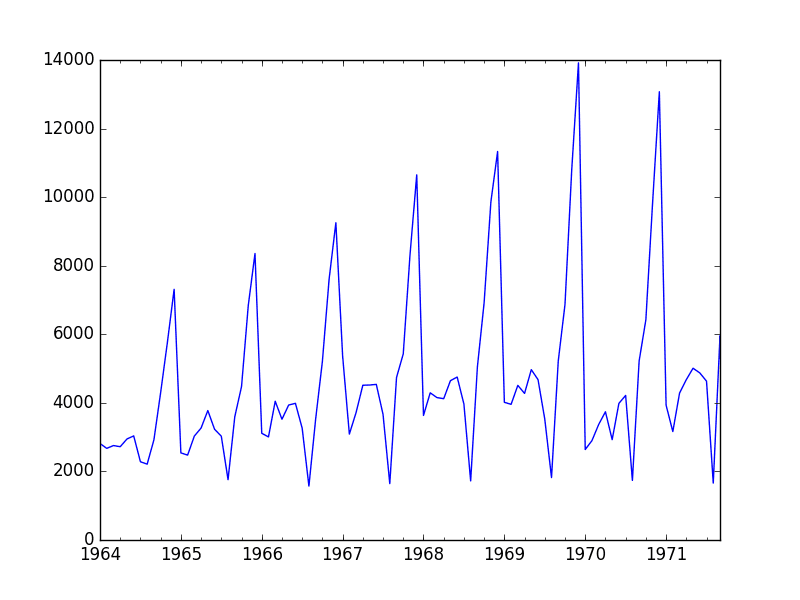
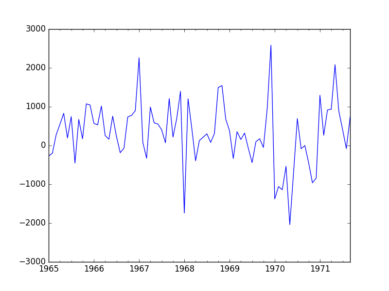
Run the example and review the plot. Note any obvious temporal structures in the series.
Some observations from the plot include:
There may be an increasing trend of sales over time.
There appears to be systematic seasonality to the sales for each year.
The seasonal signal appears to be growing over time, suggesting a multiplicative relationship (increasing change).
There do not appear to be any obvious outliers.
The seasonality suggests that the series is almost certainly non-stationary.
Champagne Sales Line Plot
There may be benefit in explicitly modeling the seasonal component and removing it. You may also explore using differencing with one or two levels in order to make the series stationary.
The increasing trend or growth in the seasonal component may suggest the use of a log or other power transform.
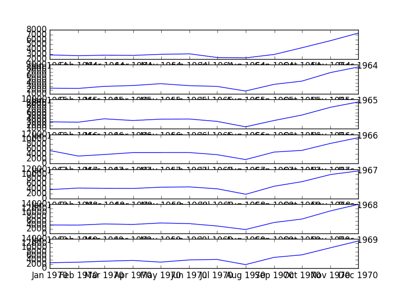
5.3 Seasonal Line Plots
We can confirm the assumption that the seasonality is a yearly cycle by eyeballing line plots of the dataset by year.
The example below takes the 7 full years of data as separate groups and creates one line plot for each. The line plots are aligned vertically to help spot any year-to-year pattern.
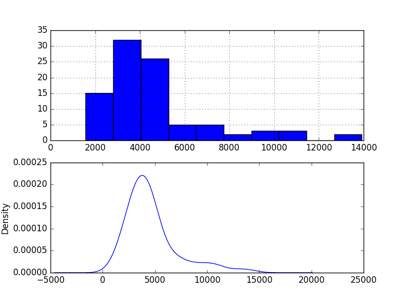
The shape has a long right tail and may suggest an exponential distribution
This lends more support to exploring some power transforms of the data prior to modeling.
5.5 Box and Whisker Plots
We can group the monthly data by year and get an idea of the spread of observations for each year and how this may be changing.
We do expect to see some trend (increasing mean or median), but it may be interesting to see how the rest of the distribution may be changing.
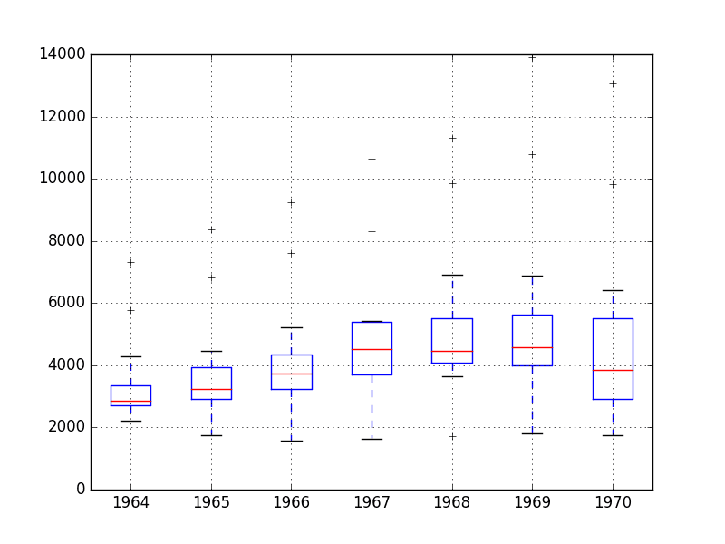
The example below groups the observations by year and creates one box and whisker plot for each year of observations. The last year (1971) only contains 9 months and may not be a useful comparison with the 12 months of observations for other years. Therefore, only data between 1964 and 1970 was plotted.
Running the example creates 7 box and whisker plots side-by-side, one for each of the 7 years of selected data.
Some observations from reviewing the plots include:
The median values for each year (red line) may show an increasing trend.
The spread or middle 50% of the data (blue boxes) does appear reasonably stable.
There are outliers each year (black crosses); these may be the tops or bottoms of the seasonal cycle.
The last year, 1970, does look different from the trend in prior years
Champagne Sales Box and Whisker Plots
The observations suggest perhaps some growth trend over the years and outliers that may be a part of the seasonal cycle.
This yearly view of the data is an interesting avenue and could be pursued further by looking at summary statistics from year-to-year and changes in summary stats from year-to-year.
6. ARIMA Models
In this section, we will develop Autoregressive Integrated Moving Average, or ARIMA, models for the problem.
We will approach modeling by both manual and automatic configuration of the ARIMA model. This will be followed by a third step of investigating the residual errors of the chosen model.
As such, this section is broken down into 3 steps:
Manually Configure the ARIMA.
Automatically Configure the ARIMA.
Review Residual Errors.
6.1 Manually Configured ARIMA
The ARIMA(p,d,q) model requires three parameters and is traditionally configured manually.
Analysis of the time series data assumes that we are working with a stationary time series.
The time series is almost certainly non-stationary. We can make it stationary this by first differencing the series and using a statistical test to confirm that the result is stationary.
The seasonality in the series is seemingly year-to-year. Seasonal data can be differenced by subtracting the observation from the same time in the previous cycle, in this case the same month in the previous year. This does mean that we will lose the first year of observations as there is no prior year to difference with.
The example below creates a deseasonalized version of the series and saves it to file stationary.csv.
Running the example outputs the result of a statistical significance test of whether the differenced series is stationary. Specifically, the augmented Dickey-Fuller test.
The results show that the test statistic value -7.134898 is smaller than the critical value at 1% of -3.515. This suggests that we can reject the null hypothesis with a significance level of less than 1% (i.e. a low probability that the result is a statistical fluke).
Rejecting the null hypothesis means that the process has no unit root, and in turn that the time series is stationary or does not have time-dependent structure.
1
2
3
4
5
6
ADF Statistic: -7.134898
p-value: 0.000000
Critical Values:
5%: -2.898
1%: -3.515
10%: -2.586
For reference, the seasonal difference operation can be inverted by adding the observation for the same month the year before. This is needed in the case that predictions are made by a model fit on seasonally differenced data. The function to invert the seasonal difference operation is listed below for completeness.
1
2
3
# invert differenced value
def inverse_difference(history,yhat,interval=1):
returnyhat+history[-interval]
A plot of the differenced dataset is also created.
The plot does not show any obvious seasonality or trend, suggesting the seasonally differenced dataset is a good starting point for modeling.
We will use this dataset as an input to the ARIMA model. It also suggests that no further differencing may be required, and that the d parameter may be set to 0.
Seasonal Differenced Champagne Sales Line Plot
The next first step is to select the lag values for the Autoregression (AR) and Moving Average (MA) parameters, p and q respectively.
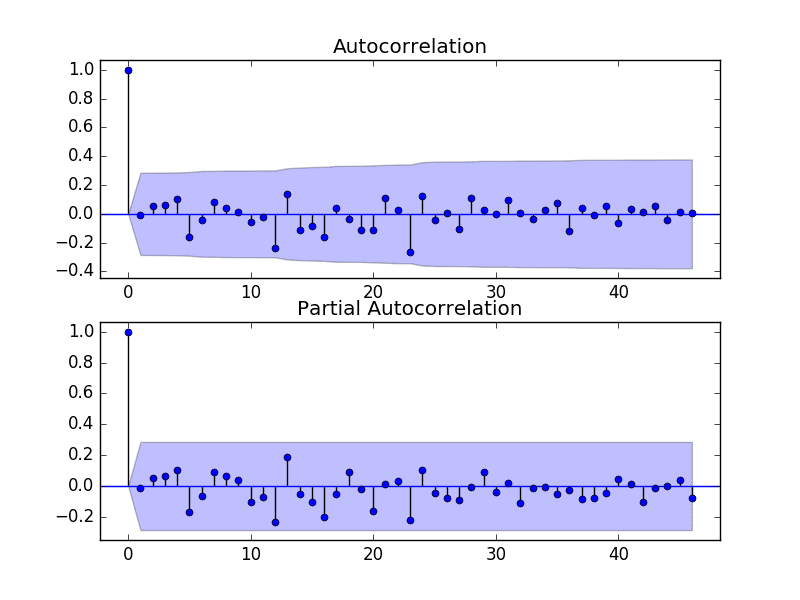
We can do this by reviewing Autocorrelation Function (ACF) and Partial Autocorrelation Function (PACF) plots.
Note, we are now using the seasonally differenced stationary.csv as our dataset.
The example below creates ACF and PACF plots for the series.
1
2
3
4
5
6
7
8
9
10
11
from pandas import read_csv
from statsmodels.graphics.tsaplots import plot_acf
from statsmodels.graphics.tsaplots import plot_pacf
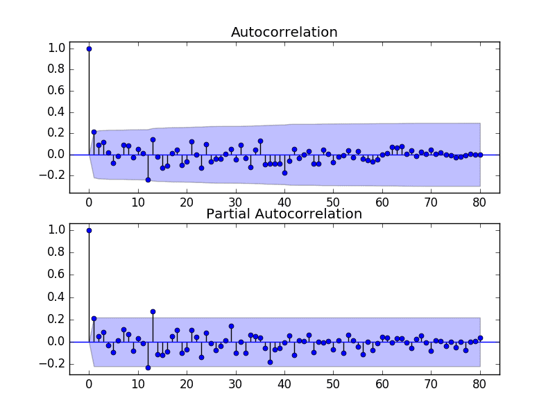
Run the example and review the plots for insights into how to set the p and q variables for the ARIMA model.
Below are some observations from the plots.
The ACF shows a significant lag for 1 month.
The PACF shows a significant lag for 1 month, with perhaps some significant lag at 12 and 13 months.
Both the ACF and PACF show a drop-off at the same point, perhaps suggesting a mix of AR and MA.
A good starting point for the p and q values is also 1.
The PACF plot also suggests that there is still some seasonality present in the differenced data.
We may consider a better model of seasonality, such as modeling it directly and explicitly removing it from the model rather than seasonal differencing.
ACF and PACF Plots of Seasonally Differenced Champagne Sales
This quick analysis suggests an ARIMA(1,0,1) on the stationary data may be a good starting point.
The historic observations will be seasonally differenced prior to the fitting of each ARIMA model. The differencing will be inverted for all predictions made to make them directly comparable to the expected observation in the original sale count units.
Experimentation shows that this configuration of ARIMA does not converge and results in errors by the underlying library. Further experimentation showed that adding one level of differencing to the stationary data made the model more stable. The model can be extended to ARIMA(1,1,1).
We will also disable the automatic addition of a trend constant from the model by setting the ‘trend‘ argument to ‘nc‘ for no constant in the call to fit(). From experimentation, I find that this can result in better forecast performance on some problems.
The example below demonstrates the performance of this ARIMA model on the test harness.
Note, you may see a warning message from the underlying linear algebra library; this can be ignored for now.
Running this example results in an RMSE of 956.942, which is dramatically better than the persistence RMSE of 3186.501.
1
2
3
4
5
6
7
...
>Predicted=3157.018, Expected=5010
>Predicted=4615.082, Expected=4874
>Predicted=4624.998, Expected=4633
>Predicted=2044.097, Expected=1659
>Predicted=5404.428, Expected=5951
RMSE: 956.942
This is a great start, but we may be able to get improved results with a better configured ARIMA model.
6.2 Grid Search ARIMA Hyperparameters
The ACF and PACF plots suggest that an ARIMA(1,0,1) or similar may be the best that we can do.
To confirm this analysis, we can grid search a suite of ARIMA hyperparameters and check that no models result in better out of sample RMSE performance.
In this section, we will search values of p, d, and q for combinations (skipping those that fail to converge), and find the combination that results in the best performance on the test set. We will use a grid search to explore all combinations in a subset of integer values.
Specifically, we will search all combinations of the following parameters:
p: 0 to 6.
d: 0 to 2.
q: 0 to 6.
This is (7 * 3 * 7), or 147, potential runs of the test harness and will take some time to execute.
It may be interesting to evaluate MA models with a lag of 12 or 13 as were noticed as potentially interesting from reviewing the ACF and PACF plots. Experimentation suggested that these models may not be stable, resulting in errors in the underlying mathematical libraries.
The complete worked example with the grid search version of the test harness is listed below.
1
2
3
4
5
6
7
8
9
10
11
12
13
14
15
16
17
18
19
20
21
22
23
24
25
26
27
28
29
30
31
32
33
34
35
36
37
38
39
40
41
42
43
44
45
46
47
48
49
50
51
52
53
54
55
56
57
58
59
60
61
62
63
64
65
66
67
68
# grid search ARIMA parameters for time series
import warnings
from pandas import read_csv
from statsmodels.tsa.arima.model import ARIMA
from sklearn.metrics import mean_squared_error
from math import sqrt
import numpy
# create a differenced series
def difference(dataset,interval=1):
diff=list()
foriinrange(interval,len(dataset)):
value=dataset[i]-dataset[i-interval]
diff.append(value)
returnnumpy.array(diff)
# invert differenced value
def inverse_difference(history,yhat,interval=1):
returnyhat+history[-interval]
# evaluate an ARIMA model for a given order (p,d,q) and return RMSE
Running the example runs through all combinations and reports the results on those that converge without error. The example takes a little over 2 minutes to run on modern hardware.
The results show that the best configuration discovered was ARIMA(0, 0, 1) with an RMSE of 939.464, slightly lower than the manually configured ARIMA from the previous section. This difference may or may not be statistically significant.
1
2
3
4
5
6
7
...
ARIMA(5, 1, 2) RMSE=1003.200
ARIMA(5, 2, 1) RMSE=1053.728
ARIMA(6, 0, 0) RMSE=996.466
ARIMA(6, 1, 0) RMSE=1018.211
ARIMA(6, 1, 1) RMSE=1023.762
Best ARIMA(0, 0, 1) RMSE=939.464
We will select this ARIMA(0, 0, 1) model going forward.
6.3 Review Residual Errors
A good final check of a model is to review residual forecast errors.
Ideally, the distribution of residual errors should be a Gaussian with a zero mean.
We can check this by using summary statistics and plots to investigate the residual errors from the ARIMA(0, 0, 1) model. The example below calculates and summarizes the residual forecast errors.
Running the example first describes the distribution of the residuals.
We can see that the distribution has a right shift and that the mean is non-zero at 165.904728.
This is perhaps a sign that the predictions are biased.
1
2
3
4
5
6
7
8
count 47.000000
mean 165.904728
std 934.696199
min -2164.247449
25% -289.651596
50% 191.759548
75% 732.992187
max 2367.304748
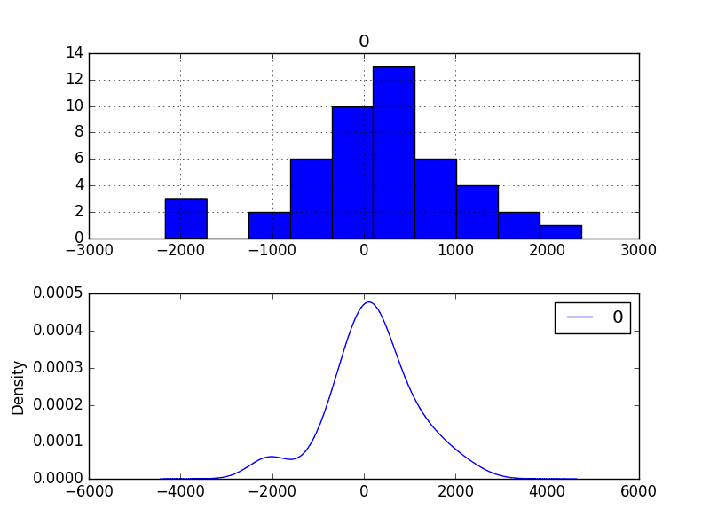
The distribution of residual errors is also plotted.
The graphs suggest a Gaussian-like distribution with a bumpy left tail, providing further evidence that perhaps a power transform might be worth exploring.
Residual Forecast Error Density Plots
We could use this information to bias-correct predictions by adding the mean residual error of 165.904728 to each forecast made.
The example below performs this bias correlation.
1
2
3
4
5
6
7
8
9
10
11
12
13
14
15
16
17
18
19
20
21
22
23
24
25
26
27
28
29
30
31
32
33
34
35
36
37
38
39
40
41
42
43
44
45
46
47
48
49
50
51
52
53
54
55
56
57
58
# plots of residual errors of bias corrected forecasts
The performance of the predictions is improved very slightly from 939.464 to 924.699, which may or may not be significant.
The summary of the forecast residual errors shows that the mean was indeed moved to a value very close to zero.
1
2
3
4
5
6
7
8
9
10
RMSE: 924.699
count 4.700000e+01
mean 4.965016e-07
std 9.346962e+02
min -2.330152e+03
25% -4.555563e+02
50% 2.585482e+01
75% 5.670875e+02
max 2.201400e+03
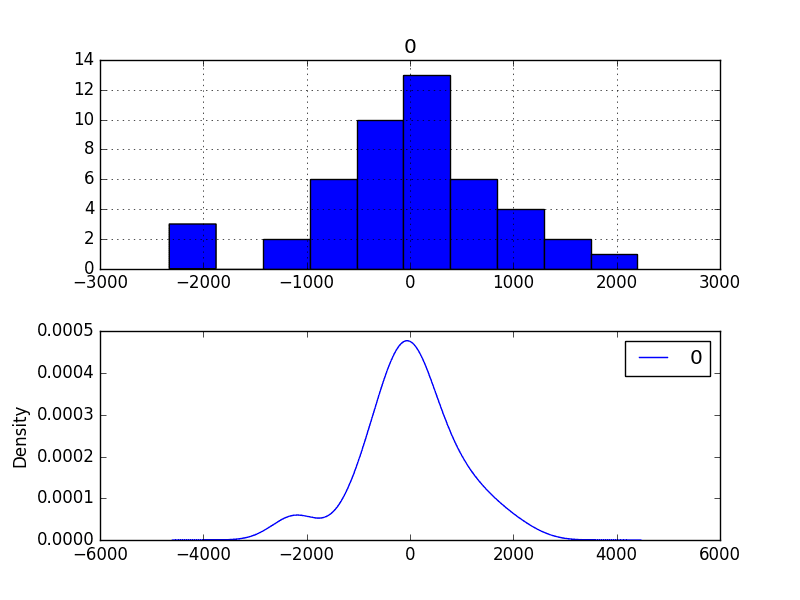
Finally, density plots of the residual error do show a small shift towards zero.
It is debatable whether this bias correction is worth it, but we will use it for now.
Bias-Corrected Residual Forecast Error Density Plots
It is also a good idea to check the time series of the residual errors for any type of autocorrelation. If present, it would suggest that the model has more opportunity to model the temporal structure in the data.
The example below re-calculates the residual errors and creates ACF and PACF plots to check for any significant autocorrelation.
1
2
3
4
5
6
7
8
9
10
11
12
13
14
15
16
17
18
19
20
21
22
23
24
25
26
27
28
29
30
31
32
33
34
35
36
37
38
39
40
41
42
43
44
45
46
47
48
49
50
51
52
53
54
# ACF and PACF plots of residual errors of bias corrected forecasts
from pandas import read_csv
from pandas import DataFrame
from statsmodels.tsa.arima.model import ARIMA
from matplotlib import pyplot
from statsmodels.graphics.tsaplots import plot_acf
from statsmodels.graphics.tsaplots import plot_pacf
# bias constant, could be calculated from in-sample mean residual
bias=165.904728
# save model
model_fit.save('model.pkl')
numpy.save('model_bias.npy',[bias])
Running the example creates two local files:
model.pkl This is the ARIMAResult object from the call to ARIMA.fit(). This includes the coefficients and all other internal data returned when fitting the model.
model_bias.npy This is the bias value stored as a one-row, one-column NumPy array.
7.2 Make Prediction
A natural case may be to load the model and make a single forecast.
This is relatively straightforward and involves restoring the saved model and the bias and calling the forecast() method. To invert the seasonal differencing, the historical data must also be loaded.
The example below loads the model, makes a prediction for the next time step, and prints the prediction.
1
2
3
4
5
6
7
8
9
10
11
12
13
14
15
16
# load finalized model and make a prediction
from pandas import read_csv
from statsmodels.tsa.arima.model import ARIMAResults
Running the example prints the prediction of about 6794.
1
Predicted: 6794.773
If we peek inside validation.csv, we can see that the value on the first row for the next time period is 6981.
The prediction is in the right ballpark.
7.3 Validate Model
We can load the model and use it in a pretend operational manner.
In the test harness section, we saved the final 12 months of the original dataset in a separate file to validate the final model.
We can load this validation.csv file now and use it see how well our model really is on “unseen” data.
There are two ways we might proceed:
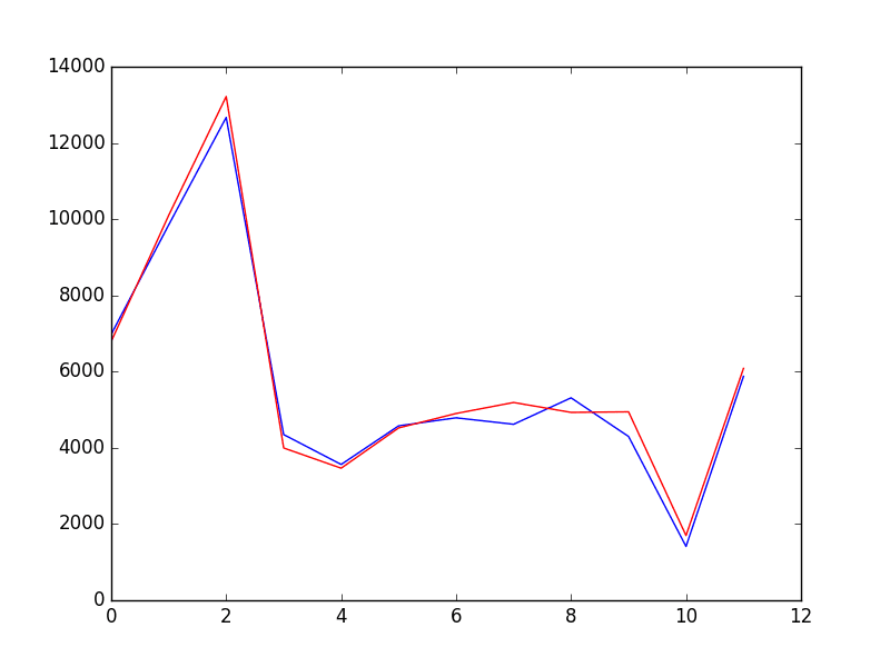
Load the model and use it to forecast the next 12 months. The forecast beyond the first one or two months will quickly start to degrade in skill.
Load the model and use it in a rolling-forecast manner, updating the transform and model for each time step. This is the preferred method as it is how one would use this model in practice as it would achieve the best performance.
As with model evaluation in previous sections, we will make predictions in a rolling-forecast manner. This means that we will step over lead times in the validation dataset and take the observations as an update to the history.
1
2
3
4
5
6
7
8
9
10
11
12
13
14
15
16
17
18
19
20
21
22
23
24
25
26
27
28
29
30
31
32
33
34
35
36
37
38
39
40
41
42
43
44
45
46
47
48
49
50
51
52
53
54
55
56
57
58
59
# load and evaluate the finalized model on the validation dataset
from pandas import read_csv
from matplotlib import pyplot
from statsmodels.tsa.arima.model import ARIMA
from statsmodels.tsa.arima.model import ARIMAResults
Would you recommend this example to a starter. I am totally new to programming and Machine Learning, and I am currently learning Python sytnax and understanding the basic terms around algorithms used.
Hi Benson, this tutorial is an example for a beginner in time series forecasting, but does assume you know your way around Python first (or you can pick it up fast).
Jason, thanks for very detailed instructions on how to construct the model. When I add a few additional periods in the validation set (manually) for a short-term forecast beyond the dataset, the model won’t run until I provide some ‘fake’ targets (expected y). However, when I provide some fake targets, I see that model quickly adjusts to those targets. I tried different levels of y values and I see model predicted accordingly, shouldn’t the predictions be independent of what targets it sees?
Jason, much appreciate your response. What I am trying to convey is that the model should predict same outputs regardless of the observations. For example, when I change y values in my validation set (last 12 months that the model hasn’t seen), my predictions change and the model gives me a very nice RMSE every time. If the model was trained properly, it should have same output for next twelve months regardless of my y values in the validation set. I think you will see this effect very quickly if you also change your y values from validation set. Unless the model is only good for one period forward and needs to continuously adjust based on observed values of last period.
In this specific case we are using walk-forward validation with a model trained for one-step forecasts.
This means as we walk over the validation dataset, observations are moved from validation into training and the model is refit. This is to simulate a new observation being available after a prediction is made for a time step and us being able to update our model in response.
I think what you are talking about is a multi-step forecast, e.g. fitting the model on all of the training data, then forecasting the next n time steps. This is not the experimental setup here, but you are welcome to try it.
I am wondering if it is possible to take into account hierarchy, like the forecast of monthly sales divided in sub-forecasts of french champagne destination markets, using python.
Hi Hugo, yes I am familiar with SARIMA, but I decided to keep the example limited to ARIMA.
Yes, as long as you have the data to train/verify the model. I would consider starting with independent models for each case, using all available data and tease out how to optimize it further after that.
1.
When I’m doing Grid Search ARIMA Hyperparameters with your example, it’s quite slow on my machine, spent about 1 minutes. However the parameter range and data are not large at all. Is it slow specific on my end? I’m concerning the model is too slow to use.
2.
Does ARIMA support multi-step forecast? E.g. What if I keep use predicted value into next forecast, will it overfitting?
Thanks for this awesome hands-on on Time series. However I have a query.
I extracted year and month from date column as my features for model. Then I built a Linear Regression model and a Random Forest model. My final prediction was a weighted average of both these models. I got an rmse of 366 (similar to yours i.e. 361 on validation data).
Can this approach be the alternative for an ARIMA model? What can be the possible drawbacks of this approach?
Jason, I just finished reading “Introduction to Time Series Forecasting in Python” in detail and had two questions:
* Are you planning to come out with a “Intermediate course in Time Series Forecasting in Python” soon?
* You spend the first few chapters discussing how to reframe a time-series problem into a typical Machine Learning problem using Lag features. However, in later chapters, you only use ARIMA models, that obviate the necessity of using explicitly generated lag features. What’s the best way to use explicitly generated timeseries features with other ML algorithms (such as SVM or XGBoost)?
(I tried out a few AR lags with XGB and got decent results using but couldn’t figure out how to incorporate the MA parts).
Would appreciate any insights.
can it be that TimeGrouper() does not work if there are months missing in a year? Also there are no docs available for TimeGrouper(). May you can use pd.Grouper in your future examples?
Hi Jason, I am having the same error. I checked the lines and I have them all. How can python convert ‘yyyy-mm’ to float32?
I dowload the csv from the link of datamarket you gave above.
What am i missing?
Thnanx
Hi Jason , Nice approach for time series forecasting.Thanks for this Article.
Just had a one small doubt,Here we are tuning our ARIMA parameter on test data using RMSE as a measure but generally we tune our parameter on the training(train+validation)data and then we check whether those parameters are well generalized or not by using test data. is it right?
Because my concern is that if we choose our parameter on that particular test data,whether those parameter will generalized to coming new test data or not? I feel that there will be biasness while choosing parameter because we are specifically choosing parameter those giving less RMSE for that test data.Here we are not checking whether our model is working/fitted well for our train data or not?
If i am wrong just correct me.Let me know the logic behind this parameter tuning on the basis of test data?
Hi Jason,
Thank you for this detailed and clear tutorial.
I have a question concerning fiding ARIMA’s parameters. I didn’t understand why we have an imbricated “for” loop and we do consider all the p values and not all the q values.
Thanks for this awesome example! It helped me a lot! However if you don’t mind, I have a question on the prediction loop.
Why did you use history.append(obs) instead of history.append(yhat) when doing the loop for prediction? Sees like you add the observation (real data in test) to history. And yhat = bias + inverse_difference(history, yhat, months_in_year) is based on the history data. but actually we don’t have those observation data when solving practical problem.
I’ve tried to use history.append(yhat) in my model, but the result is worse than using history.append(obs).
Thanks a lot for this work.
I have a point to discuss on concerning the walk forward validation.
I saw that you fill the history part by a value from the test set at each iteration :
…..
# observation
obs = test[i]
history.append(obs)
….
Do we really have to do this or we have to use the new yhat computed for the next predictions?
Indeed when we have to do a future prediction on some range date we don’t have the historical value….
Regards and thanks in advance for your feedback
In this case, we are assuming that the true observations are available after each modeling step and can be used in the formulation of the next prediction, a reasonable assumption, but not required in general.
I was wondering if you could provide the full code to extend the forecast for 1 year ahead. I know you mentioned above that there is a forecast function but when I run:
yhat = model_fit.forecast()[0]
pyplot.plot(y)
pyplot.plot(yhat, color=’green’)
pyplot.plot(predictions, color=’red’)
pyplot.show()
I don’t get any green lines in my code. I’m sure I’m missing a lot of things here, but I don’t know what.
Hi Jason,
I am using this modelling steps to model my problem. When I am passing best parameter which i have got from Grid Search for doing prediction, I am getting Linear Algebra error and sometimes not converging
Due to this I am not able to predict the values.
My second concern is if this is happening for Grid search, how can i automate the script in production environment. Lets say i have to forecast some values for 50000 different sites then what is best way to achieve this goal ?
Thank for your post, it is really helpful for me. It is great!
I have a small question:
In the post, you use 2 data set: dataset.csv and validation.csv
+ In dataset.csv, you split it and use Walk-forward validation -> I totally agree.
+ In validation.csv, you still re-train ARIMA model with walk-forward validation (model_fit = model.fit(trend=’nc’, disp=0) – line 45 in section 7.3) -> I think it is unseen data for testing, so we don’t train model here and only test the model’s performance. Is it correct?
Hi, Jason
First of all, thank you for your wonderful tutorial.
Until now (part 5.4) I just have one doubt: why you plotted a histogram/kde without removing the trend first? If the goal is to see how the distribution shape is similar to Gaussian distribution, doesn’t a trend changes the distribution of data?
Great question, at that point we are early in the analysis. Generally, I’d recommend looking at density plots before and after making the series stationary.
Trend removal generally won’t impact the form of the distribution if we are doing simple linear operations.
Hi Jason,
Thanks for your awesome post. Could you explain how to set the ‘interval’ in the function difference if I only have 1-year data? My dataset is recorded in half an hour, from June 2016 to June 2017. These data number are large in summer and small in winter, i.e. in winter it is between 0-2000, but in summer it is between 5000-14000.
Hi Jason,
Thank you for the post.I want to implement ‘ARIMA’ function instead of using built-in function.
Do you know where I can find the algorithm to implement ‘ARIMA’ function as well understanding that in detail manner?
Thanks for the brief tutorial on Time Series forecasting. I am receiving the error “Given a pandas object and the index does not contain dates” when running the ARIMA model code snippet.
Be sure you copied all of the sample code exactly including indenting, and also be sure you have prepared the data, including removing the footer information from the file.
I have one problem only when i run the rolling forecasts.
I use a different dataset which has temperature values for every minute of the day. I train the model with the first four days and i use the last day as a test dataset. My problem might be because i add the test observation to the history and my arima returns the following error: raise ValueError(“The computed initial AR coefficients are not ”
ValueError: The computed initial AR coefficients are not stationary
You should induce stationarity, choose a different model order, or you can
pass your own start_params.
My x_test dataset contains 1440 rows and i get the error on the 1423 iteration of the loop. Until iteration 1423 the each arima model does not have issues.
I have used a different hyperparameter (Arima 5,1,1) instead, and everything worked. I don’t know if this is the right thing, since 5,0,1 and 5,1,1 had exactly the same RMSE. What is your opinion about that? And please, one final question, my results now are extremely good, with an RMSE less than 0,01. The prediction line in the plot is almost over the the real data line. Does this has to do with the history.append(obs)? I’m not sure i understand correctly why the test observation is added to the history. And what is the difference of doing a prediction in a for loop with a new model for every step compared by using the steps parameter in 1 model?
Sorry for the long questions!
Your tutorials are even better than the books i’m currently reading!
Hey Jason! What i’m trying to say is, maybe the good predictions are because i append the y observation to the history. Why we do this? what is the purpose? If we do not append the y observation then the results are going to be still valid?
Since i do the rolling forecast manner and i introduce a new model for every iteration, why do i need to save a model and do a the first prediction based on that?
Can i simply do the rolling forecast loop to start from 0 instead of 1?
Thank you so much for this amazing tutorial. It really helps me to learn time series forecasting and prepare for my new job. I’m a total beginner in data analysis/science as I’m currently making transition from engineering to data analysis.
But the problem that I’m facing with this tutorial is as I’m running the code, I’m stuck with the final step, “Validate the Model”. I’ve tried to re-copy and re-run the sample code many times but it didn’t seem to work. Here is the error.
/Users/amir/Library/Enthought/Canopy/edm/envs/User/lib/python3.5/site-packages/sklearn/utils/validation.py in _assert_all_finite(X)
56 and not np.isfinite(X).all()):
57 raise ValueError(“Input contains NaN, infinity”
—> 58 ” or a value too large for %r.” % X.dtype)
59
60
ValueError: Input contains NaN, infinity or a value too large for dtype(‘float32’).
Here, what if we append yhat to history, when i am appending yhat to history, my results are really bad, pls help..
Because as per my model, we need to predict the test data by using only the training data, so we cannot use obs to be appended in history, hope you get my point.
Concept wise i understand what is Recursive Multi step forecasting, that’s the same i have used in my earlier reply code, i have appended obs in history, so that means everytime my loop runs, it takes the existing training data + next observation, so that should work and should predict correctly, but my results are really bad..
Or do you mean to say, for this we need to plot the ACF, PACF graph in a a loop to determine the pdq values, and then run the ARIMA function on the pdq values, if that so, pls help us in finding a way to determine pdq values in loop
Thank you for your clear and straightforward post!
I have the same question as Nick above – about the choice of differentiation interval.
In your example you set it to 12 according to the expected cycle of the data.
However, in a more problematic case the data does not seem to imply a clear cycle (ACF and PACF graphs notwithstanding).
In my case, I’ve found out that setting the interval to 12 yielded better results than my default, which was 1. I can understand why choosing a small interval would be generally bad – random noise is too dominant. I have more difficulty understanding how to calibrate the ideal interval value for my data (except brute force, that is. Maybe I shouldn’t calibrate? That could induce overfit. Anyway, I still should find a generally decent value).
And another question. I applied a grid search in order to choose the hyperparameters of my ARIMA model. I fear that bias correction could be counter productive in this case.
Do you have any insights on this subject? Would you perform both (grid search followed by bias correction)? Is the answer data dependent?
I have around more than 1000 of products. I have sales yearly history for last 7 years for each 1000 product. I want to develop a model by which I can predict sales amount for next 3 years.
Could you please help me how do I proceed with evaluate, prediction, validation and interpret the same.
Does anybody know whether statmodels ARIMA uses multi-threading or any other kind of parallelization?
I’m trying to run an analysis based on multiple ARIMA fits on my laptop and thread parallelization increases total runtime rather than decrease it. It seems a single ARIMA fit (part of a single thread) uses several processors at once….
This is an excellent article, and it is super helpful. I had two questions for extension that may have been asked but after reading through the comments, I’m not sure if the same advice applies to me. My question is most similar to Nirmals.
1. I have a dataset with multiple “wines”, each with their own historical sales data
2. This dataset has other variables that aren’t just time related.
For example,
Month 1 Sales Month 2 Sales Month 3 Sales online Reviews,
Wine A
Wine B
Wine C
Wine D
I’m wondering if there’s an extension of this Time Series model that can take into account other variables and other instances of historical data. Let me know if I should clarify.
I haven’t read through it yet, but I think it only takes into account historical data of one instance of multiple variables.
I think it would be interesting to find out how to ensemble the results of my
#1. one instance of historical data (Wine A’s last 3 month sales)
#2. one instance of non-historical variables (Wine A’s online reviews, type, etc.)
To me, # 1’s output is a “variable” to be used in the ML model for #2. If that makes sense, do you think that’s the right way of going about things?
Thank you Jason! for really making ML practitioners like me being awesome in ML.
In this blog you have mentioned that the results suggest that what little autocorrelation is present in the time series has been captured by the model.
What will be the next steps if there is high autocorrelation?
That was a very well informed article! I am trying to forecast on a weekly data. Any tips for improving the model since weekly data is hard to forecast. Also should “months_in_year = 12” used in differencing be changed to “weeks in month=4” to accommodate for weekly frequency?
Hi Jason,
Thank you for an amazing tutorial!
Just one quick question: can you please provide solution for the first scenario (not rolling forward forecast):
– Load the model and use it to forecast the next 12 months. The forecast beyond the first one or two months will quickly start to degrade in skill.
Thank you~
My time series data is non stationary as well and I tried upto 3rd degree of differentiation after which I cant proceed any more as the data is exhausted. It has 3 calculated points and on doing Fuller test for checking stationarity, it errors out “maxlag should be < nobs". What can I do here?
i wonder if we can say that python give good forecasts than other forecast logiciels like Aperia.
To forecast sales we have to base ourselves in historic and baseline but in fact, in industry there are many factors that complexify the calculation of our forecast like the marketing actions, exceptional customer order, … How can we consider these perturbation in our forecasts to ensure good value of accuracy.
First of all, this is a great article, well written and detailed. I have a question regarding on the use of the test set on all of the analysis. What about putting this model in production? You wouldn’t have the ‘test[i]’ (or ‘y[i]’) for each iteration to add to the list ‘history’ to have a truly generalized prediction.
My point is that that instead of adding the values from the test set (‘y[i]’, ‘test[i]’) you’d rather add the predictions being made to the training set in order to do a true random walk.
Thanks again for the resource and all the help putting out this content.
I’m having an issue with the PACF plot for the residuals in part 6.3 Plotting The Residuals. I have followed your code exactly with the ACF plot resulting in a perfect match of the one displayed here tower the PACF is plotting values nearing 8 at around 36 – 38 lags. Any idea what might be causing this?
Hi Jason,
Thanks so much for this tutorial. One thing though. As series.from_csv is depricated, the date format gets lost when opening the dataset, for exemple when trying to generate the seasonal line plots. Are you aware of a workaround that would keep the date format while using read_csv instead of from_csv?
Thanks!
Hi Jason,
I was able to predict and chart looks nice. Just wondering how can we predict for the future, I mean to say if I wanted to see for next month prediction how are we able to do that?
Hi Jason, I deal with daily set data. What is the issue when I try months_in_year = 364?? I mean it’s not throwing best_arima out when I set months_in_year = 364. May I know the reason?
thank you so much for your tutorial. I would like to apply it to a process, forecasting some process variables. The time interval is not monthly based, as in your example, but is much shorter, like some days and the data collection is about every three seconds.
Now I would like to ask some questions.
Do you think that this model could work equally well ?
What should I put in place of ‘months_in_year’ ? For now I put 7, which is the number of different days in my dataset.
Is it normal that with 2000+ points the matrix analysis regarding the seeking of the optimal parameters is taking ages ? (e.g. one triplet after 30 min) If yes, how could I improve the code speed ?
Hi Jeson in running your code I get this error:
raise ValueError(“The computed initial MA coefficients are not ”
ValueError: The computed initial MA coefficients are not invertible
You should induce invertibility, choose a different model order, or you can
pass your own start_params.
How can I solve it? Thank you
Perhaps confirm your statsmodels and other libraries are up to date?
Perhaps confirm that you copied all of the code in order?
Perhaps try an alternative model configuration?
Name Month Qty Unit
Wire Rods Total 2007-JAN 93798 t
Wire Rods Total 2007-FEB 86621 t
Wire Rods Total 2007-MAR 93118 t
My code is :
import pandas as pd
from sklearn.metrics import mean_squared_error
from math import sqrt
# load data
path_to_file = “C:/Users\ARAVIND\Desktop\jupyter notebook\project\datasets.csv”
data = pd.read_csv(path_to_file, encoding=’utf-8′)
# prepare data
X = data.values
X = X.astype(‘float32’)
train_size = int(len(X) * 0.50)
train, test = X[0:train_size], X[train_size:]
# walk-forward validation
history = [x for x in train]
predictions = list()
for i in range(len(test)):
# predict
yhat = history[-1]
predictions.append(yhat)
# observation
obs = test[i]
history.append(obs)
print(‘>Predicted=%.3f, Expected=%3.f’ % (yhat, obs))
# report performance
mse = mean_squared_error(test, predictions)
rmse = sqrt(mse)
print(‘RMSE: %.3f’ % rmse)
when i run this command it shows “Value error: could not convert string to float”… so could anyone tell how to convert string to float according to my dataset.. i want to convert the columns which is “Name, Month and Unit” to float.
However, I get the below error when I am trying to run it on a time series:
ValueError: The computed initial MA coefficients are not invertible
You should induce invertibility, choose a different model order, or you can
pass your own start_params.
This is really a helpful tutorial. Thank you Jason!!
And I have a small question. I got TypeError: a float is required error after i executed this code –
history = [x for x in train]
predictions = list()
for i in range(len(test)):
# predict
yhat = …
predictions.append(yhat)
# observation
obs = test[i]
history.append(obs)
print(‘>Predicted=%.3f, Expected=%3.f’ % (yhat, obs))
What should be the approach when we need to provide long term forecasts ~ 12 months with exogenous variables using a technique like ARIMAX? Should we forecast the covariates and then add it in the model?
Just to be clear, if I add regressors and train the model, I would require future values right? E.g. xreg argument in auto.arima etc. How can I forecast +12 months without utilizing regressors that I have used for training?
That’s a very helpful article. My time series is a daily Point of sale data (eg. how many pepsi bottles get bought everyday in a walmart). There are missing dates when pepsi was not sold at all. What I want to forecast is the bottles of pepsi sold on each day for the next 3/4 days. What might be the best approach/ algorithm?
Hello,
I got exactly same results of the Augmented Dickey-Fuller test, however my PACF plot looks much different, It has a lot of spikes from lag 50 to 80, one even reaching -120.
Any ideas or previous experience why it can look that strange?
Thank you for sharing your knowledge with us.
I have tried with earnest to work through your tutorial. Unfortunately, I am running into errors.
One being this error. This could be the whole bone to my issues. As for the life of me, I could not resolve it using your code alone. I had to tinker with it – see explanation.
series = Series.from_csv(‘dataset.csv’)
AttributeError: type object ‘Series’ has no attribute ‘from_csv’
Which I resloved by implementing
panda import pd
series = pd.read_csv(‘dataset.csv’)
series.iloc[0]
Once I got over that hurdle – I then ran into this hurdle.
dataset = dataset.astype(‘float32’)
ValueError: could not convert string to float: ‘1964-01’
More than like its something I am doing wrong.
Would it be at all possible to have access to the full code? My attempts in copying and pasting obviously are not helping me.
I think I have possibly left some intrinsic part of the code out. Or I have totally confused myself.
Hi jason,
I was wondering if you have used fbprophet for sales prediction. We were fetching data directly from postgresql and we seem to be running into an error
Out of bounds nanosecond timestamp: 1-08-11 00:00:00
This seems to be something related with pandas version compatibility.
Could you please look into it and try to find the problem behind it?
I’m running the
series=read_csv(r’D:\industrial engineering\Thesis\monthly_champagne_sales.csv’,header=0,index_col=0)
code and what I’m getting is a data frame, not a Series what should I do?
dear sir
I am running following code in a rolling window framework however, i am not able to see results that come from the analysis. It displays only one value. Can you please let me know what and where i need to fix so that i can get those results:
##Entropy
from entropy import *
import numpy as np
np.random.seed(1234567)
x = np.random.rand(3000)
n = len(x)
result = list()
block = 250
for a in range(1, n-block+1):
DATA = x[a:a+249]
results = perm_entropy(DATA, order=3, normalize=True)
result.append(results)
return Series(result)
I would like to ask you about TS with repeating dates. For example, I have a dataset with different type of deals and the deals have different time periods depending on their agreement. Which means, when a stationary graph is plotted there can be more than one observation (revenue in my case) on each date. For example, 2/11/2018 could have multiple revenue from different deals. Therefore, the graph sketch is very confusing in the sense that there are many/few repetition on the same date. My idea is to sum the revenues up by date but would that affect the accuracy of the model as the prediction should be by deals? Your thoughts and reply would be highly appreciated. Regards
Hi Jason,
Thank you so much for publishing this article. Most articles that I have found simply tell a user what to enter into each field for their specific example, without really getting in what a parameter means or how it is used. As a result, I haven’t been able to get my arms around what to enter for my situation. Your article does a nice job of explaining how you came up with your parameters. I do have a question, though. What should I do differently for a small dataset? I only have about 30 months of data for what I am trying to predict. For the purposes of going through this tutorial, I faked some data. In doing so, it is providing me with negative sales predictions. Is that enough data to provide an accurate forecast?
One additional note, in 7.3 you have the code:
series = read_csv(‘dataset.csv’, header=None, index_col=0, parse_dates=True, squeeze=True)
X = dataset.values.astype(‘float32’)
I believe that it should be:
series = read_csv(‘dataset.csv’, header=None, index_col=0, parse_dates=True, squeeze=True)
X = series.values.astype(‘float32’)
Absolutely great exercise. Loved it…
Just one quick question:
How do I generate a forecast for next 12 intervals and generate a plot with training, test and predicted together
After read your great post (as usual) I have a couple of questions.
First is about residuals. You have calculated manually and then use a dataframe to work with them later. But, I have read arima.fit results have a member called residuals. I’ve been working in an different serie using those residuals, before read your article. Then I did that manually as you did. BUT both are different, and not such slightly different.. Should both be similar? Because I think they should and as many times I’m looking for an bug in my code
Second is about differences. when you make a diff to the serie you lose some elements, depending on lags. Well you can preserve the original data, so it is possible to integrate.It is academically perfect. But what to do when you have just only the final model? I mean when you recover new data and want to make a new prediction, the model will bring you predictions over transformed data you need to reescale. If you have used standardization you can get values to detransform but How you can integrate ? there information lost…
Couldn’t understand why bias is added to the predicted value.
“yhat = bias + inverse_difference(history, yhat, months_in_year)” .
Also , is there a possibility of not getting the exact values as shown in this post , when I run the code ? Any reasons why ?
Hey Jason I like your example I just have a question about putting in my own data. So my data has a count of visits for everyday of the year for 2019 and so far in 2020. I am wondering if since this does everyday instead of months months_in_year = 12 do I change months_in_year = 12 to days_in_year = 365?
Hey Jason ,am impressed by your commitment, and would you mind to show me about features/attributes of sales dataset to forecast Future sales of a supper market using deep learning/LSTM algorithm
Thanks for your tutorials. Very helpful indeed. After differencing, I made the series stationary and now for the ARIMA, I wanna plot the ACF and the PACF. These are my codes –
1) Code for differencing to make the data stationary
from pandas import read_csv
from statsmodels.tsa.stattools import adfuller
from numpy import diff
X = diff(X)
result = adfuller(X)
print(‘ADF Statistic: %f’ % result[0])
print(‘p-value: %f’ % result[1])
for key, value in result[4].items():
print(‘\t%s: %.3f’ % (key, value))
2) Code to plot the ACF and the PACF
from pandas import read_csv
from statsmodels.graphics.tsaplots import plot_acf
from statsmodels.graphics.tsaplots import plot_pacf
from matplotlib import pyplot
series = read_csv(‘X.csv’, header=None, index_col=0, parse_dates=True, squeeze=True)
pyplot.figure()
pyplot.subplot(211)
plot_acf(series, ax=pyplot.gca())
pyplot.subplot(212)
plot_pacf(series, ax=pyplot.gca())
pyplot.show()
After running the second code, I am getting an error which is –
FileNotFoundError Traceback (most recent call last)
in
3 from statsmodels.graphics.tsaplots import plot_pacf
4 from matplotlib import pyplot
—-> 5 series = read_csv(‘X.csv’, header=None, index_col=0, parse_dates=True, squeeze=True)
6 pyplot.figure()
7 pyplot.subplot(211)
Hi, I’m new to python and trying to learn from your blog.
Would you mind to explain your codes for the following? I don’t understand what is obs. Is yhat the predicted result?
obs = test[i]
history.append(obs)
print(‘>Predicted=%.3f, Expected=%3.f’ % (yhat, obs))
Thank you so much for this very educational step by step blog!!
yhat is a prediction made by the predictive model.
In the code – we are storing the real observation in history – we are pretending the real observation just became available after we made a prediction so we add it to training data on the next iteration.
I have a query. Can I forecast if I have a dataset of 10 years only. If yes, in that case how will I divide my dataset into Training and Testing dataset ?
Quick question, I am not getting the same results when running the manual ARIMA model. Your results of 956.942 vs. my 961. Everythign else matched up until that point but I was having issues with autocorrelation plots only showing 21 observations vs 81 as well. Any help is greatly appreciated.
# evaluate manually configured ARIMA model
from pandas import read_csv
from sklearn.metrics import mean_squared_error
from statsmodels.tsa.arima.model import ARIMA
from math import sqrt
# create a differenced series
def difference(dataset, interval=1):
diff = list()
for i in range(interval, len(dataset)):
value = dataset[i] – dataset[i – interval]
diff.append(value)
return diff
Hi Jason, thanks a lot god this. I would like to know the reason for using seasonally differenced data for the ARIMA model. I have followed the previous example (robbery dataset) and the differences wasn’t used with ARIMA model.
Nice tutorial. By the way, What if I have unequal time length in my data. Say I have sales data for 8 month from 2019, 6 months from 2020. and 10 months from 2021. How can I build model using unequal number of months? Thank you so much for your time!
This means that the interval between the observations is not consistent, but may vary.
You can learn more about contiguous vs discontiguous time series datasets in this post:
Taxonomy of Time Series Forecasting Problems
There are many ways to handle data in this form and you must discover the approach that works well or best for your specific dataset and chosen model.
The most common approach is to frame the discontiguous time series as contiguous and the observations for the newly observation times as missing (e.g. a contiguous time series with missing values).
Some ideas you may want to explore include:
Ignore the discontiguous nature of the problem and model the data as-is.
Resample the data (e.g. upsample) to have a consistent interval between observations.
Impute the observations to form a consistent interval.
Pad the observations for form a consistent interval and use a Masking layer to ignore the padded values.
Hi James, Thanks for your reply. Problem here that store opening depends on the weather condition of a year. It doesn’t operate same time of each year. It varies! It was open only r 8 month from 2019, 6 months from 2020. and 10 months from 2021. How can we treat this as missing value problem? Any workout tutorial would be great! I appreciate your time!Thanks!
Hello, I would like to ask a qion, because my data set is to record the plant harvest data, and the month is relatively fixed, so each year only two months of data, for example, the 2021 has 48 days of data, there are 50 days in 2022, so based on that, should I fill in all the dates that don’t have data with zeros? Does this also mean a seasonal figure? If I make a prediction using SARIMAX, what should I do with my cycle?


Thank You Jason.
Would you recommend this example to a starter. I am totally new to programming and Machine Learning, and I am currently learning Python sytnax and understanding the basic terms around algorithms used.
Regards,
Benson
Hi Benson, this tutorial is an example for a beginner in time series forecasting, but does assume you know your way around Python first (or you can pick it up fast).
A surely steep learning curve taking you out of your comfort zone, but that’s the way to learn. ?
For sure. Dive in!
helo jason will i be able to contact you and discuss, need explaination..
You can use the contact page to contact me any time via email:
https://machinelearningmastery.com/contact/
Jason, thanks for very detailed instructions on how to construct the model. When I add a few additional periods in the validation set (manually) for a short-term forecast beyond the dataset, the model won’t run until I provide some ‘fake’ targets (expected y). However, when I provide some fake targets, I see that model quickly adjusts to those targets. I tried different levels of y values and I see model predicted accordingly, shouldn’t the predictions be independent of what targets it sees?
You should not need fake targets Viral.
You can forecast a new out of sample data point by training the model on all of the available data and predicting one-step. E.g.:
Jason, much appreciate your response. What I am trying to convey is that the model should predict same outputs regardless of the observations. For example, when I change y values in my validation set (last 12 months that the model hasn’t seen), my predictions change and the model gives me a very nice RMSE every time. If the model was trained properly, it should have same output for next twelve months regardless of my y values in the validation set. I think you will see this effect very quickly if you also change your y values from validation set. Unless the model is only good for one period forward and needs to continuously adjust based on observed values of last period.
In this specific case we are using walk-forward validation with a model trained for one-step forecasts.
This means as we walk over the validation dataset, observations are moved from validation into training and the model is refit. This is to simulate a new observation being available after a prediction is made for a time step and us being able to update our model in response.
I think what you are talking about is a multi-step forecast, e.g. fitting the model on all of the training data, then forecasting the next n time steps. This is not the experimental setup here, but you are welcome to try it.
Hello Jason,
If you don’t mind me asking, where exactly should the line below fit?:
yhat = model_fit.forecast()[0]
Hi Benson,
Fit the ARIMA model on all of your data.
After that, make a forecast for the next time step by calling the forecast() function.
Time to upgrade to matplotlib 2.0, the colors are nicer 🙂
I agree Juanlu! I have recently upgraded myself.
Dear Jason,
Thanks for the post. Clear, concise and working.
Have you considered to forecast the TS using a SARIMA model instead of substracting the seasonality and adding it latter? As a matter of fact, statsmodel has it integrated in its dev version. (http://www.statsmodels.org/dev/generated/statsmodels.tsa.statespace.sarimax.SARIMAX.html)
I am wondering if it is possible to take into account hierarchy, like the forecast of monthly sales divided in sub-forecasts of french champagne destination markets, using python.
Thanks and keep posting!
Hi Hugo, yes I am familiar with SARIMA, but I decided to keep the example limited to ARIMA.
Yes, as long as you have the data to train/verify the model. I would consider starting with independent models for each case, using all available data and tease out how to optimize it further after that.
Thanks for the wonderful post Jason,
Two quick question:
1.
When I’m doing Grid Search ARIMA Hyperparameters with your example, it’s quite slow on my machine, spent about 1 minutes. However the parameter range and data are not large at all. Is it slow specific on my end? I’m concerning the model is too slow to use.
2.
Does ARIMA support multi-step forecast? E.g. What if I keep use predicted value into next forecast, will it overfitting?
Thanks!
Your timing sounds fine. If it is too slow for you, consider working with a sub-sample of your data.
You can do multi-step forecasting directly (forecast() function) or by using the ARIMA model recursively:
https://machinelearningmastery.com/multi-step-time-series-forecasting/
Thanks in advice.
Hello Jason
Thanks for this awesome hands-on on Time series. However I have a query.
I extracted year and month from date column as my features for model. Then I built a Linear Regression model and a Random Forest model. My final prediction was a weighted average of both these models. I got an rmse of 366 (similar to yours i.e. 361 on validation data).
Can this approach be the alternative for an ARIMA model? What can be the possible drawbacks of this approach?
Appreciate your comments
Thanks
Nice work. ARIMA may be a simpler model if model complexity is important on a project.
Hi just a silly note have you consider using itertools for your evaluate_models() function?
https://pastebin.com/w0apb6Tg
in python nested loops are not so readable.
Thanks for the suggestion.
Jason, I just finished reading “Introduction to Time Series Forecasting in Python” in detail and had two questions:
* Are you planning to come out with a “Intermediate course in Time Series Forecasting in Python” soon?
* You spend the first few chapters discussing how to reframe a time-series problem into a typical Machine Learning problem using Lag features. However, in later chapters, you only use ARIMA models, that obviate the necessity of using explicitly generated lag features. What’s the best way to use explicitly generated timeseries features with other ML algorithms (such as SVM or XGBoost)?
(I tried out a few AR lags with XGB and got decent results using but couldn’t figure out how to incorporate the MA parts).
Would appreciate any insights.
I may have a more advanced TS book in the future.
Great question. You would have to calculate the MA features manually.
Hi Jason,
can it be that TimeGrouper() does not work if there are months missing in a year? Also there are no docs available for TimeGrouper(). May you can use pd.Grouper in your future examples?
Regards
I think it does work with missing data, allowing you to resample.
TimeGrouper does not have docs, but Grouper does and is a good start:
https://pandas.pydata.org/pandas-docs/stable/generated/pandas.Grouper.html
Hi,
Thanks for this great link on time series.
I am not able to acces the dataset stored at:- https://datamarket.com/data/set/22r5/perrin-freres-monthly-champagne-sales-millions-64-72#!ds=22r5&display=line
Regards,
Sambit
I’m sorry to hear that, here is the full dataset:
hi,
i am having the following error:
X = X.astype(‘float32’)
ValueError: could not convert string to float: ‘1972-09’
can you please help me
ty
Looks like you may have missed some lines of code. Confirm you have them all.
Hi Jason, I am having the same error. I checked the lines and I have them all. How can python convert ‘yyyy-mm’ to float32?
I dowload the csv from the link of datamarket you gave above.
What am i missing?
Thnanx
I have some suggestions here:
https://machinelearningmastery.com/faq/single-faq/why-does-the-code-in-the-tutorial-not-work-for-me
Hi Jason , Nice approach for time series forecasting.Thanks for this Article.
Just had a one small doubt,Here we are tuning our ARIMA parameter on test data using RMSE as a measure but generally we tune our parameter on the training(train+validation)data and then we check whether those parameters are well generalized or not by using test data. is it right?
Because my concern is that if we choose our parameter on that particular test data,whether those parameter will generalized to coming new test data or not? I feel that there will be biasness while choosing parameter because we are specifically choosing parameter those giving less RMSE for that test data.Here we are not checking whether our model is working/fitted well for our train data or not?
If i am wrong just correct me.Let me know the logic behind this parameter tuning on the basis of test data?
Yes, that is a less biased way to prepare a model.
More here:
https://machinelearningmastery.com/difference-test-validation-datasets/
Thank you so much Jason.
You’re welcome sandip.
Hi Jason,
Thank you for this detailed and clear tutorial.
I have a question concerning fiding ARIMA’s parameters. I didn’t understand why we have an imbricated “for” loop and we do consider all the p values and not all the q values.
Please ask if the question is not that clear.
Thank you in advance.
Please review the example again, we grid search p, d and q values.
Hi Jason,
Thanks for this awesome example! It helped me a lot! However if you don’t mind, I have a question on the prediction loop.
Why did you use history.append(obs) instead of history.append(yhat) when doing the loop for prediction? Sees like you add the observation (real data in test) to history. And yhat = bias + inverse_difference(history, yhat, months_in_year) is based on the history data. but actually we don’t have those observation data when solving practical problem.
I’ve tried to use history.append(yhat) in my model, but the result is worse than using history.append(obs).
Appreciate your comments
Thanks,
Ella
Good question, because in this scenario, we are assuming that each new real observation is available after we make a prediction.
Pretend we are running this loop one iteration per day, and we get yesterdays observation this morning so we can accurately predict tomorrow.
Thank you so much for your explanation!!
You’re welcome.
Hello,
Thanks a lot for this work.
I have a point to discuss on concerning the walk forward validation.
I saw that you fill the history part by a value from the test set at each iteration :
…..
# observation
obs = test[i]
history.append(obs)
….
Do we really have to do this or we have to use the new yhat computed for the next predictions?
Indeed when we have to do a future prediction on some range date we don’t have the historical value….
Regards and thanks in advance for your feedback
Simo
It depends on your model and project goals.
In this case, we are assuming that the true observations are available after each modeling step and can be used in the formulation of the next prediction, a reasonable assumption, but not required in general.
If you use outputs as inputs (e.g. recursive multi-step forecasting), error will compound and things will go more crazy, sooner (e.g. model skill will drop). See this post:
https://machinelearningmastery.com/multi-step-time-series-forecasting/
Sorry, I just read the Ella question…So for long range future prediction we have ti use the yhat…
Thanks
You can if you choose.
Hi,
I am getting NAN after these steps:
from pandas import Series
series = Series.from_csv(‘champagne.csv’, header=0)
print(len(series))
split_point = len(series) – 12
print(split_point)
dataset, validation = series[0:split_point], series[split_point:]
print(dataset)
print(‘Dataset %d, Validation %d’ % (len(dataset), len(validation)))
dataset.to_csv(‘dataset.csv’)
validation.to_csv(‘validation.csv’)
I’m sorry to hear that.
Ensure that you have copied all of the code and that you have removed the footer from the data file. Also confirm that your environment is up to date.
Hi Jason,
This is extremely useful. Thank you very much!
I was wondering if you could provide the full code to extend the forecast for 1 year ahead. I know you mentioned above that there is a forecast function but when I run:
yhat = model_fit.forecast()[0]
pyplot.plot(y)
pyplot.plot(yhat, color=’green’)
pyplot.plot(predictions, color=’red’)
pyplot.show()
I don’t get any green lines in my code. I’m sure I’m missing a lot of things here, but I don’t know what.
Thank you again, much appreciated!
This post will help you with making longer-term forecasts:
https://machinelearningmastery.com/make-sample-forecasts-arima-python/
Hi Jason,
I am using this modelling steps to model my problem. When I am passing best parameter which i have got from Grid Search for doing prediction, I am getting Linear Algebra error and sometimes not converging
Due to this I am not able to predict the values.
My second concern is if this is happening for Grid search, how can i automate the script in production environment. Lets say i have to forecast some values for 50000 different sites then what is best way to achieve this goal ?
Sorry to hear that, perhaps you have not set all of the parameters the same as you used in the grid search?
I have some notes about models in production here that may help:
https://machinelearningmastery.com/deploy-machine-learning-model-to-production/
Hi Jason,
Thank for your post, it is really helpful for me. It is great!
I have a small question:
In the post, you use 2 data set: dataset.csv and validation.csv
+ In dataset.csv, you split it and use Walk-forward validation -> I totally agree.
+ In validation.csv, you still re-train ARIMA model with walk-forward validation (model_fit = model.fit(trend=’nc’, disp=0) – line 45 in section 7.3) -> I think it is unseen data for testing, so we don’t train model here and only test the model’s performance. Is it correct?
In the case of walk forward validation, we are assuming that the real observations are available after the time of prediction.
You can make different assumptions when evaluating your model.
Hi, Jason
First of all, thank you for your wonderful tutorial.
Until now (part 5.4) I just have one doubt: why you plotted a histogram/kde without removing the trend first? If the goal is to see how the distribution shape is similar to Gaussian distribution, doesn’t a trend changes the distribution of data?
Thanks
Navid
Great question, at that point we are early in the analysis. Generally, I’d recommend looking at density plots before and after making the series stationary.
Trend removal generally won’t impact the form of the distribution if we are doing simple linear operations.
Hi Jason,
Thanks for your awesome post. Could you explain how to set the ‘interval’ in the function difference if I only have 1-year data? My dataset is recorded in half an hour, from June 2016 to June 2017. These data number are large in summer and small in winter, i.e. in winter it is between 0-2000, but in summer it is between 5000-14000.
Hi Jason,
Thank you for the post.I want to implement ‘ARIMA’ function instead of using built-in function.
Do you know where I can find the algorithm to implement ‘ARIMA’ function as well understanding that in detail manner?
A good textbook on the math is this one: http://amzn.to/2zvfIcB
Hi Jason,
Thanks for the brief tutorial on Time Series forecasting. I am receiving the error “Given a pandas object and the index does not contain dates” when running the ARIMA model code snippet.
Be sure you copied all of the sample code exactly including indenting, and also be sure you have prepared the data, including removing the footer information from the file.
Dear Jason,
Thanks for your amazing tut!
I have one problem only when i run the rolling forecasts.
I use a different dataset which has temperature values for every minute of the day. I train the model with the first four days and i use the last day as a test dataset. My problem might be because i add the test observation to the history and my arima returns the following error: raise ValueError(“The computed initial AR coefficients are not ”
ValueError: The computed initial AR coefficients are not stationary
You should induce stationarity, choose a different model order, or you can
pass your own start_params.
for i in range(0, len(x_test)):
# difference data
diff = difference(history, minutes)
# predict
model = importer.ARIMA(diff, order=(5, 0, 1))
model_fit = model.fit(trend=’nc’, disp=0)
yhat = model_fit.forecast()[0]
yhat = inverse_difference(history, yhat, minutes)
predictions.append(yhat)
# observation
obs = x_test[i]
history.append(obs)
print(‘Predicted=%.6f, Expected=%.6f’ % (yhat, obs))
My x_test dataset contains 1440 rows and i get the error on the 1423 iteration of the loop. Until iteration 1423 the each arima model does not have issues.
Your help is precious to me.
Thanks again!
Kindest Regards,
Makis
Have you confirmed that your data set is stationary? Perhaps there is still some trend or seasonal structure?
I have many posts on detrending and seasonal adjustment that may help.
Dear Jason,
Thanks for your response!
I have used a different hyperparameter (Arima 5,1,1) instead, and everything worked. I don’t know if this is the right thing, since 5,0,1 and 5,1,1 had exactly the same RMSE. What is your opinion about that? And please, one final question, my results now are extremely good, with an RMSE less than 0,01. The prediction line in the plot is almost over the the real data line. Does this has to do with the history.append(obs)? I’m not sure i understand correctly why the test observation is added to the history. And what is the difference of doing a prediction in a for loop with a new model for every step compared by using the steps parameter in 1 model?
Sorry for the long questions!
Your tutorials are even better than the books i’m currently reading!
Cheers from Greece.
Well done. I’d recommend using the model that is skillful and stable.
Hey Jason! What i’m trying to say is, maybe the good predictions are because i append the y observation to the history. Why we do this? what is the purpose? If we do not append the y observation then the results are going to be still valid?
In the test setup we are assuming that real observations are made after each prediction that we can in turn use to make the next prediction.
Your specific framing of the problem may differ and I would encourage you to design a test harness to capture that.
Hey Jason, for once more thanks for your feedback!
I will follow your suggestion right now 🙂
Thanks for everything
Kind Regards,
Makis
Hey Jason, one last question.
Since i do the rolling forecast manner and i introduce a new model for every iteration, why do i need to save a model and do a the first prediction based on that?
Can i simply do the rolling forecast loop to start from 0 instead of 1?
Sure.
Hi Jason,
Thank you so much for this amazing tutorial. It really helps me to learn time series forecasting and prepare for my new job. I’m a total beginner in data analysis/science as I’m currently making transition from engineering to data analysis.
But the problem that I’m facing with this tutorial is as I’m running the code, I’m stuck with the final step, “Validate the Model”. I’ve tried to re-copy and re-run the sample code many times but it didn’t seem to work. Here is the error.
>Predicted=10101.763, Expected=9851
>Predicted=13219.067, Expected=12670
>Predicted=3996.535, Expected=4348
>Predicted=3465.934, Expected=3564
>Predicted=4522.683, Expected=4577
>Predicted=4901.336, Expected=4788
>Predicted=5190.094, Expected=4618
>Predicted=4930.190, Expected=5312
>Predicted=4944.785, Expected=4298
>Predicted=1699.409, Expected=1413
>Predicted=6085.324, Expected=5877
>Predicted=7135.720, Expected=nan
ValueError Traceback (most recent call last)
in ()
56
57 # Report performance
—> 58 mse = mean_squared_error(y, predictions)
59 rmse = sqrt(mse)
60 print(‘RMSE: %.3f’ % rmse)
/Users/amir/Library/Enthought/Canopy/edm/envs/User/lib/python3.5/site-packages/sklearn/metrics/regression.py in mean_squared_error(y_true, y_pred, sample_weight, multioutput)
229 “””
230 y_type, y_true, y_pred, multioutput = _check_reg_targets(
–> 231 y_true, y_pred, multioutput)
232 output_errors = np.average((y_true – y_pred) ** 2, axis=0,
233 weights=sample_weight)
/Users/amir/Library/Enthought/Canopy/edm/envs/User/lib/python3.5/site-packages/sklearn/metrics/regression.py in _check_reg_targets(y_true, y_pred, multioutput)
73 “””
74 check_consistent_length(y_true, y_pred)
—> 75 y_true = check_array(y_true, ensure_2d=False)
76 y_pred = check_array(y_pred, ensure_2d=False)
77
/Users/amir/Library/Enthought/Canopy/edm/envs/User/lib/python3.5/site-packages/sklearn/utils/validation.py in check_array(array, accept_sparse, dtype, order, copy, force_all_finite, ensure_2d, allow_nd, ensure_min_samples, ensure_min_features, warn_on_dtype, estimator)
405 % (array.ndim, estimator_name))
406 if force_all_finite:
–> 407 _assert_all_finite(array)
408
409 shape_repr = _shape_repr(array.shape)
/Users/amir/Library/Enthought/Canopy/edm/envs/User/lib/python3.5/site-packages/sklearn/utils/validation.py in _assert_all_finite(X)
56 and not np.isfinite(X).all()):
57 raise ValueError(“Input contains NaN, infinity”
—> 58 ” or a value too large for %r.” % X.dtype)
59
60
ValueError: Input contains NaN, infinity or a value too large for dtype(‘float32’).
Could you please help me with this?
Thank you so much
Amir
I’m not sure of the cause of your fault, sorry.
Ensure your libraries are up to date and that you have copied all of the code exactly?
The csv file contains some jargon text which should be deleted before reading the file as list.
Hi Jason,
In the prediction area, where you have added the observation to history and then running the loop to find the ARIMA results.
i.e.
model = ARIMA(history, order=(4,1,2))
model_fit = model.fit(disp=0)
output = model_fit.forecast()
yhat = output[0]
predictions.append(yhat)
obs = test[t]
history.append(obs)
Here, what if we append yhat to history, when i am appending yhat to history, my results are really bad, pls help..
Because as per my model, we need to predict the test data by using only the training data, so we cannot use obs to be appended in history, hope you get my point.
Yes, that would be called a recursive multi-step forecast. It is challenging. You can learn a little more about it here:
https://machinelearningmastery.com/multi-step-time-series-forecasting/
Concept wise i understand what is Recursive Multi step forecasting, that’s the same i have used in my earlier reply code, i have appended obs in history, so that means everytime my loop runs, it takes the existing training data + next observation, so that should work and should predict correctly, but my results are really bad..
Or do you mean to say, for this we need to plot the ACF, PACF graph in a a loop to determine the pdq values, and then run the ARIMA function on the pdq values, if that so, pls help us in finding a way to determine pdq values in loop
Generally using forecasts in a recursive model is challenging, you may need to get creative with your model/models.
Hello Jason,
Thank you for your clear and straightforward post!
I have the same question as Nick above – about the choice of differentiation interval.
In your example you set it to 12 according to the expected cycle of the data.
However, in a more problematic case the data does not seem to imply a clear cycle (ACF and PACF graphs notwithstanding).
In my case, I’ve found out that setting the interval to 12 yielded better results than my default, which was 1. I can understand why choosing a small interval would be generally bad – random noise is too dominant. I have more difficulty understanding how to calibrate the ideal interval value for my data (except brute force, that is. Maybe I shouldn’t calibrate? That could induce overfit. Anyway, I still should find a generally decent value).
If the amount of data is relatively small, consider using a grid search across difference values to see what works.
And another question. I applied a grid search in order to choose the hyperparameters of my ARIMA model. I fear that bias correction could be counter productive in this case.
Do you have any insights on this subject? Would you perform both (grid search followed by bias correction)? Is the answer data dependent?
I would only perform bias correction if it lifted model skill (e.g. if the model was biased).
Hi Jason,
I have around more than 1000 of products. I have sales yearly history for last 7 years for each 1000 product. I want to develop a model by which I can predict sales amount for next 3 years.
Could you please help me how do I proceed with evaluate, prediction, validation and interpret the same.
Thanking in advance.
Perhaps start here:
https://machinelearningmastery.com/start-here/#timeseries
(Noob’s parallelization question, probably)
Does anybody know whether statmodels ARIMA uses multi-threading or any other kind of parallelization?
I’m trying to run an analysis based on multiple ARIMA fits on my laptop and thread parallelization increases total runtime rather than decrease it. It seems a single ARIMA fit (part of a single thread) uses several processors at once….
Thanks,
Udi
I think it is single threaded.
Hi Jason,
This is an excellent article, and it is super helpful. I had two questions for extension that may have been asked but after reading through the comments, I’m not sure if the same advice applies to me. My question is most similar to Nirmals.
1. I have a dataset with multiple “wines”, each with their own historical sales data
2. This dataset has other variables that aren’t just time related.
For example,
Month 1 Sales Month 2 Sales Month 3 Sales online Reviews,
Wine A
Wine B
Wine C
Wine D
I’m wondering if there’s an extension of this Time Series model that can take into account other variables and other instances of historical data. Let me know if I should clarify.
Thank you for taking the time to clarify.
Yes, perhaps you could model each series separately, or groups of series or all together, or all 3 approaches and ensemble the results.
Also, I’d recommend moving on to other models, such as ML or even MLP models.
I hope to cover this topic in more detail soon.
Thanks for the quick reply.
I’ll try out your first method.
But do you have any good ML/MLP models/tutorials to start with? It’s okay if you don’t! I noticed you have a nice article on multivariate time series here:
https://machinelearningmastery.com/multivariate-time-series-forecasting-lstms-keras/
I haven’t read through it yet, but I think it only takes into account historical data of one instance of multiple variables.
I think it would be interesting to find out how to ensemble the results of my
#1. one instance of historical data (Wine A’s last 3 month sales)
#2. one instance of non-historical variables (Wine A’s online reviews, type, etc.)
To me, # 1’s output is a “variable” to be used in the ML model for #2. If that makes sense, do you think that’s the right way of going about things?
Thanks for being so responsive!
I hope to cover this topic in more detail soon – maybe write a book on the topic working one dataset from many different directions.
Thank you Jason! for really making ML practitioners like me being awesome in ML.
In this blog you have mentioned that the results suggest that what little autocorrelation is present in the time series has been captured by the model.
What will be the next steps if there is high autocorrelation?
Thanks in advance.
Great question!
Some ideas:
– Perhaps try alternate models.
– Perhaps improve the data preparation.
– Perhaps try downstream models to further correct the forecast.
Hey Jason,
That was a very well informed article! I am trying to forecast on a weekly data. Any tips for improving the model since weekly data is hard to forecast. Also should “months_in_year = 12” used in differencing be changed to “weeks in month=4” to accommodate for weekly frequency?
Thanks
My best tips are to try lots of data preparation techniques and tune the ARIMA using a grid search.
Hi Jason,
Thank you for an amazing tutorial!
Just one quick question: can you please provide solution for the first scenario (not rolling forward forecast):
– Load the model and use it to forecast the next 12 months. The forecast beyond the first one or two months will quickly start to degrade in skill.
Thank you~
Yes, this will help:
https://machinelearningmastery.com/make-sample-forecasts-arima-python/
Hi Jason
My time series data is non stationary as well and I tried upto 3rd degree of differentiation after which I cant proceed any more as the data is exhausted. It has 3 calculated points and on doing Fuller test for checking stationarity, it errors out “maxlag should be < nobs". What can I do here?
Sounds like you might be running out of data in your series. Perhaps you need more observations?
Hello, thank you.
i wonder if we can say that python give good forecasts than other forecast logiciels like Aperia.
To forecast sales we have to base ourselves in historic and baseline but in fact, in industry there are many factors that complexify the calculation of our forecast like the marketing actions, exceptional customer order, … How can we consider these perturbation in our forecasts to ensure good value of accuracy.
Thank you for answering.
What is Aperia?
Additional elements could be used as exogenous variables in the model.
Jason,
The dataset I have requires to double difference in order to make it stationary, so i used:
diff1 = difference(history, 12)
diff2 = difference(diff1, 12),
it worked and made it stationary with ADF test, however, how do I reverse it back please?
Thank you
Add the values back. It requires that you keep the original and the first diffed data.
Thanks, so would the function look like this?
yhat = inverse_difference(diff1, yhat, interval)
yhat = inverse_difference(history, yhat, interval) ?
Thank you!
Correct.
First of all, this is a great article, well written and detailed. I have a question regarding on the use of the test set on all of the analysis. What about putting this model in production? You wouldn’t have the ‘test[i]’ (or ‘y[i]’) for each iteration to add to the list ‘history’ to have a truly generalized prediction.
My point is that that instead of adding the values from the test set (‘y[i]’, ‘test[i]’) you’d rather add the predictions being made to the training set in order to do a true random walk.
Thanks again for the resource and all the help putting out this content.
A final model will be created by training it on all available data and then using it to make predictions in the future.
You can learn more about final models here:
https://machinelearningmastery.com/train-final-machine-learning-model/
You can learn more about making out of sample predictions here:
https://machinelearningmastery.com/make-sample-forecasts-arima-python/
I keep getting errors
—————————————————————————
TypeError Traceback (most recent call last)
in ()
9 obs = test[i]
10 history.append(obs)
—> 11 print(‘>Predicted=%.3f, Expected=%3.f’ % (yhat, obs))
TypeError: must be real number, not ellipsis
IE: # predict
yhat = …
those 3 dots (ellipsis) are throwing errors.
The code has … throughout. Any idea how to fix this error?
The code with “…” is just example code, it is not for execution. Skip it.
Perhaps a more careful read of the tutorial is in order James?
I’m having an issue with the PACF plot for the residuals in part 6.3 Plotting The Residuals. I have followed your code exactly with the ACF plot resulting in a perfect match of the one displayed here tower the PACF is plotting values nearing 8 at around 36 – 38 lags. Any idea what might be causing this?
Hi Jason,
Thanks so much for this tutorial. One thing though. As series.from_csv is depricated, the date format gets lost when opening the dataset, for exemple when trying to generate the seasonal line plots. Are you aware of a workaround that would keep the date format while using read_csv instead of from_csv?
Thanks!
Yes you can use pandas.read_csv() with the same arguments.
How can I improve the readability of Seasonal Per Year Line Plots (especially when it comes to axes) ? I would be grateful for your help.
Perhaps create one plot per figure?
I’d rather have a comparison between all the subplots.
Perhaps plot them all on the same figure?
Perhaps calculate the different and plot that?
Hi Jason,
I was able to predict and chart looks nice. Just wondering how can we predict for the future, I mean to say if I wanted to see for next month prediction how are we able to do that?
Thanks,
Chintan
I show how here:
https://machinelearningmastery.com/make-sample-forecasts-arima-python/
Hi Jason, I deal with daily set data. What is the issue when I try months_in_year = 364?? I mean it’s not throwing best_arima out when I set months_in_year = 364. May I know the reason?
Why are you making that change? I don’t follow?
Dear Jason,
thank you so much for your tutorial. I would like to apply it to a process, forecasting some process variables. The time interval is not monthly based, as in your example, but is much shorter, like some days and the data collection is about every three seconds.
Now I would like to ask some questions.
Do you think that this model could work equally well ?
What should I put in place of ‘months_in_year’ ? For now I put 7, which is the number of different days in my dataset.
Is it normal that with 2000+ points the matrix analysis regarding the seeking of the optimal parameters is taking ages ? (e.g. one triplet after 30 min) If yes, how could I improve the code speed ?
Thank you again,
Best wishes,
Patrick.
Try it and see.
2K points may be too many for the method, perhaps try reducing to a few hundred at max.
Hi
Where does the column ‘A’comes from by the code above which is:
groups = series[‘1964′:’1970’].groupby(TimeGrouper(‘A’))
y
And printing out groups contains only the first 6 months of each year, why?
Right there:
https://pandas.pydata.org/pandas-docs/stable/timeseries.html#offset-aliases
Hi
What would be wrong if instead of defining the difference function by yourself, we would pass over d with the value of 12:
model = ARIMA(diff, order=(0,12,1))
Wouldn’t that be the same?
Thanks!
It should be.
Hi Jeson in running your code I get this error:
raise ValueError(“The computed initial MA coefficients are not ”
ValueError: The computed initial MA coefficients are not invertible
You should induce invertibility, choose a different model order, or you can
pass your own start_params.
How can I solve it? Thank you
Sorry to hear that.
Perhaps confirm your statsmodels and other libraries are up to date?
Perhaps confirm that you copied all of the code in order?
Perhaps try an alternative model configuration?
Ok I changed ARIMA parameters and now it works thank you!
Glad it hear it!
This is my data: like….
Name Month Qty Unit
Wire Rods Total 2007-JAN 93798 t
Wire Rods Total 2007-FEB 86621 t
Wire Rods Total 2007-MAR 93118 t
My code is :
import pandas as pd
from sklearn.metrics import mean_squared_error
from math import sqrt
# load data
path_to_file = “C:/Users\ARAVIND\Desktop\jupyter notebook\project\datasets.csv”
data = pd.read_csv(path_to_file, encoding=’utf-8′)
# prepare data
X = data.values
X = X.astype(‘float32’)
train_size = int(len(X) * 0.50)
train, test = X[0:train_size], X[train_size:]
# walk-forward validation
history = [x for x in train]
predictions = list()
for i in range(len(test)):
# predict
yhat = history[-1]
predictions.append(yhat)
# observation
obs = test[i]
history.append(obs)
print(‘>Predicted=%.3f, Expected=%3.f’ % (yhat, obs))
# report performance
mse = mean_squared_error(test, predictions)
rmse = sqrt(mse)
print(‘RMSE: %.3f’ % rmse)
when i run this command it shows “Value error: could not convert string to float”… so could anyone tell how to convert string to float according to my dataset.. i want to convert the columns which is “Name, Month and Unit” to float.
Perhaps remove the text and date data?
ok sir.. thank you
Hi Jason, Thanks for this amazing tutorial.
However, I get the below error when I am trying to run it on a time series:
ValueError: The computed initial MA coefficients are not invertible
You should induce invertibility, choose a different model order, or you can
pass your own start_params.
I just saw that this has already been answered and it worked when I followed that answer. Thanks!
Perhaps try a different configuration of the q/d/p variables for the model?
This is really a helpful tutorial. Thank you Jason!!
And I have a small question. I got TypeError: a float is required error after i executed this code –
history = [x for x in train]
predictions = list()
for i in range(len(test)):
# predict
yhat = …
predictions.append(yhat)
# observation
obs = test[i]
history.append(obs)
print(‘>Predicted=%.3f, Expected=%3.f’ % (yhat, obs))
Can you help me out?
Perhaps confirm that you have loaded the data correctly as a float?
Hi Jason,
What should be the approach when we need to provide long term forecasts ~ 12 months with exogenous variables using a technique like ARIMAX? Should we forecast the covariates and then add it in the model?
Regards,
Varun
Perhaps you can frame your model to predict +12 months given only the observations available?
Hi Jason,
Just to be clear, if I add regressors and train the model, I would require future values right? E.g. xreg argument in auto.arima etc. How can I forecast +12 months without utilizing regressors that I have used for training?
You could train a new productive model that only requires t-12 data to make predictions.
Hi!
It’s amazing, thank you!
Could you give all files of this project. Cannot build it on my own.
You can copy them from the article, here’s how:
https://machinelearningmastery.com/faq/single-faq/how-do-i-copy-code-from-a-tutorial
Hi!
It’s amazing, thank you!
Actually i want develop a model which determine how many calls we can expect to come into our call center on a daily basis ?
Sounds great.
Perhaps start here:
https://machinelearningmastery.com/start-here/#timeseries
Hi Jason Brownlee ,
Thank you so much for responded, i need to one more help
Could you please explain how to use Seasonality in ARIMA with some example
Thanks
You can use the blog search box.
Here is an example:
https://machinelearningmastery.com/sarima-for-time-series-forecasting-in-python/
Here is another:
https://machinelearningmastery.com/how-to-grid-search-sarima-model-hyperparameters-for-time-series-forecasting-in-python/
Hi Jason,
That’s a very helpful article. My time series is a daily Point of sale data (eg. how many pepsi bottles get bought everyday in a walmart). There are missing dates when pepsi was not sold at all. What I want to forecast is the bottles of pepsi sold on each day for the next 3/4 days. What might be the best approach/ algorithm?
Thanks.
Probably a linear model like SARIMA or ETS.
I have some suggestions here:
https://machinelearningmastery.com/how-to-develop-a-skilful-time-series-forecasting-model/
Hi Jason,
I’m getting the error like this, what does this error mean?
TypeError Traceback (most recent call last)
in
test = …
predictions = …
mse = mean_squared_error(test, predictions)
rmse = sqrt(mse)
print(‘RMSE: %.3f’ % rmse)
TypeError: Expected sequence or array-like, got
That is surprising, did you copy of all of the code exactly?
Hi Jason,
I need to build a forecast having addition predictor, what should i use and it’s week forecasting i need to do?
Perhaps follow the process outlined in the above tutorial?
Hi Jason, nice article.
I have a question in the last code sample for validation.
1) What is the purpose of making the first prediction?
# load model
#make first prediction
2) I remove the above two sections of the code and got the exact result
Does mean only order (0,0,1) and Bias(165.904728) matters and there is no need to save and load the model?
It is an example of how we might use bias correction, in general.
Hello,
I got exactly same results of the Augmented Dickey-Fuller test, however my PACF plot looks much different, It has a lot of spikes from lag 50 to 80, one even reaching -120.
Any ideas or previous experience why it can look that strange?
Thank you for sharing your knowledge with us.
They changed the plot recently.
Try scaling the number of time steps way down in the plot.
I have tried with earnest to work through your tutorial. Unfortunately, I am running into errors.
One being this error. This could be the whole bone to my issues. As for the life of me, I could not resolve it using your code alone. I had to tinker with it – see explanation.
series = Series.from_csv(‘dataset.csv’)
AttributeError: type object ‘Series’ has no attribute ‘from_csv’
Which I resloved by implementing
panda import pd
series = pd.read_csv(‘dataset.csv’)
series.iloc[0]
Once I got over that hurdle – I then ran into this hurdle.
dataset = dataset.astype(‘float32’)
ValueError: could not convert string to float: ‘1964-01’
More than like its something I am doing wrong.
Would it be at all possible to have access to the full code? My attempts in copying and pasting obviously are not helping me.
I think I have possibly left some intrinsic part of the code out. Or I have totally confused myself.
No problem, changed to:
I have updated all examples in the tutorial.
That simple – gees… I will try that. Thanks for taking the time to answer my problem. Is your book available on amazon?
My books are not on Amazon, only on my website, I explain why here (they take a massive cut):
https://machinelearningmastery.com/faq/single-faq/why-arent-your-books-on-amazon
It worked like a charm. Thanks.
Another issue that I have found is with the code for 5.3 Seasonal Line Plots.
from pandas import TimeGrouper
from pandas import DataFrame
It seems that pandas don’t support TimeGrouper,DataFrame any more!!
https://pandas.pydata.org/pandas-docs/stable/whatsnew/v0.25.0.html#deprecations
Removed the previously deprecated TimeGrouper (GH16942)
Removed the previously deprecated DataFrame.reindex_axis and Series.reindex_axis (GH17842)
Well done!
You can use:
I updated the example, thanks!
Hi jason,
I was wondering if you have used fbprophet for sales prediction. We were fetching data directly from postgresql and we seem to be running into an error
Out of bounds nanosecond timestamp: 1-08-11 00:00:00
This seems to be something related with pandas version compatibility.
Could you please look into it and try to find the problem behind it?
I have not, sorry.
hey Jason,
I’m running the
series=read_csv(r’D:\industrial engineering\Thesis\monthly_champagne_sales.csv’,header=0,index_col=0)
code and what I’m getting is a data frame, not a Series what should I do?
Try adding squeeze=True argument.
dear sir
I am running following code in a rolling window framework however, i am not able to see results that come from the analysis. It displays only one value. Can you please let me know what and where i need to fix so that i can get those results:
##Entropy
from entropy import *
import numpy as np
np.random.seed(1234567)
x = np.random.rand(3000)
n = len(x)
result = list()
block = 250
for a in range(1, n-block+1):
DATA = x[a:a+249]
results = perm_entropy(DATA, order=3, normalize=True)
result.append(results)
return Series(result)
This is a common question that I answer here:
https://machinelearningmastery.com/faq/single-faq/can-you-read-review-or-debug-my-code
Hey Jason,
I would like to ask you about TS with repeating dates. For example, I have a dataset with different type of deals and the deals have different time periods depending on their agreement. Which means, when a stationary graph is plotted there can be more than one observation (revenue in my case) on each date. For example, 2/11/2018 could have multiple revenue from different deals. Therefore, the graph sketch is very confusing in the sense that there are many/few repetition on the same date. My idea is to sum the revenues up by date but would that affect the accuracy of the model as the prediction should be by deals? Your thoughts and reply would be highly appreciated. Regards
Hmmm, it’s hard to say without diving into the data, but perhaps explore preparing your own framing of the problem.
This will help as a first step:
https://machinelearningmastery.com/how-to-define-your-machine-learning-problem/
And this:
https://machinelearningmastery.com/time-series-forecasting-supervised-learning/
i was working on forecasting and this function was used for future forcasting and ended up with NotImplemented Error
def forcasting_future_months(monthly, no_of_months):
monthly_perdict = monthly.reset_index()
mon = monthly_perdict[‘Year_Month’]
mon = mon + pd.DateOffset(months = no_of_months)
future_dates = mon[-no_of_months -1:]
monthly_perdict = monthly_perdict.set_index(‘Year_Month’)
future = pd.DataFrame(index=future_dates, columns= monthly_perdict.columns)
monthly_perdict = pd.concat([monthly_perdict, future])
monthly_perdict[‘forecast’] = results.predict(start = 222, end = 233, dynamic= True)
monthly_perdict[[‘No of accidents’, ‘forecast’]].iloc[-no_of_months – 12:].plot(figsize=(12, 8))
plt.show()
return monthly_perdict[-no_of_months:]
My kaaggle note error is seen here
https://www.kaggle.com/jithu10/kerala-road-accidents-kerala-police-2001-2019
This is a common question that I answer here:
https://machinelearningmastery.com/faq/single-faq/can-you-read-review-or-debug-my-code
X = dataset.values.astype(‘float32’)应该是:
X = series.values.astype(‘float32’)
Hi Jason,
Thank you so much for publishing this article. Most articles that I have found simply tell a user what to enter into each field for their specific example, without really getting in what a parameter means or how it is used. As a result, I haven’t been able to get my arms around what to enter for my situation. Your article does a nice job of explaining how you came up with your parameters. I do have a question, though. What should I do differently for a small dataset? I only have about 30 months of data for what I am trying to predict. For the purposes of going through this tutorial, I faked some data. In doing so, it is providing me with negative sales predictions. Is that enough data to provide an accurate forecast?
One additional note, in 7.3 you have the code:
series = read_csv(‘dataset.csv’, header=None, index_col=0, parse_dates=True, squeeze=True)
X = dataset.values.astype(‘float32’)
I believe that it should be:
series = read_csv(‘dataset.csv’, header=None, index_col=0, parse_dates=True, squeeze=True)
X = series.values.astype(‘float32’)
Thanks again for the great tutorial!
Thanks!
Fixed.
Not much would change, other than carefully chose how you evaluate models.
Hi Jason,
Absolutely great exercise. Loved it…
Just one quick question:
How do I generate a forecast for next 12 intervals and generate a plot with training, test and predicted together
Thanks!
Call forecast() and specify 12 time steps.
HI EveryBody
After read your great post (as usual) I have a couple of questions.
First is about residuals. You have calculated manually and then use a dataframe to work with them later. But, I have read arima.fit results have a member called residuals. I’ve been working in an different serie using those residuals, before read your article. Then I did that manually as you did. BUT both are different, and not such slightly different.. Should both be similar? Because I think they should and as many times I’m looking for an bug in my code
Second is about differences. when you make a diff to the serie you lose some elements, depending on lags. Well you can preserve the original data, so it is possible to integrate.It is academically perfect. But what to do when you have just only the final model? I mean when you recover new data and want to make a new prediction, the model will bring you predictions over transformed data you need to reescale. If you have used standardization you can get values to detransform but How you can integrate ? there information lost…
Thank you.
Perhaps check what ARIMA is storing exactly in the residuals property, e.g. inspect the code or API.
New data must be prepared in an identical manner as training data, e.g. differencing, scaling, etc.
Hi Jason .
Couldn’t understand why bias is added to the predicted value.
“yhat = bias + inverse_difference(history, yhat, months_in_year)” .
Also , is there a possibility of not getting the exact values as shown in this post , when I run the code ? Any reasons why ?
Thanks so much!
Yes, we can expect different results given the stochastic nature of the algorithm and the differences in precision given different hardware.
Thanks . Can u pls let me know on why is bias added to the predicted value ?
In an attempt to lift skill of the predictions.
Thanks Jason.
You’re welcome.
Hey Jason I like your example I just have a question about putting in my own data. So my data has a count of visits for everyday of the year for 2019 and so far in 2020. I am wondering if since this does everyday instead of months months_in_year = 12 do I change months_in_year = 12 to days_in_year = 365?
Perhaps try it and see?
Hey Jason ,am impressed by your commitment, and would you mind to show me about features/attributes of sales dataset to forecast Future sales of a supper market using deep learning/LSTM algorithm
Sure, start here:
https://machinelearningmastery.com/start-here/#deep_learning_time_series
Hi Jason – Can the same python code be used if the dataset has historical data for multiple wines (or products)?
Sure. But one model per series for ARIMA models.
Hi Jason,
Thanks for your tutorials. Very helpful indeed. After differencing, I made the series stationary and now for the ARIMA, I wanna plot the ACF and the PACF. These are my codes –
1) Code for differencing to make the data stationary
from pandas import read_csv
from statsmodels.tsa.stattools import adfuller
from numpy import diff
X = diff(X)
result = adfuller(X)
print(‘ADF Statistic: %f’ % result[0])
print(‘p-value: %f’ % result[1])
for key, value in result[4].items():
print(‘\t%s: %.3f’ % (key, value))
2) Code to plot the ACF and the PACF
from pandas import read_csv
from statsmodels.graphics.tsaplots import plot_acf
from statsmodels.graphics.tsaplots import plot_pacf
from matplotlib import pyplot
series = read_csv(‘X.csv’, header=None, index_col=0, parse_dates=True, squeeze=True)
pyplot.figure()
pyplot.subplot(211)
plot_acf(series, ax=pyplot.gca())
pyplot.subplot(212)
plot_pacf(series, ax=pyplot.gca())
pyplot.show()
After running the second code, I am getting an error which is –
FileNotFoundError Traceback (most recent call last)
in
3 from statsmodels.graphics.tsaplots import plot_pacf
4 from matplotlib import pyplot
—-> 5 series = read_csv(‘X.csv’, header=None, index_col=0, parse_dates=True, squeeze=True)
6 pyplot.figure()
7 pyplot.subplot(211)
~\anaconda3\lib\site-packages\pandas\io\parsers.py in parser_f(filepath_or_buffer, sep, delimiter, header, names, index_col, usecols, squeeze, prefix, mangle_dupe_cols, dtype, engine, converters, true_values, false_values, skipinitialspace, skiprows, skipfooter, nrows, na_values, keep_default_na, na_filter, verbose, skip_blank_lines, parse_dates, infer_datetime_format, keep_date_col, date_parser, dayfirst, cache_dates, iterator, chunksize, compression, thousands, decimal, lineterminator, quotechar, quoting, doublequote, escapechar, comment, encoding, dialect, error_bad_lines, warn_bad_lines, delim_whitespace, low_memory, memory_map, float_precision)
674 )
675
–> 676 return _read(filepath_or_buffer, kwds)
677
678 parser_f.__name__ = name
~\anaconda3\lib\site-packages\pandas\io\parsers.py in _read(filepath_or_buffer, kwds)
446
447 # Create the parser.
–> 448 parser = TextFileReader(fp_or_buf, **kwds)
449
450 if chunksize or iterator:
~\anaconda3\lib\site-packages\pandas\io\parsers.py in __init__(self, f, engine, **kwds)
878 self.options[“has_index_names”] = kwds[“has_index_names”]
879
–> 880 self._make_engine(self.engine)
881
882 def close(self):
~\anaconda3\lib\site-packages\pandas\io\parsers.py in _make_engine(self, engine)
1112 def _make_engine(self, engine=”c”):
1113 if engine == “c”:
-> 1114 self._engine = CParserWrapper(self.f, **self.options)
1115 else:
1116 if engine == “python”:
~\anaconda3\lib\site-packages\pandas\io\parsers.py in __init__(self, src, **kwds)
1889 kwds[“usecols”] = self.usecols
1890
-> 1891 self._reader = parsers.TextReader(src, **kwds)
1892 self.unnamed_cols = self._reader.unnamed_cols
1893
pandas\_libs\parsers.pyx in pandas._libs.parsers.TextReader.__cinit__()
pandas\_libs\parsers.pyx in pandas._libs.parsers.TextReader._setup_parser_source()
FileNotFoundError: [Errno 2] File X.csv does not exist: ‘X.csv’
Please let me know where am I wrong.
Looks like your file cannot be loaded.
Perhaps check that your file is in the same directory as your code or in the path you expect.
Hi Jason,
Please help me out. I am following your tutorials. These are my codes.
#1 (it worked)
from pandas import read_csv
from matplotlib import pyplot
series = read_csv(‘D:/Management Books/BSE Index Daily Closing.csv’, header=0, parse_dates=True, index_col=0, squeeze=True)
diff = series.diff()
pyplot.plot(diff)
pyplot.show()
#2 (it worked but with an error)
from pandas import read_csv
from numpy import diff
result = adfuller(diff(X))
print(‘ADF Statistic: %f’ % result[0])
print(‘p-value: %f’ % result[1])
for key, value in result[4].items():
print(‘\t%s: %.3f’ % (key, value))
diff.to_csv(‘diff.csv’, header = False)
AttributeError Traceback (most recent call last)
in
6 for key, value in result[4].items():
7 print(‘\t%s: %.3f’ % (key, value))
—-> 8 diff.to_csv(‘diff.csv’, header = False)
AttributeError: ‘function’ object has no attribute ‘to_csv’
#3 (showing an error)
from pandas import read_csv
from statsmodels.graphics.tsaplots import plot_acf
from statsmodels.graphics.tsaplots import plot_pacf
from matplotlib import pyplot
X.to_csv(‘X.csv’, header=False)
series = read_csv(‘X.csv’, header=None, index_col=0, parse_dates=True, squeeze=True)
pyplot.figure()
pyplot.subplot(211)
plot_acf(series, ax=pyplot.gca())
pyplot.subplot(212)
plot_pacf(series, ax=pyplot.gca())
pyplot.show()
AttributeError Traceback (most recent call last)
in
3 from statsmodels.graphics.tsaplots import plot_pacf
4 from matplotlib import pyplot
—-> 5 X.to_csv(‘X.csv’, header=False)
6 series = read_csv(‘X.csv’, header=None, index_col=0, parse_dates=True, squeeze=True)
7 pyplot.figure()
AttributeError: ‘numpy.ndarray’ object has no attribute ‘to_csv’
I have seen the solved examples and then trying it out.
Please help me.
Sorry to hear that you’re having trouble.
Perhaps try coping the complete example listed at the end of a given section?
Also perhaps these tips will help:
https://machinelearningmastery.com/faq/single-faq/why-does-the-code-in-the-tutorial-not-work-for-me
I didn’t replicate your codes. Moreover, the first few codes worked. I wonder why is this not working.
Hi, I’m new to python and trying to learn from your blog.
Would you mind to explain your codes for the following? I don’t understand what is obs. Is yhat the predicted result?
obs = test[i]
history.append(obs)
print(‘>Predicted=%.3f, Expected=%3.f’ % (yhat, obs))
Thank you so much for this very educational step by step blog!!
yhat is a prediction made by the predictive model.
In the code – we are storing the real observation in history – we are pretending the real observation just became available after we made a prediction so we add it to training data on the next iteration.
Hello,
I have a query. Can I forecast if I have a dataset of 10 years only. If yes, in that case how will I divide my dataset into Training and Testing dataset ?
Please let me know.
Yes.
Divide the data any way you want – that gives you confidence the model has enough data to train and evaluate.
Hi,
I have a request. I am looking for a Python code for implementing Ljung Box test for plotting ACF and PACF. Please let me know.
Not off hand, perhaps this will help to get you started:
https://machinelearningmastery.com/gentle-introduction-autocorrelation-partial-autocorrelation/
Hi, thanks for such an informative article!!!
I have experienced that walk forward validation with range of p,d,q parameters is taking hours and google colab. Any tweak possible?
You’re welcome.
These suggestions may help:
https://machinelearningmastery.com/faq/single-faq/how-do-i-speed-up-the-training-of-my-model
Hi Hope you can guide me, i’m new to this ML.
in 4. Persistence when i’m applying the following Code i get an error:
Code Applied :
# report performance
mse = mean_squared_error(test, predictions)
rmse = sqrt(mse)
print(‘RMSE: %.3f’ % rmse)
Error :
—————————————————————————
NameError Traceback (most recent call last)
in
1 # report performance
—-> 2 mse = mean_squared_error(test, predictions)
3 rmse = sqrt(mse)
4 print(‘RMSE: %.3f’ % rmse)
NameError: name ‘mean_squared_error’ is not defined
All previous steps worked correctly. can you please advise what seem to be the issue ?
Thanks in advacne.
The error suggests that you have not imported the function.
Perhaps you skipped some lines of code?
Hi, I don’t know a better way to get in touch with you. I think I found someone plagiarizing your work here: https://towardsdatascience.com/time-series-analysis-modeling-validation-386378cd3369. I will delete this comment after you read it. Thank you.
Thanks for letting me know, it happens all the time.
Thanks Jason, great post
Quick question, I am not getting the same results when running the manual ARIMA model. Your results of 956.942 vs. my 961. Everythign else matched up until that point but I was having issues with autocorrelation plots only showing 21 observations vs 81 as well. Any help is greatly appreciated.
# evaluate manually configured ARIMA model
from pandas import read_csv
from sklearn.metrics import mean_squared_error
from statsmodels.tsa.arima.model import ARIMA
from math import sqrt
# create a differenced series
def difference(dataset, interval=1):
diff = list()
for i in range(interval, len(dataset)):
value = dataset[i] – dataset[i – interval]
diff.append(value)
return diff
# invert differenced value
def inverse_difference(history, yhat, interval=1):
return yhat + history[-interval]
# load data
series = read_csv(‘dataset.csv’, header=None, index_col=0, parse_dates=True, squeeze=True)
# prepare data
X = series.values
X = X.astype(‘float32’)
train_size = int(len(X) * 0.50)
train, test = X[0:train_size], X[train_size:]
# walk-forward validation
history = [x for x in train]
predictions = list()
for i in range(len(test)):
# difference data
months_in_year = 12
diff = difference(history, months_in_year)
# predict
model = ARIMA(diff, order=(1,1,1))
model_fit = model.fit()
yhat = model_fit.forecast()[0]
yhat = inverse_difference(history, yhat, months_in_year)
predictions.append(yhat)
# observation
obs = test[i]
history.append(obs)
print(‘>Predicted=%.3f, Expected=%.3f’ % (yhat, obs))
# report performance
rmse = sqrt(mean_squared_error(test, predictions))
print(‘RMSE: %.3f’ % rmse)
———- Results
>Predicted=8076.987, Expected=8314.000
>Predicted=9747.154, Expected=10651.000
>Predicted=5994.362, Expected=3633.000
>Predicted=3820.287, Expected=4292.000
>Predicted=4041.968, Expected=4154.000
>Predicted=4990.405, Expected=4121.000
>Predicted=5129.641, Expected=4647.000
>Predicted=5031.196, Expected=4753.000
>Predicted=4133.285, Expected=3965.000
>Predicted=2095.321, Expected=1723.000
>Predicted=5216.271, Expected=5048.000
>Predicted=5866.317, Expected=6922.000
>Predicted=8591.060, Expected=9858.000
>Predicted=11028.649, Expected=11331.000
>Predicted=4090.352, Expected=4016.000
>Predicted=4767.109, Expected=3957.000
>Predicted=4656.326, Expected=4510.000
>Predicted=4577.708, Expected=4276.000
>Predicted=5108.656, Expected=4968.000
>Predicted=5202.831, Expected=4677.000
>Predicted=4423.982, Expected=3523.000
>Predicted=2162.388, Expected=1821.000
>Predicted=5463.233, Expected=5222.000
>Predicted=7331.345, Expected=6872.000
>Predicted=10258.650, Expected=10803.000
>Predicted=11732.476, Expected=13916.000
>Predicted=4552.498, Expected=2639.000
>Predicted=4578.764, Expected=2899.000
>Predicted=4914.578, Expected=3370.000
>Predicted=4545.624, Expected=3740.000
>Predicted=5229.775, Expected=2927.000
>Predicted=4287.729, Expected=3986.000
>Predicted=3153.080, Expected=4217.000
>Predicted=1827.778, Expected=1738.000
>Predicted=5134.493, Expected=5221.000
>Predicted=6806.278, Expected=6424.000
>Predicted=10643.889, Expected=9842.000
>Predicted=13606.245, Expected=13076.000
>Predicted=2265.432, Expected=3934.000
>Predicted=2936.318, Expected=3162.000
>Predicted=3341.109, Expected=4286.000
>Predicted=3881.790, Expected=4676.000
>Predicted=3156.601, Expected=5010.000
>Predicted=4693.892, Expected=4874.000
>Predicted=4663.923, Expected=4633.000
>Predicted=2045.499, Expected=1659.000
>Predicted=5440.863, Expected=5951.000
RMSE: 961.548
This is a common question that I answer here:
https://machinelearningmastery.com/faq/single-faq/why-do-i-get-different-results-each-time-i-run-the-code
TypeError: only size-1 arrays can be converted to Python scalars
I am getting this error when running the persistence model for french champagne
Sorry to hear that, perhaps these tips will help:
https://machinelearningmastery.com/faq/single-faq/why-does-the-code-in-the-tutorial-not-work-for-me
no worries it was the way the data was imported
Happy to hear that!
Hi Jason, thanks a lot god this. I would like to know the reason for using seasonally differenced data for the ARIMA model. I have followed the previous example (robbery dataset) and the differences wasn’t used with ARIMA model.
What’s the reason behind this please??
Hi Saheed…Hopefully the following will add clarity:
https://stats.stackexchange.com/questions/195038/assessing-seasonality-when-to-use-seasonal-arima-instead-of-non-seasonal-arima
https://machinelearningmastery.com/sarima-for-time-series-forecasting-in-python/
Nice tutorial. By the way, What if I have unequal time length in my data. Say I have sales data for 8 month from 2019, 6 months from 2020. and 10 months from 2021. How can I build model using unequal number of months? Thank you so much for your time!
Hi Jishan…Some time series data is discontiguous.
This means that the interval between the observations is not consistent, but may vary.
You can learn more about contiguous vs discontiguous time series datasets in this post:
Taxonomy of Time Series Forecasting Problems
There are many ways to handle data in this form and you must discover the approach that works well or best for your specific dataset and chosen model.
The most common approach is to frame the discontiguous time series as contiguous and the observations for the newly observation times as missing (e.g. a contiguous time series with missing values).
Some ideas you may want to explore include:
Ignore the discontiguous nature of the problem and model the data as-is.
Resample the data (e.g. upsample) to have a consistent interval between observations.
Impute the observations to form a consistent interval.
Pad the observations for form a consistent interval and use a Masking layer to ignore the padded values.
Hi James, Thanks for your reply. Problem here that store opening depends on the weather condition of a year. It doesn’t operate same time of each year. It varies! It was open only r 8 month from 2019, 6 months from 2020. and 10 months from 2021. How can we treat this as missing value problem? Any workout tutorial would be great! I appreciate your time!Thanks!
Hello, I would like to ask a qion, because my data set is to record the plant harvest data, and the month is relatively fixed, so each year only two months of data, for example, the 2021 has 48 days of data, there are 50 days in 2022, so based on that, should I fill in all the dates that don’t have data with zeros? Does this also mean a seasonal figure? If I make a prediction using SARIMAX, what should I do with my cycle?