Case Study: Predicting the Onset of Diabetes Within Five Years (part 2 of 3)

Last Updated on August 22, 2019

This is a guest post by Igor Shvartser, a clever young student I have been coaching.

This post is part 2 in a 3 part series on modeling the famous Pima Indians Diabetes dataset (update: download from here).  In Part 1 we defined the problem and looked at the dataset, describing observations from the patterns we noticed in the data.

In this we will introduce the methodology, spot checking algorithms, and review initial results.

Kick-start your project with my new book Machine Learning Mastery With Weka, including step-by-step tutorials and clear screenshots for all examples.

Methodology

Analysis and data processing in the study was carried out using the Weka machine learning software. A ten-fold cross-validation was used for experiments. This works in the following way:

• Produce 10 equal sized data sets from given data
• Divide each set into two groups:  90% for training and 10% for testing.
• Produce a classifier with an algorithm from 90% labeled data and apply that on the 10% testing data for set 1.
• Continue for set 2 through 10
• Average the performance of 10 classifiers produced from 10 equal sized (training and testing) sets

Algorithms

For this study, we’ll take a look at the performance of 4 algorithms:

• Logistic Regression (Cessie & Houwelingen, 1990)
• Naive Bayes (John & Langley, 1995)
• Random Forest (Breiman, 2001)
• C4.5 (Quinlan, 1993)

These algorithms are relevant because they perform classification on a dataset, deal appropriately with missing or erroneous data, and have some kind of significance in scientific articles focused on medical diagnosis, see the papers Machine Learning for Medical Diagnosis: History, State of the Art, and Perspective and Artificial Neural Networks in Medical Diagnosis.

Logistic Regression is a probabilistic, statistical classifier used to predict the outcome of a categorical dependent variable based on one or more predictor variables. The algorithm measures the relationship between a dependent variable and one or more independent variables.

Naive Bayes is a simple probabilistic classifier based on Bayes’ theorem with strong independence assumptions. Bayes’ Theorem is as follows:

Bayes’ Theorem

Generally we can predict the outcome of some event by observing some evidence or probability of the event. The more evidence we have for an event occurring, the better we can support its prediction. At times, the evidence we have may depend on other events, making our predictions more complicated. To create a simplified (or “naive”) model, we make an assumption that all evidence for a particular event is independent of any other.

According to Breiman, Random Forest creates a combination of trees that vote on a particular outcome. The forest chooses the classification that contains the most votes. This algorithm is exciting because it is a bagging algorithm, and it can potentially improve our results by training the algorithm on different subsets of the training data. A random forest learner is grown in the following way:

• Sampling replacement members from the training set forms the input data. One-third ­of the training set is not present and is known to be “out-of-bag.”
• A random number of attributes, which form nodes and leaves, are chosen for each tree.
• Each tree is grown as large as possible without pruning (removing sections of trees that provide little significance in classification).
• Out-of-bag data then used for evaluating accuracy of each tree and entire forest.

C4.5 (also known as “J48” in Weka) is an algorithm used to generate a decision tree for classification. A decision tree in C4.5 is grown in the following way:

1. At each node, choose the data that most effectively splits samples into subsets enriched in one class from the other.
2. Set attribute with the highest normalized information gain.
3. Use this attribute to create a decision node and make the prediction.

In this case, information gain is the measure of the difference between two probability distributions two attributes. What makes this algorithm helpful for us is that it solves several issues that Quinlan’s earlier algorithm, ID3, may have missed. According to Quinlan, these include, but are not limited to:

• Avoiding over-fitting the data (determining how deeply to grow a decision tree).
• Reduced error pruning.
• Rule post-pruning.
• Handling continuous attributes (e.g., temperature)
• Choosing an appropriate attribute selection measure.
• Handling training data with missing attribute values.
• Handling attributes with differing costs.
• Improving computational efficiency.

Evaluation

After performing a cross-validation on the dataset, I will focus on analyzing the algorithms through the lens of three metrics: accuracy, ROC area, and F1 measure.

Based on testing, accuracy will determine the percentage of instances that were correctly classified by the algorithm. This is an important start of our analysis since it will give us a baseline of how each algorithm performs.

The ROC curve is created by plotting the fraction of true positives vs. the fraction of false positives. An optimal classifier will have an ROC area value approaching 1.0, with 0.5 being comparable to random guessing. I believe it will be very interesting to see how our algorithms predict on this scale.

Finally, the F1 measure will be an important statistical analysis of classification since it will measure test accuracy. F1 measure uses precision (the number of true positives divided by the number of true positives and false positives) and recall (the true positives divided by the number of true positives and the number of false negatives) to output a value between 0 and 1, where higher values imply better performance.

I strongly believe that all algorithms will perform rather similarly because we are dealing with a small dataset for classification. However, the 4 algorithms should all perform better than the class baseline prediction that gave an accuracy of about 65%.

Results

To perform a rigorous analysis of various algorithms, I evaluated performance on all of the created datasets using Weka Experimenter. The results are shown below.

Algorithm classification accuracy averages on diabetes datasets and a scatterplot of logistic regression performance on various datasets.

The data here suggests that Logistic Regression performs the best on the standard, unaltered dataset, while Random Forest performed the worst. However, there is no clear winner between any of the algorithms.

On average, it also seems that the standardized and normalized datasets gave stronger accuracies, while the discrete data set yielded the weakest accuracies. This may be due to the fact that nominal values do not allow for accurate predictions for the algorithms I took into consideration.

Weka Experimenter output comparing performance of Logistic Regression with performance of other algorithms.

The adjustment of scale on the normalized dataset may have improved results slightly. However, transforms and rescaling the data did not significantly improve results and therefore probably did not expose any structure in the data.

We can also see asterisks (*) by the values that have a statistically significant difference compared to those values in the first column, the accuracies of logistic regression. Weka figures out statistical insignificance through a pair-wise comparison of schemes using either a standard T-Test or the corrected resampled T-Test, see the paper Inference for the Generalization Error.

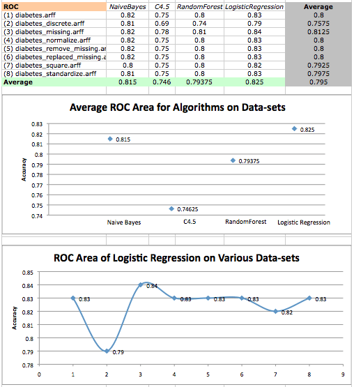
Algorithm ROC area averages on diabetes datasets and a scatterplot of logistic regression performance on various datasets

The results suggests that, once again, LogisticRegression performed the best, while C4.5 performed the worst. On average, it also seems that the dataset corrected for missing values performed the best, while the discrete data set performed the worst.

In both cases, we find that tree algorithms do not perform as well on this dataset. In fact, all results given by C4.5 (and all but one result of RandomForest) have statistically significant differences compared to those results given by LogisticRegression.

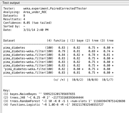
Weka Experimenter output comparing ROC curve area of Logistic Regression with ROC curve area of other algorithms.

This poor performance may be a result of the tree algorithm’s complexity. Measuring relationship with dependent and independent variables may be an advantage here. Also, C4.5 may not be choosing the correct attribute for its analysis, and therefore worsening predictions based on highest information gain.

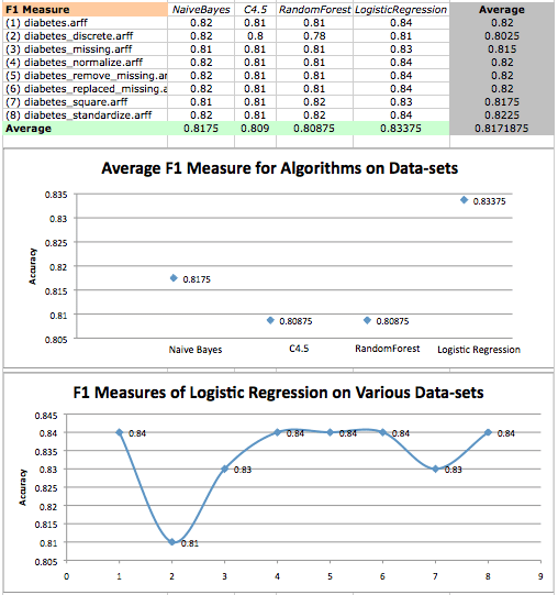
F1 Measure values on diabetes datasets and a scatterplot of logistic regression F1 measures on various datasets.

In the first two analyses, we found that the performance of Naive Bayes followed closely behind the performance of LogisticRegression. Now we find that all but one result of Naive Bayes have a statistically significant difference compared to results given by LogisticRegression.

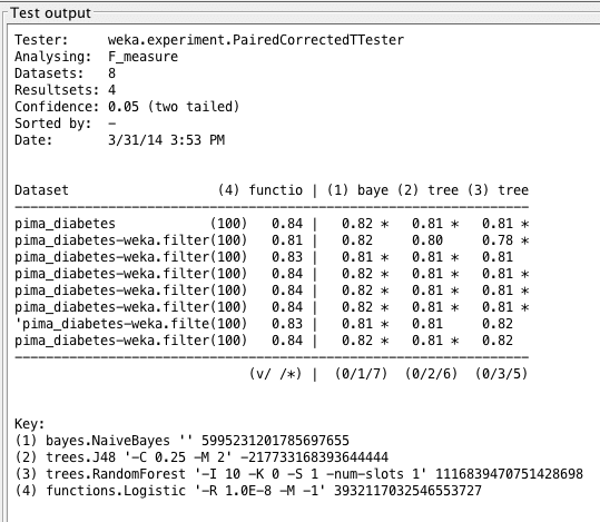
Weka Experimenter output comparing F1 score of Logistic Regression with F1 scores of other algorithms.

The results show us that LogisticRegression performs best, but not by much. This means that LogisticRegression has the most accurate tests in this case, and it learns quite well on this dataset. Just to recall the computation behind the F1-measure, we know:

• Recall: R = TP / (TP + FN),
• Precision: P = TP / (TP + FP), and
• F1-Measure: F1 = 2[ (R * P) / (R + P) ],

where TP = True Positive, FP = False Positive, FN = False Negative.

Our results then suggest that LogisticRegression maximizes the rate of True Positives, and minimizes the rate of False Negatives and False Positives. As for poor performance, I am led to believe that the predictions done by Naive Bayes are just too “naive” and the algorithm therefore uses independence too liberally.

We may need more data to provide more evidence for a particular event occurring, which should better support its prediction. Tree algorithms in this case may suffer due to their complexity, or just because of choosing incorrect attributes for analysis. This may become less of a problem with larger datasets.

Interestingly enough, we also find that the best performing algorithm, LogisticRegression, performs the worst on the diabetes_discrete.arff dataset. It’s probably safe to assume that, for LogisticRegression, all transforms of the data (except for diabetes_discrete.arff) seem to yield better very similar results, and this is very clear through the similar trend in each scatterplot!

Next up in Part 3 we will investigate improvements to the classification accuracy and final presentation of results.

Discover Machine Learning Without The Code!

Develop Your Own Models in Minutes

...with just a few a few clicks

Discover how in my new Ebook:
Machine Learning Mastery With Weka

Covers self-study tutorials and end-to-end projects like:
Loading data, visualization, build models, tuning, and much more...

Finally Bring The Machine Learning To Your Own Projects

Skip the Academics. Just Results.

See What's Inside