Simulated Annealing is a stochastic global search optimization algorithm.
This means that it makes use of randomness as part of the search process. This makes the algorithm appropriate for nonlinear objective functions where other local search algorithms do not operate well.
Like the stochastic hill climbing local search algorithm, it modifies a single solution and searches the relatively local area of the search space until the local optima is located. Unlike the hill climbing algorithm, it may accept worse solutions as the current working solution.
The likelihood of accepting worse solutions starts high at the beginning of the search and decreases with the progress of the search, giving the algorithm the opportunity to first locate the region for the global optima, escaping local optima, then hill climb to the optima itself.
In this tutorial, you will discover the simulated annealing optimization algorithm for function optimization.
After completing this tutorial, you will know:
Simulated annealing is a stochastic global search algorithm for function optimization.
How to implement the simulated annealing algorithm from scratch in Python.
How to use the simulated annealing algorithm and inspect the results of the algorithm.
Let’s get started.
Simulated Annealing From Scratch in Python Photo by Susanne Nilsson, some rights reserved.
Tutorial Overview
This tutorial is divided into three parts; they are:
The algorithm is inspired by annealing in metallurgy where metal is heated to a high temperature quickly, then cooled slowly, which increases its strength and makes it easier to work with.
The annealing process works by first exciting the atoms in the material at a high temperature, allowing the atoms to move around a lot, then decreasing their excitement slowly, allowing the atoms to fall into a new, more stable configuration.
When hot, the atoms in the material are more free to move around, and, through random motion, tend to settle into better positions. A slow cooling brings the material to an ordered, crystalline state.
The simulated annealing optimization algorithm can be thought of as a modified version of stochastic hill climbing.
Stochastic hill climbing maintains a single candidate solution and takes steps of a random but constrained size from the candidate in the search space. If the new point is better than the current point, then the current point is replaced with the new point. This process continues for a fixed number of iterations.
Simulated annealing executes the search in the same way. The main difference is that new points that are not as good as the current point (worse points) are accepted sometimes.
A worse point is accepted probabilistically where the likelihood of accepting a solution worse than the current solution is a function of the temperature of the search and how much worse the solution is than the current solution.
The algorithm varies from Hill-Climbing in its decision of when to replace S, the original candidate solution, with R, its newly tweaked child. Specifically: if R is better than S, we’ll always replace S with R as usual. But if R is worse than S, we may still replace S with R with a certain probability
The initial temperature for the search is provided as a hyperparameter and decreases with the progress of the search. A number of different schemes (annealing schedules) may be used to decrease the temperature during the search from the initial value to a very low value, although it is common to calculate temperature as a function of the iteration number.
A popular example for calculating temperature is the so-called “fast simulated annealing,” calculated as follows
temperature = initial_temperature / (iteration_number + 1)
We add one to the iteration number in the case that iteration numbers start at zero, to avoid a divide by zero error.
The acceptance of worse solutions uses the temperature as well as the difference between the objective function evaluation of the worse solution and the current solution. A value is calculated between 0 and 1 using this information, indicating the likelihood of accepting the worse solution. This distribution is then sampled using a random number, which, if less than the value, means the worse solution is accepted.
It is this acceptance probability, known as the Metropolis criterion, that allows the algorithm to escape from local minima when the temperature is high.
Where exp() is e (the mathematical constant) raised to a power of the provided argument, and objective(new), and objective(current) are the objective function evaluation of the new (worse) and current candidate solutions.
The effect is that poor solutions have more chances of being accepted early in the search and less likely of being accepted later in the search. The intent is that the high temperature at the beginning of the search will help the search locate the basin for the global optima and the low temperature later in the search will help the algorithm hone in on the global optima.
The temperature starts high, allowing the process to freely move about the search space, with the hope that in this phase the process will find a good region with the best local minimum. The temperature is then slowly brought down, reducing the stochasticity and forcing the search to converge to a minimum
Now that we are familiar with the simulated annealing algorithm, let’s look at how to implement it from scratch.
Want to Get Started With Optimization Algorithms?
Take my free 7-day email crash course now (with sample code).
Click to sign-up and also get a free PDF Ebook version of the course.
Implement Simulated Annealing
In this section, we will explore how we might implement the simulated annealing optimization algorithm from scratch.
First, we must define our objective function and the bounds on each input variable to the objective function. The objective function is just a Python function we will name objective(). The bounds will be a 2D array with one dimension for each input variable that defines the minimum and maximum for the variable.
For example, a one-dimensional objective function and bounds would be defined as follows:
1
2
3
4
5
6
# objective function
def objective(x):
return0
# define range for input
bounds=asarray([[-5.0,5.0]])
Next, we can generate our initial point as a random point within the bounds of the problem, then evaluate it using the objective function.
We need to maintain the “current” solution that is the focus of the search and that may be replaced with better solutions.
1
2
3
...
# current working solution
curr,curr_eval=best,best_eval
Now we can loop over a predefined number of iterations of the algorithm defined as “n_iterations“, such as 100 or 1,000.
1
2
3
4
...
# run the algorithm
foriinrange(n_iterations):
...
The first step of the algorithm iteration is to generate a new candidate solution from the current working solution, e.g. take a step.
This requires a predefined “step_size” parameter, which is relative to the bounds of the search space. We will take a random step with a Gaussian distribution where the mean is our current point and the standard deviation is defined by the “step_size“. That means that about 99 percent of the steps taken will be within 3 * step_size of the current point.
1
2
3
...
# take a step
candidate=solution+randn(len(bounds))*step_size
We don’t have to take steps in this way. You may wish to use a uniform distribution between 0 and the step size. For example:
1
2
3
...
# take a step
candidate=solution+rand(len(bounds))*step_size
Next, we need to evaluate it.
1
2
3
...
# evaluate candidate point
candidate_eval=objective(candidate)
We then need to check if the evaluation of this new point is as good as or better than the current best point, and if it is, replace our current best point with this new point.
This is separate from the current working solution that is the focus of the search.
1
2
3
4
5
6
7
...
# check for new best solution
ifcandidate_eval<best_eval:
# store new best point
best,best_eval=candidate,candidate_eval
# report progress
print('>%d f(%s) = %.5f'%(i,best,best_eval))
Next, we need to prepare to replace the current working solution.
The first step is to calculate the difference between the objective function evaluation of the current solution and the current working solution.
1
2
3
...
# difference between candidate and current point evaluation
diff=candidate_eval-curr_eval
Next, we need to calculate the current temperature, using the fast annealing schedule, where “temp” is the initial temperature provided as an argument.
1
2
3
...
# calculate temperature for current epoch
t=temp/float(i+1)
We can then calculate the likelihood of accepting a solution with worse performance than our current working solution.
1
2
3
...
# calculate metropolis acceptance criterion
metropolis=exp(-diff/t)
Finally, we can accept the new point as the current working solution if it has a better objective function evaluation (the difference is negative) or if the objective function is worse, but we probabilistically decide to accept it.
1
2
3
4
5
...
# check if we should keep the new point
ifdiff<0orrand()<metropolis:
# store the new current point
curr,curr_eval=candidate,candidate_eval
And that’s it.
We can implement this simulated annealing algorithm as a reusable function that takes the name of the objective function, the bounds of each input variable, the total iterations, step size, and initial temperature as arguments, and returns the best solution found and its evaluation.
# difference between candidate and current point evaluation
diff=candidate_eval-curr_eval
# calculate temperature for current epoch
t=temp/float(i+1)
# calculate metropolis acceptance criterion
metropolis=exp(-diff/t)
# check if we should keep the new point
ifdiff<0orrand()<metropolis:
# store the new current point
curr,curr_eval=candidate,candidate_eval
return[best,best_eval]
Now that we know how to implement the simulated annealing algorithm in Python, let’s look at how we might use it to optimize an objective function.
Simulated Annealing Worked Example
In this section, we will apply the simulated annealing optimization algorithm to an objective function.
First, let’s define our objective function.
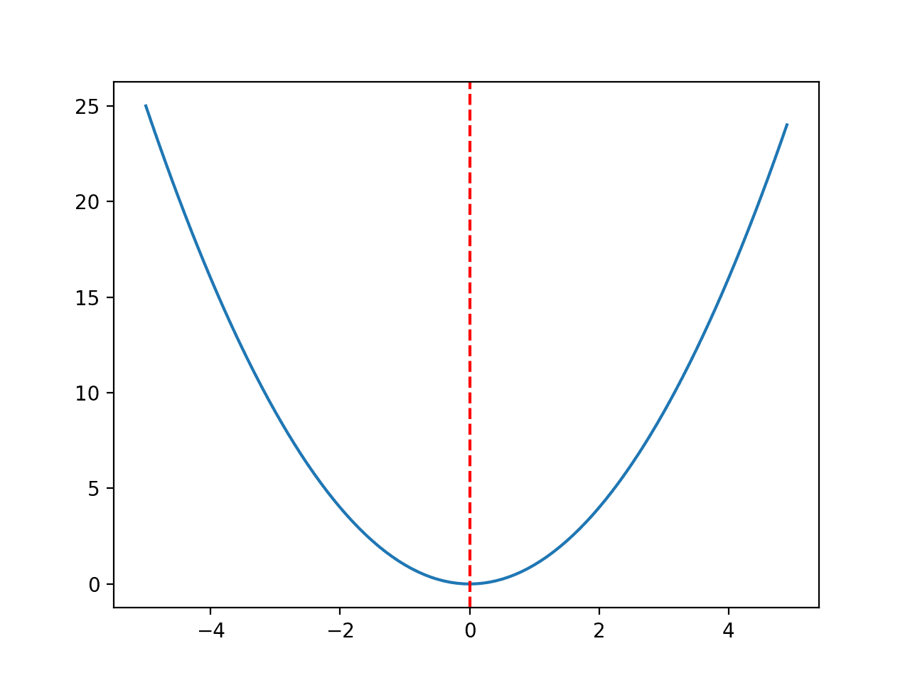
We will use a simple one-dimensional x^2 objective function with the bounds [-5, 5].
The example below defines the function, then creates a line plot of the response surface of the function for a grid of input values, and marks the optima at f(0.0) = 0.0 with a red line
1
2
3
4
5
6
7
8
9
10
11
12
13
14
15
16
17
18
19
20
21
22
# convex unimodal optimization function
from numpy import arange
from matplotlib import pyplot
# objective function
def objective(x):
returnx[0]**2.0
# define range for input
r_min,r_max=-5.0,5.0
# sample input range uniformly at 0.1 increments
inputs=arange(r_min,r_max,0.1)
# compute targets
results=[objective([x])forxininputs]
# create a line plot of input vs result
pyplot.plot(inputs,results)
# define optimal input value
x_optima=0.0
# draw a vertical line at the optimal input
pyplot.axvline(x=x_optima,ls='--',color='red')
# show the plot
pyplot.show()
Running the example creates a line plot of the objective function and clearly marks the function optima.
Line Plot of Objective Function With Optima Marked With a Dashed Red Line
Before we apply the optimization algorithm to the problem, let’s take a moment to understand the acceptance criterion a little better.
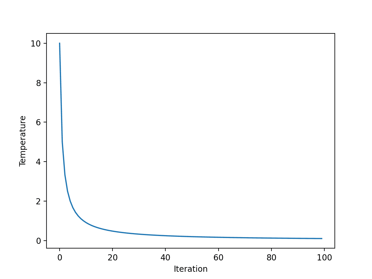
First, the fast annealing schedule is an exponential function of the number of iterations. We can make this clear by creating a plot of the temperature for each algorithm iteration.
We will use an initial temperature of 10 and 100 algorithm iterations, both arbitrarily chosen.
The complete example is listed below.
1
2
3
4
5
6
7
8
9
10
11
12
13
14
15
# explore temperature vs algorithm iteration for simulated annealing
Running the example calculates the temperature for each algorithm iteration and creates a plot of algorithm iteration (x-axis) vs. temperature (y-axis).
We can see that temperature drops rapidly, exponentially, not linearly, such that after 20 iterations it is below 1 and stays low for the remainder of the search.
Line Plot of Temperature vs. Algorithm Iteration for Fast Annealing
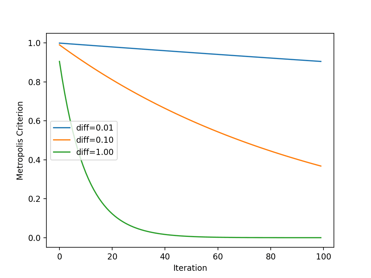
Next, we can get a better idea of how the metropolis acceptance criterion changes over time with the temperature.
Recall that the criterion is a function of temperature, but is also a function of how different the objective evaluation of the new point is compared to the current working solution. As such, we will plot the criterion for a few different “differences in objective function value” to see the effect it has on acceptance probability.
The complete example is listed below.
1
2
3
4
5
6
7
8
9
10
11
12
13
14
15
16
17
18
19
20
21
22
23
# explore metropolis acceptance criterion for simulated annealing
Running the example calculates the metropolis acceptance criterion for each algorithm iteration using the temperature shown for each iteration (shown in the previous section).
The plot has three lines for three differences between the new worse solution and the current working solution.
We can see that the worse the solution is (the larger the difference), the less likely the model is to accept the worse solution regardless of the algorithm iteration, as we might expect. We can also see that in all cases, the likelihood of accepting worse solutions decreases with algorithm iteration.
Line Plot of Metropolis Acceptance Criterion vs. Algorithm Iteration for Simulated Annealing
Now that we are more familiar with the behavior of the temperature and metropolis acceptance criterion over time, let’s apply simulated annealing to our test problem.
First, we will seed the pseudorandom number generator.
This is not required in general, but in this case, I want to ensure we get the same results (same sequence of random numbers) each time we run the algorithm so we can plot the results later.
1
2
3
...
# seed the pseudorandom number generator
seed(1)
Next, we can define the configuration of the search.
In this case, we will search for 1,000 iterations of the algorithm and use a step size of 0.1. Given that we are using a Gaussian function for generating the step, this means that about 99 percent of all steps taken will be within a distance of (0.1 * 3) of a given point, e.g. three standard deviations.
We will also use an initial temperature of 10.0. The search procedure is more sensitive to the annealing schedule than the initial temperature, as such, initial temperature values are almost arbitrary.
1
2
3
4
5
6
...
n_iterations=1000
# define the maximum step size
step_size=0.1
# initial temperature
temp=10
Next, we can perform the search and report the results.
Running the example reports the progress of the search including the iteration number, the input to the function, and the response from the objective function each time an improvement was detected.
At the end of the search, the best solution is found and its evaluation is reported.
Note: Your results may vary given the stochastic nature of the algorithm or evaluation procedure, or differences in numerical precision. Consider running the example a few times and compare the average outcome.
In this case, we can see about 20 improvements over the 1,000 iterations of the algorithm and a solution that is very close to the optimal input of 0.0 that evaluates to f(0.0) = 0.0.
1
2
3
4
5
6
7
8
9
10
11
12
13
14
15
16
17
18
19
20
21
22
>34 f([-0.78753544]) = 0.62021
>35 f([-0.76914239]) = 0.59158
>37 f([-0.68574854]) = 0.47025
>39 f([-0.64797564]) = 0.41987
>40 f([-0.58914623]) = 0.34709
>41 f([-0.55446029]) = 0.30743
>42 f([-0.41775702]) = 0.17452
>43 f([-0.35038542]) = 0.12277
>50 f([-0.15799045]) = 0.02496
>66 f([-0.11089772]) = 0.01230
>67 f([-0.09238208]) = 0.00853
>72 f([-0.09145261]) = 0.00836
>75 f([-0.05129162]) = 0.00263
>93 f([-0.02854417]) = 0.00081
>144 f([0.00864136]) = 0.00007
>149 f([0.00753953]) = 0.00006
>167 f([-0.00640394]) = 0.00004
>225 f([-0.00044965]) = 0.00000
>503 f([-0.00036261]) = 0.00000
>512 f([0.00013605]) = 0.00000
Done!
f([0.00013605]) = 0.000000
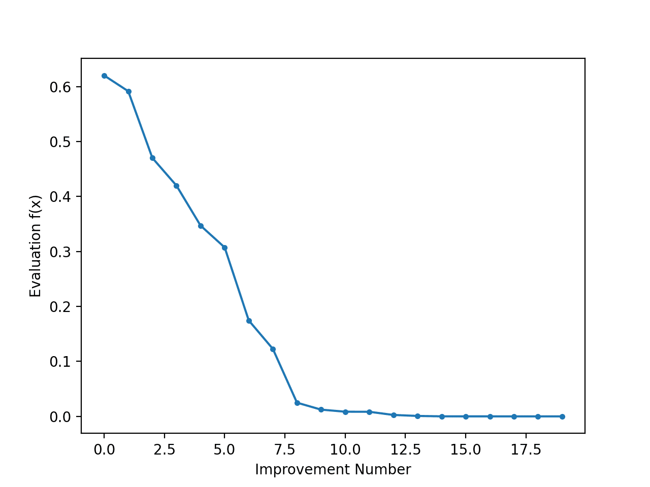
It can be interesting to review the progress of the search as a line plot that shows the change in the evaluation of the best solution each time there is an improvement.
We can update the simulated_annealing() to keep track of the objective function evaluations each time there is an improvement and return this list of scores.
# difference between candidate and current point evaluation
diff=candidate_eval-curr_eval
# calculate temperature for current epoch
t=temp/float(i+1)
# calculate metropolis acceptance criterion
metropolis=exp(-diff/t)
# check if we should keep the new point
ifdiff<0orrand()<metropolis:
# store the new current point
curr,curr_eval=candidate,candidate_eval
return[best,best_eval,scores]
We can then create a line plot of these scores to see the relative change in objective function for each improvement found during the search.
1
2
3
4
5
6
...
# line plot of best scores
pyplot.plot(scores,'.-')
pyplot.xlabel('Improvement Number')
pyplot.ylabel('Evaluation f(x)')
pyplot.show()
Tying this together, the complete example of performing the search and plotting the objective function scores of the improved solutions during the search is listed below.
1
2
3
4
5
6
7
8
9
10
11
12
13
14
15
16
17
18
19
20
21
22
23
24
25
26
27
28
29
30
31
32
33
34
35
36
37
38
39
40
41
42
43
44
45
46
47
48
49
50
51
52
53
54
55
56
57
58
59
60
61
62
63
64
65
66
# simulated annealing search of a one-dimensional objective function
Running the example performs the search and reports the results as before.
A line plot is created showing the objective function evaluation for each improvement during the hill climbing search. We can see about 20 changes to the objective function evaluation during the search with large changes initially and very small to imperceptible changes towards the end of the search as the algorithm converged on the optima.
Line Plot of Objective Function Evaluation for Each Improvement During the Simulated Annealing Search
Further Reading
This section provides more resources on the topic if you are looking to go deeper.
It provides self-study tutorials with full working code on: Gradient Descent, Genetic Algorithms, Hill Climbing, Curve Fitting, RMSProp, Adam,
and much more...
Bring Modern Optimization Algorithms to Your Machine Learning Projects
I went through your tutorial (great info by the way, I’m learning…)and was 99.5% correct on everything till the very end?
Which is that my output for “best and score” is single data point (f([1.96469186]) = 3.0000).
I’m not getting the line plot you did at the very
End? Did you have to change the object function to something different than in your tutorial? My plot for “scores” is empty?
No need to reply, I ended up copying your script over and it worked as advertised? I’m not sure where mine went wrong but its very similar with the exception of some lines of the code are written in different cells?
Excellent tutorial by the way and thank you for sharing…
No Jason, I use Jupyter notebooks, not the command line? My problem was some indentation errors and the fact that I was experimenting with some of your initial values and never returned them back to normal. Lesson learned…Hopefully 😉
You recommend Anaconda for working with machine language programs and I really want to be hands-on in learning it.
I’m worried that it might not work with my system: I have a 32-bit Windows 7 OS (service pack 1) running in my 2GB-memory laptop.
But, there is an Anaconda package that can run for my laptop, right?
By the way, are both Anaconda and PyTorch the same?
Furthermore, which one of your books has the section on how to convert a Windows text file into csv format?
Also, does one of your books also have a section there (along with Python source code) that can help store a data file into an array having the following info in it? (Like the one below…)
20,20,21,1,1,7
7,7,1,1,21,20
21,21,20,1,7,20
7,7,7,7,7,1
1.) You can try miniconda if you believe the Anaconda program is too large. Its a smaller bootstrap version Anaconda.
2.) Anaconda and PyTorch are not the same.
–Anaconda is built off of python
–PyTorch is developed by Facebook AI Research Lab and written in Python, C++, and
CUDA
3.) If you want to learn more about arrays I highly recommend you visit the Numpy.org
–They have tutorials, examples, and a variety of ways to manipulate arrays
_”Furthermore, which one of your books has the section on how to convert a Windows text file into csv format?”_
A text file containing values separated by commas is already a csv format file (to a decent approximation).
Your example data could be stored in an array in a number of ways – for example, look up genfromtxt from numpy to make an array from either a text file or a csv file, per your first question.
Hi Jason ,
Thank you very much for your information, I have been looking for a while of information about this and I have not found much … a query by chance you will have an example of optimization of objective function with restrictions such as the vehicle routing problem (vrp)
I’m supposed to enter an equation with 2 or more unknown and use simulated annealing to find the values of these variables in which the equation becomes = to 0 so can you please help me
Dear, I used this code for my problem it’s not giving me a correct answer.
I tried to change the stepsize and Temp value if I increase the stepsize then the new candidate will go outside from my bound. but in tried hit and trail values for temp and stepsize, i did not get an optimal value
No that’s not a reason. I used a scipy library for the simulated annealing method and its works very well. I also changed an objective function “eggholder equation” its also not working in your implementation but work very well in scipy
Mr. Jason, I need to implement this algorithm to choose best values of hyperparameter alpha, beta and number of topics with best coherence but I do not have an idea to do it. can you help me please?
If you have the function well-defined, you may try using the same algorithm here. But simulated annealing highly dependent on the initial value if your function is not convex.
Thanks Jason, nice article! Adapting the code for my multivariate objective function was a breeze.
Does the Ebook elaborate a bit on choosing step size, Gaussian vs uniform distribution for new candidates, convergence, etc? In other words do you provide practical information in the book to tweak the algorithm to the function?
Is there no information in the book about Monte Carlo?
Btw, in your code only the initial point is limited to the defined bounds, candidates of following iterations are not limited in range.


Hi Jason,
I went through your tutorial (great info by the way, I’m learning…)and was 99.5% correct on everything till the very end?
Which is that my output for “best and score” is single data point (f([1.96469186]) = 3.0000).
I’m not getting the line plot you did at the very
End? Did you have to change the object function to something different than in your tutorial? My plot for “scores” is empty?
No need to reply, I ended up copying your script over and it worked as advertised? I’m not sure where mine went wrong but its very similar with the exception of some lines of the code are written in different cells?
Excellent tutorial by the way and thank you for sharing…
Ron
Well done for getting there!
Sorry to hear that, are you running from the command line?
https://machinelearningmastery.com/faq/single-faq/how-do-i-run-a-script-from-the-command-line
No Jason, I use Jupyter notebooks, not the command line? My problem was some indentation errors and the fact that I was experimenting with some of your initial values and never returned them back to normal. Lesson learned…Hopefully 😉
This will help you copy code without indentation errors:
https://machinelearningmastery.com/faq/single-faq/how-do-i-copy-code-from-a-tutorial
Jason, I think that the indentation in your snippets are messed up.
Thanks, I will investigate.
You recommend Anaconda for working with machine language programs and I really want to be hands-on in learning it.
I’m worried that it might not work with my system: I have a 32-bit Windows 7 OS (service pack 1) running in my 2GB-memory laptop.
But, there is an Anaconda package that can run for my laptop, right?
By the way, are both Anaconda and PyTorch the same?
Furthermore, which one of your books has the section on how to convert a Windows text file into csv format?
Also, does one of your books also have a section there (along with Python source code) that can help store a data file into an array having the following info in it? (Like the one below…)
20,20,21,1,1,7
7,7,1,1,21,20
21,21,20,1,7,20
7,7,7,7,7,1
Francis,
1.) You can try miniconda if you believe the Anaconda program is too large. Its a smaller bootstrap version Anaconda.
2.) Anaconda and PyTorch are not the same.
–Anaconda is built off of python
–PyTorch is developed by Facebook AI Research Lab and written in Python, C++, and
CUDA
3.) If you want to learn more about arrays I highly recommend you visit the Numpy.org
–They have tutorials, examples, and a variety of ways to manipulate arrays
Hope this helps you on your quest.
Ron
Great tips Ron!
Maybe try installing Python in an alternate way?
This will help you load a file:
https://machinelearningmastery.com/load-machine-learning-data-python/
This will help you save the results:
https://machinelearningmastery.com/how-to-save-a-numpy-array-to-file-for-machine-learning/
_”Furthermore, which one of your books has the section on how to convert a Windows text file into csv format?”_
A text file containing values separated by commas is already a csv format file (to a decent approximation).
Your example data could be stored in an array in a number of ways – for example, look up genfromtxt from numpy to make an array from either a text file or a csv file, per your first question.
Cheers!
Data is almost always in CSV format or can easily be converted to CSV format.
You can load CSV files in Python as follows:
https://machinelearningmastery.com/load-machine-learning-data-python/
Hey Jason, love your work, there is a tiny typo in one of the code frags:
candidte_eval = objective(candidate)Thanks! Fixed.
Hi Jason ,
Thank you very much for your information, I have been looking for a while of information about this and I have not found much … a query by chance you will have an example of optimization of objective function with restrictions such as the vehicle routing problem (vrp)
thanks Jason
You’re welcome.
Great suggestion, thanks!
how can i run it with multiple variables can someone help please
What problem are you having exactly?
I need to make this work with 7 variables but I can’t add the number of variables please help me
Why? What is the problem exactly?
I’m supposed to enter an equation with 2 or more unknown and use simulated annealing to find the values of these variables in which the equation becomes = to 0 so can you please help me
I recommend you start by defining a function that takes the unknowns and evaluates your equation using the input values.
You can then configure an optimization algorithm to search for values testing against your objective function.
If this still sounds too challenging, perhaps discuss with your teacher.
But when I try to add an extra variable say y the error is index 1 is out of bounds for axis with size 1 and best_eval = objective (best)
Well I think i might fail this class but hey at least I gave it a try thanks for taking the time to reply great work you have here
Dear, I used this code for my problem it’s not giving me a correct answer.
I tried to change the stepsize and Temp value if I increase the stepsize then the new candidate will go outside from my bound. but in tried hit and trail values for temp and stepsize, i did not get an optimal value
Perhaps the algorithm is not appropriate for your problem?
No that’s not a reason. I used a scipy library for the simulated annealing method and its works very well. I also changed an objective function “eggholder equation” its also not working in your implementation but work very well in scipy
Perhaps the above implementation is too simple and requires modification for your new problem.
Yes maybe, because I used your GA method as well and its work very well but not this one (your implementation) but annealing works from scipy
Mr. Jason, I would like to ask, if we want to use this code for C language, what kind of content need to include ?
You will have to rewrite it in C from scratch.
Mr. Jason, I need to implement this algorithm to choose best values of hyperparameter alpha, beta and number of topics with best coherence but I do not have an idea to do it. can you help me please?
Sure, what problem are you having exactly (i.e. I don’t have the capacity to adapt the code for you)?
I need to run it with two variables, and the objective function is coherence value. thanks for taking the time to reply
If you have the function well-defined, you may try using the same algorithm here. But simulated annealing highly dependent on the initial value if your function is not convex.
Thanks Jason, nice article! Adapting the code for my multivariate objective function was a breeze.
Does the Ebook elaborate a bit on choosing step size, Gaussian vs uniform distribution for new candidates, convergence, etc? In other words do you provide practical information in the book to tweak the algorithm to the function?
Is there no information in the book about Monte Carlo?
Btw, in your code only the initial point is limited to the defined bounds, candidates of following iterations are not limited in range.
Thank you Arnaud for the kind words! The following provides information on all of our ebooks:
https://machinelearningmastery.com/products/
I need to implement this algorithm to choose best values of hyperparameter (gamma, sigma) for LS-SVM model
i need a code for that !
Hi boumeftah…for this purpose, I would recommend investigation of Bayesian Optimization:
https://towardsdatascience.com/a-conceptual-explanation-of-bayesian-model-based-hyperparameter-optimization-for-machine-learning-b8172278050f