Dual Annealing is a stochastic global optimization algorithm.
It is an implementation of the generalized simulated annealing algorithm, an extension of simulated annealing. In addition, it is paired with a local search algorithm that is automatically performed at the end of the simulated annealing procedure.
This combination of effective global and local search procedures provides a powerful algorithm for challenging nonlinear optimization problems.
In this tutorial, you will discover the dual annealing global optimization algorithm.
After completing this tutorial, you will know:
- Dual annealing optimization is a global optimization that is a modified version of simulated annealing that also makes use of a local search algorithm.
- How to use the dual annealing optimization algorithm API in python.
- Examples of using dual annealing to solve global optimization problems with multiple optima.
Kick-start your project with my new book Optimization for Machine Learning, including step-by-step tutorials and the Python source code files for all examples.
Let’s get started.
Dual Annealing Optimization With Python
Photos by Susanne Nilsson, some rights reserved.
Tutorial Overview
This tutorial is divided into three parts; they are:
- What Is Dual Annealing
- Dual Annealing API
- Dual Annealing Example
What Is Dual Annealing
Dual Annealing is a global optimization algorithm.
As such, it is designed for objective functions that have a nonlinear response surface. It is a stochastic optimization algorithm, meaning that it makes use of randomness during the search process and each run of the search may find a different solution.
Dual Annealing is based on the Simulated Annealing optimization algorithm.
Simulated Annealing is a type of stochastic hill climbing where a candidate solution is modified in a random way and the modified solutions are accepted to replace the current candidate solution probabilistically. This means that it is possible for worse solutions to replace the current candidate solution. The probability of this type of replacement is high at the beginning of the search and decreases with each iteration, controlled by the “temperature” hyperparameter.
Dual annealing is an implementation of the classical simulated annealing (CSA) algorithm. It is based on the generalized simulated annealing (GSA) algorithm described in the 1997 paper “Generalized Simulated Annealing Algorithm and Its Application to the Thomson Model.”
It combines the annealing schedule (rate at which the temperature decreases over algorithm iterations) from “fast simulated annealing” (FSA) and the probabilistic acceptance of an alternate statistical procedure “Tsallis statistics” named for the author.
Experimental results find that this generalized simulated annealing algorithm appears to perform better than the classical or the fast versions of the algorithm to which it was compared.
GSA not only converges faster than FSA and CSA, but also has the ability to escape from a local minimum more easily than FSA and CSA.
— Generalized Simulated Annealing for Global Optimization: The GenSA Package, 2013.
In addition to these modifications of simulated annealing, a local search algorithm can be applied to the solution found by the simulated annealing search.
This is desirable as global search algorithms are often good at locating the basin (area in the search space) for the optimal solution but are often poor at finding the most optimal solution in the basin. Whereas local search algorithms excel at finding the optima of a basin.
Pairing a local search with the simulated annealing procedure ensures the search gets the most out of the candidate solution that is located.
Now that we are familiar with the dual annealing algorithm from a high level, let’s look at the API for dual annealing in Python.
Want to Get Started With Optimization Algorithms?
Take my free 7-day email crash course now (with sample code).
Click to sign-up and also get a free PDF Ebook version of the course.
Dual Annealing API
The Dual Annealing global optimization algorithm is available in Python via the dual_annealing() SciPy function.
The function takes the name of the objective function and the bounds of each input variable as minimum arguments for the search.
|
1 2 3 |
... # perform the dual annealing search result = dual_annealing(objective, bounds) |
There are a number of additional hyperparameters for the search that have default values, although you can configure them to customize the search.
The “maxiter” argument specifies the total number of iterations of the algorithm (not the total number of function evaluations) and defaults to 1,000 iterations. The “maxfun” can be specified if desired to limit the total number of function evaluations and defaults to 10 million.
The initial temperature of the search is specified by the “initial_temp” argument, which defaults to 5,230. The annealing process will be restarted once the temperature reaches a value equal to or less than (initial_temp * restart_temp_ratio). The ratio defaults to a very small number 2e-05 (i.e. 0.00002), so the default trigger for re-annealing is a temperature of (5230 * 0.00002) or 0.1046.
The algorithm also provides control over hyperparameters specific to the generalized simulated annealing on which it is based. This includes how far jumps can be made during the search via the “visit” argument, which defaults to 2.62 (values less than 3 are preferred), and the “accept” argument that controls the likelihood of accepting new solutions, which defaults to -5.
The minimize() function is called for the local search with default hyperparameters. The local search can be configured by providing a dictionary of hyperparameter names and values to the “local_search_options” argument.
The local search component of the search can be disabled by setting the “no_local_search” argument to True.
The result of the search is an OptimizeResult object where properties can be accessed like a dictionary. The success (or not) of the search can be accessed via the ‘success‘ or ‘message’ key.
The total number of function evaluations can be accessed via ‘nfev‘ and the optimal input found for the search is accessible via the ‘x‘ key.
Now that we are familiar with the dual annealing API in Python, let’s look at some worked examples.
Dual Annealing Example
In this section, we will look at an example of using the dual annealing algorithm on a multi-modal objective function.
The Ackley function is an example of a multimodal objective function that has a single global optima and multiple local optima in which a local search might get stuck.
As such, a global optimization technique is required. It is a two-dimensional objective function that has a global optima at [0,0], which evaluates to 0.0.
The example below implements the Ackley and creates a three-dimensional surface plot showing the global optima and multiple local optima.
|
1 2 3 4 5 6 7 8 9 10 11 12 13 14 15 16 17 18 19 20 21 22 23 24 25 26 27 28 29 30 |
# ackley multimodal function from numpy import arange from numpy import exp from numpy import sqrt from numpy import cos from numpy import e from numpy import pi from numpy import meshgrid from matplotlib import pyplot from mpl_toolkits.mplot3d import Axes3D # objective function def objective(x, y): return -20.0 * exp(-0.2 * sqrt(0.5 * (x**2 + y**2))) - exp(0.5 * (cos(2 * pi * x) + cos(2 * pi * y))) + e + 20 # define range for input r_min, r_max = -5.0, 5.0 # sample input range uniformly at 0.1 increments xaxis = arange(r_min, r_max, 0.1) yaxis = arange(r_min, r_max, 0.1) # create a mesh from the axis x, y = meshgrid(xaxis, yaxis) # compute targets results = objective(x, y) # create a surface plot with the jet color scheme figure = pyplot.figure() axis = figure.gca(projection='3d') axis.plot_surface(x, y, results, cmap='jet') # show the plot pyplot.show() |
Running the example creates the surface plot of the Ackley function showing the vast number of local optima.
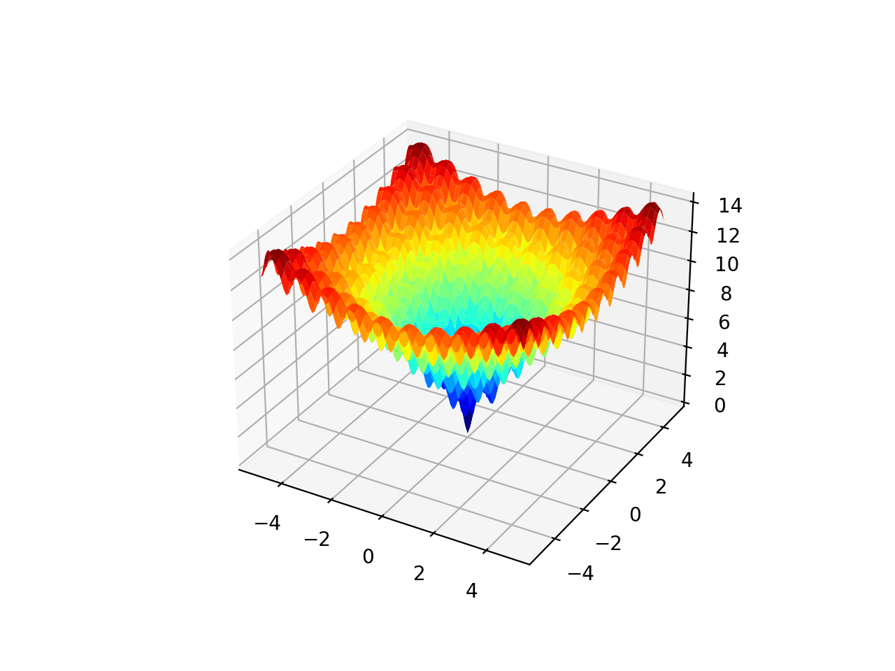
3D Surface Plot of the Ackley Multimodal Function
We can apply the dual annealing algorithm to the Ackley objective function.
First, we can define the bounds of the search space as the limits of the function in each dimension.
|
1 2 3 |
... # define the bounds on the search bounds = [[r_min, r_max], [r_min, r_max]] |
We can then apply the search by specifying the name of the objective function and the bounds of the search.
In this case, we will use the default hyperparameters.
|
1 2 3 |
... # perform the simulated annealing search result = dual_annealing(objective, bounds) |
After the search is complete, it will report the status of the search and the number of iterations performed, as well as the best result found with its evaluation.
|
1 2 3 4 5 6 7 8 |
... # summarize the result print('Status : %s' % result['message']) print('Total Evaluations: %d' % result['nfev']) # evaluate solution solution = result['x'] evaluation = objective(solution) print('Solution: f(%s) = %.5f' % (solution, evaluation)) |
Tying this together, the complete example of applying dual annealing to the Ackley objective function is listed below.
|
1 2 3 4 5 6 7 8 9 10 11 12 13 14 15 16 17 18 19 20 21 22 23 24 25 26 27 |
# dual annealing global optimization for the ackley multimodal objective function from scipy.optimize import dual_annealing from numpy.random import rand from numpy import exp from numpy import sqrt from numpy import cos from numpy import e from numpy import pi # objective function def objective(v): x, y = v return -20.0 * exp(-0.2 * sqrt(0.5 * (x**2 + y**2))) - exp(0.5 * (cos(2 * pi * x) + cos(2 * pi * y))) + e + 20 # define range for input r_min, r_max = -5.0, 5.0 # define the bounds on the search bounds = [[r_min, r_max], [r_min, r_max]] # perform the dual annealing search result = dual_annealing(objective, bounds) # summarize the result print('Status : %s' % result['message']) print('Total Evaluations: %d' % result['nfev']) # evaluate solution solution = result['x'] evaluation = objective(solution) print('Solution: f(%s) = %.5f' % (solution, evaluation)) |
Running the example executes the optimization, then reports the results.
Note: Your results may vary given the stochastic nature of the algorithm or evaluation procedure, or differences in numerical precision. Consider running the example a few times and compare the average outcome.
In this case, we can see that the algorithm located the optima with inputs very close to zero and an objective function evaluation that is practically zero.
We can see that a total of 4,136 function evaluations were performed.
|
1 2 3 |
Status : ['Maximum number of iteration reached'] Total Evaluations: 4136 Solution: f([-2.26474440e-09 -8.28465933e-09]) = 0.00000 |
Further Reading
This section provides more resources on the topic if you are looking to go deeper.
Papers
- Generalized Simulated Annealing Algorithm and Its Application to the Thomson Model, 1997.
- Generalized simulated annealing, 1996.
- Generalized Simulated Annealing for Global Optimization: The GenSA Package, 2013.
APIs
Articles
Summary
In this tutorial, you discovered the dual annealing global optimization algorithm.
Specifically, you learned:
- Dual annealing optimization is a global optimization that is a modified version of simulated annealing that also makes use of a local search algorithm.
- How to use the dual annealing optimization algorithm API in python.
- Examples of using dual annealing to solve global optimization problems with multiple optima.
Do you have any questions?
Ask your questions in the comments below and I will do my best to answer.
Get a Handle on Modern Optimization Algorithms!
Develop Your Understanding of Optimization
...with just a few lines of python code
Discover how in my new Ebook:
Optimization for Machine Learning
It provides self-study tutorials with full working code on:
Gradient Descent, Genetic Algorithms, Hill Climbing, Curve Fitting, RMSProp, Adam,
and much more...

")


please, could you use it with housing dataset?
Thank you for the suggestion.
Could you please include inequality /equality constraints with multi dimensional input/design variables (more than 3) to arrive Single Objective Optimization?
Thanks for the suggestion.
Thank for the tutorial! I get the following error:
TypeError: objective() missing 1 required positional argument: ‘y’
when I run:
result = dual_annealing(objective, bounds)
I don’t see the error. What version of scikit-learn are you using?
Hi Jason,
This is very helpful. Thanks for sharing! Does dual annealing algorithm works with global constraints? For example, I have 10 products and want to find the optimal price for each to maximize profit, but also don’t want my volume to drop too much. It seems the dual_annealing() api from Python doesn’t have a constraints parameter.
Hi Yw….The following may be of interest to you:
https://aicorespot.io/dual-annealing-optimization-with-python/
Hi Jason,
Thank you for your explanation. I have one question for you, if you wouldn’t mind. What is the termination criterion? You mentioned the default for iteration is 1000, does it mean if I set 10,000, I will have more searches?
I have tried maxiter at 10,000; it searches more and more. If this is true, how does it converge?
Rregards,
Dawit
Hi Dawit…You are very welcome! The following resource may be of interest:
https://lightrun.com/answers/scipy-scipy-enh-stopping-rule-for-dual_annealing-function
Thanks, James. You are the star!