In this post you will discover 4 recipes for linear regression for the R platform.
You can copy and paste the recipes in this post to make a jump-start on your own problem or to learn and practice with linear regression in R.
Kick-start your project with my new book Machine Learning Mastery With R, including step-by-step tutorials and the R source code files for all examples.
Let’s get started.
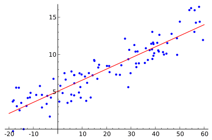
Ordinary Least Squares Regression
Some rights reserved
Each example in this post uses the longley dataset provided in the datasets package that comes with R. The longley dataset describes 7 economic variables observed from 1947 to 1962 used to predict the number of people employed yearly.
Ordinary Least Squares Regression
Ordinary Least Squares (OLS) regression is a linear model that seeks to find a set of coefficients for a line/hyper-plane that minimise the sum of the squared errors.
|
1 2 3 4 5 6 7 8 9 10 11 |
# load data data(longley) # fit model fit <- lm(Employed~., longley) # summarize the fit summary(fit) # make predictions predictions <- predict(fit, longley) # summarize accuracy mse <- mean((longley$Employed - predictions)^2) print(mse) |
Learn more about the lm function and the stats package.
Need more Help with R for Machine Learning?
Take my free 14-day email course and discover how to use R on your project (with sample code).
Click to sign-up and also get a free PDF Ebook version of the course.
Stepwize Linear Regression
Stepwise Linear Regression is a method that makes use of linear regression to discover which subset of attributes in the dataset result in the best performing model. It is step-wise because each iteration of the method makes a change to the set of attributes and creates a model to evaluate the performance of the set.
|
1 2 3 4 5 6 7 8 9 10 11 12 13 14 15 |
# load data data(longley) # fit model base <- lm(Employed~., longley) # summarize the fit summary(base) # perform step-wise feature selection fit <- step(base) # summarize the selected model summary(fit) # make predictions predictions <- predict(fit, longley) # summarize accuracy mse <- mean((longley$Employed - predictions)^2) print(mse) |
Learn more about the step function and the stats package.
Principal Component Regression
Principal Component Regression (PCR) creates a linear regression model using the outputs of a Principal Component Analysis (PCA) to estimate the coefficients of the model. PCR is useful when the data has highly correlated predictors.
|
1 2 3 4 5 6 7 8 9 10 11 12 13 |
# load the package library(pls) # load data data(longley) # fit model fit <- pcr(Employed~., data=longley, validation="CV") # summarize the fit summary(fit) # make predictions predictions <- predict(fit, longley, ncomp=6) # summarize accuracy mse <- mean((longley$Employed - predictions)^2) print(mse) |
Learn more about the pcr function and the pls package.
Partial Least Squares Regression
Partial Least Squares (PLS) Regression creates a linear model of the data in a transformed projection of problem space. Like PCR, PLS is appropriate for data with highly-correlated predictors.
|
1 2 3 4 5 6 7 8 9 10 11 12 13 |
# load the package library(pls) # load data data(longley) # fit model fit <- plsr(Employed~., data=longley, validation="CV") # summarize the fit summary(fit) # make predictions predictions <- predict(fit, longley, ncomp=6) # summarize accuracy mse <- mean((longley$Employed - predictions)^2) print(mse) |
Learn more about the plsr function and the pls package.
Summary
In this post you discovered 4 recipes for creating linear regression models in R and making predictions using those models.
Chapter 6 of Applied Predictive Modeling by Kuhn and Johnson provides an excellent introduction to linear regression with R for beginners. Practical Regression and Anova using R (PDF) by Faraway provides a more in-depth treatment.
Discover Faster Machine Learning in R!
Develop Your Own Models in Minutes
...with just a few lines of R code
Discover how in my new Ebook:
Machine Learning Mastery With R
Covers self-study tutorials and end-to-end projects like:
Loading data, visualization, build models, tuning, and much more...
Finally Bring Machine Learning To Your Own Projects
Skip the Academics. Just Results.


Is there any reason why SLR is not performing better than OLSR? again, the question comes how to judge ‘better’. I notice that rmse(SLR)>rmse(OLSR). If we are aiming for a better fit shouldn’t the rmse decrease?
I think the rmse calculation step missed taking the square root.
rmse <- sqrt( mean((longley$Employed – predictions)^2) )
Yes thank you, this was something I noticed as well and was unsure of.
Jason calculated mse not rmse. So there is no square root.
Anyone , please confirm/oppose my understanding. Are following attributes found best by “Stepwize Linear Regression” algorithm?
GNP + Unemployed + Armed.Forces + Year
We cannot know what algorithm will be best for your data, try a suite of methods and compare the skill of each.
See this post:
https://machinelearningmastery.com/a-data-driven-approach-to-machine-learning/
Sorry, I was not clear. I am not asking which algorithm is best. I am simply running the example code above of ““Stepwize Linear Regression” . Then I am trying to understand the what gets printed on screen. (Thus the data is “longley”. )
I see that three steps/iterations are performed.
My understanding:
1. After the first iteration “GNP.deflator” is discarded because its AIC was lowest(-35.163)
2. After the second iteration “Population” is discarded because its AIC was lowest(-36.799)
3. After 3rd step GNP should be discarded. ( Its AIC is -31.879)
Is my understanding correct?
Ah, I see. The result is the variables suggested or chosen for the final model.