How To Implement Simple Linear Regression From Scratch With Python

By Jason Brownlee on October 26, 2016 in Code Algorithms From Scratch

Last Updated on May 11, 2020

Linear regression is a prediction method that is more than 200 years old.

Simple linear regression is a great first machine learning algorithm to implement as it requires you to estimate properties from your training dataset, but is simple enough for beginners to understand.

In this tutorial, you will discover how to implement the simple linear regression algorithm from scratch in Python.

After completing this tutorial you will know:

How to estimate statistical quantities from training data.
How to estimate linear regression coefficients from data.
How to make predictions using linear regression for new data.

Kick-start your project with my new book Machine Learning Algorithms From Scratch, including step-by-step tutorials and the Python source code files for all examples.

Let’s get started.

Update Aug/2018: Tested and updated to work with Python 3.6.
Update Feb/2019: Minor update to the expected default RMSE for the insurance dataset.

How To Implement Simple Linear Regression From Scratch With Python
Photo by Kamyar Adl, some rights reserved.

Description

This section is divided into two parts, a description of the simple linear regression technique and a description of the dataset to which we will later apply it.

Simple Linear Regression

Linear regression assumes a linear or straight line relationship between the input variables (X) and the single output variable (y).

More specifically, that output (y) can be calculated from a linear combination of the input variables (X). When there is a single input variable, the method is referred to as a simple linear regression.

In simple linear regression we can use statistics on the training data to estimate the coefficients required by the model to make predictions on new data.

The line for a simple linear regression model can be written as:

1	y = b0 + b1 * x

where b0 and b1 are the coefficients we must estimate from the training data.

Once the coefficients are known, we can use this equation to estimate output values for y given new input examples of x.

It requires that you calculate statistical properties from the data such as mean, variance and covariance.

All the algebra has been taken care of and we are left with some arithmetic to implement to estimate the simple linear regression coefficients.

Briefly, we can estimate the coefficients as follows:

1 2	B1 = sum((x(i) - mean(x)) * (y(i) - mean(y))) / sum( (x(i) - mean(x))^2 ) B0 = mean(y) - B1 * mean(x)

where the i refers to the value of the ith value of the input x or output y.

Don’t worry if this is not clear right now, these are the functions will implement in the tutorial.

Swedish Insurance Dataset

We will use a real dataset to demonstrate simple linear regression.

The dataset is called the “Auto Insurance in Sweden” dataset and involves predicting the total payment for all the claims in thousands of Swedish Kronor (y) given the total number of claims (x).

This means that for a new number of claims (x) we will be able to predict the total payment of claims (y).

Here is a small sample of the first 5 records of the dataset.

108,392.5

19,46.2

13,15.7

124,422.2

40,119.4

Using the Zero Rule algorithm (that predicts the mean value) a Root Mean Squared Error or RMSE of about 81 (thousands of Kronor) is expected.

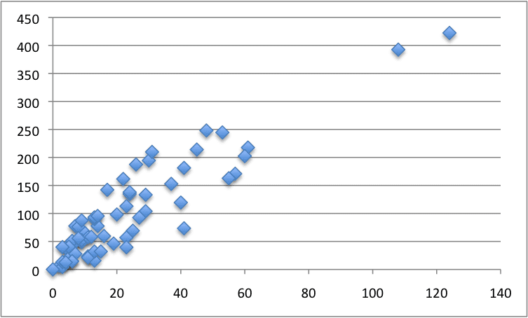
Below is a scatter plot of the entire dataset.

Swedish Insurance Dataset

You can download the raw dataset from here or here.

Save it to a CSV file in your local working directory with the name “insurance.csv“.

Note, you may need to convert the European “,” to the decimal “.”. You will also need change the file from white-space-separated variables to CSV format.

Tutorial

This tutorial is broken down into five parts:

Calculate Mean and Variance.
Calculate Covariance.
Estimate Coefficients.
Make Predictions.
Predict Insurance.

These steps will give you the foundation you need to implement and train simple linear regression models for your own prediction problems.

1. Calculate Mean and Variance

The first step is to estimate the mean and the variance of both the input and output variables from the training data.

The mean of a list of numbers can be calculated as:

1	mean(x) = sum(x) / count(x)

Below is a function named mean() that implements this behavior for a list of numbers.

# Calculate the mean value of a list of numbers

def mean(values):

return sum(values) / float(len(values))

The variance is the sum squared difference for each value from the mean value.

Variance for a list of numbers can be calculated as:

1	variance = sum( (x - mean(x))^2 )

Below is a function named variance() that calculates the sample variance of a list of numbers (Note that we are intentionally calculating the sum squared difference from the mean, instead of the average squared difference from the mean). It requires the mean of the list to be provided as an argument, just so we don’t have to calculate it more than once.

# Calculate the variance of a list of numbers

def variance(values, mean):

return sum([(x-mean)**2 for x in values])

We can put these two functions together and test them on a small contrived dataset.

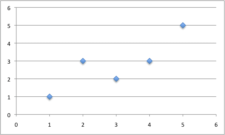
Below is a small dataset of x and y values.

NOTE: delete the column headers from this data if you save it to a .CSV file for use with the final code example.

x, y

1, 1

2, 3

4, 3

3, 2

5, 5

We can plot this dataset on a scatter plot graph as follows:

Small Contrived Dataset For Simple Linear Regression

We can calculate the mean and variance for both the x and y values in the example below.

# Estimate Mean and Variance

# Calculate the mean value of a list of numbers

def mean(values):

return sum(values) / float(len(values))

# Calculate the variance of a list of numbers

def variance(values, mean):

return sum([(x-mean)**2 for x in values])

# calculate mean and variance

dataset = [[1, 1], [2, 3], [4, 3], [3, 2], [5, 5]]

x = [row[0] for row in dataset]

y = [row[1] for row in dataset]

mean_x, mean_y = mean(x), mean(y)

var_x, var_y = variance(x, mean_x), variance(y, mean_y)

print('x stats: mean=%.3f variance=%.3f' % (mean_x, var_x))

print('y stats: mean=%.3f variance=%.3f' % (mean_y, var_y))

Running this example prints out the mean and variance for both columns.

1 2	x stats: mean=3.000 variance=10.000 y stats: mean=2.800 variance=8.800

This is our first step, next we need to put these values to use in calculating the covariance.

2. Calculate Covariance

The covariance of two groups of numbers describes how those numbers change together.

Covariance is a generalization of correlation. Correlation describes the relationship between two groups of numbers, whereas covariance can describe the relationship between two or more groups of numbers.

Additionally, covariance can be normalized to produce a correlation value.

Nevertheless, we can calculate the covariance between two variables as follows:

1	covariance = sum((x(i) - mean(x)) * (y(i) - mean(y)))

Below is a function named covariance() that implements this statistic. It builds upon the previous step and takes the lists of x and y values as well as the mean of these values as arguments.

# Calculate covariance between x and y

def covariance(x, mean_x, y, mean_y):

covar = 0.0

for i in range(len(x)):

covar += (x[i] - mean_x) * (y[i] - mean_y)

return covar

We can test the calculation of the covariance on the same small contrived dataset as in the previous section.

Putting it all together we get the example below.

# Calculate Covariance

# Calculate the mean value of a list of numbers

def mean(values):

return sum(values) / float(len(values))

# Calculate covariance between x and y

def covariance(x, mean_x, y, mean_y):

covar = 0.0

for i in range(len(x)):

covar += (x[i] - mean_x) * (y[i] - mean_y)

return covar

# calculate covariance

dataset = [[1, 1], [2, 3], [4, 3], [3, 2], [5, 5]]

x = [row[0] for row in dataset]

y = [row[1] for row in dataset]

mean_x, mean_y = mean(x), mean(y)

covar = covariance(x, mean_x, y, mean_y)

print('Covariance: %.3f' % (covar))

Running this example prints the covariance for the x and y variables.

1	Covariance: 8.000

We now have all the pieces in place to calculate the coefficients for our model.

3. Estimate Coefficients

We must estimate the values for two coefficients in simple linear regression.

The first is B1 which can be estimated as:

1	B1 = sum((x(i) - mean(x)) * (y(i) - mean(y))) / sum( (x(i) - mean(x))^2 )

We have learned some things above and can simplify this arithmetic to:

1	B1 = covariance(x, y) / variance(x)

We already have functions to calculate covariance() and variance().

Next, we need to estimate a value for B0, also called the intercept as it controls the starting point of the line where it intersects the y-axis.

1	B0 = mean(y) - B1 * mean(x)

Again, we know how to estimate B1 and we have a function to estimate mean().

We can put all of this together into a function named coefficients() that takes the dataset as an argument and returns the coefficients.

# Calculate coefficients

def coefficients(dataset):

x = [row[0] for row in dataset]

y = [row[1] for row in dataset]

x_mean, y_mean = mean(x), mean(y)

b1 = covariance(x, x_mean, y, y_mean) / variance(x, x_mean)

b0 = y_mean - b1 * x_mean

return [b0, b1]

We can put this together with all of the functions from the previous two steps and test out the calculation of coefficients.

# Calculate Coefficients

# Calculate the mean value of a list of numbers

def mean(values):

return sum(values) / float(len(values))

# Calculate covariance between x and y

def covariance(x, mean_x, y, mean_y):

covar = 0.0

for i in range(len(x)):

covar += (x[i] - mean_x) * (y[i] - mean_y)

return covar

# Calculate the variance of a list of numbers

def variance(values, mean):

return sum([(x-mean)**2 for x in values])

# Calculate coefficients

def coefficients(dataset):

x = [row[0] for row in dataset]

y = [row[1] for row in dataset]

x_mean, y_mean = mean(x), mean(y)

b1 = covariance(x, x_mean, y, y_mean) / variance(x, x_mean)

b0 = y_mean - b1 * x_mean

return [b0, b1]

# calculate coefficients

dataset = [[1, 1], [2, 3], [4, 3], [3, 2], [5, 5]]

b0, b1 = coefficients(dataset)

print('Coefficients: B0=%.3f, B1=%.3f' % (b0, b1))

Running this example calculates and prints the coefficients.

1	Coefficients: B0=0.400, B1=0.800

Now that we know how to estimate the coefficients, the next step is to use them.

4. Make Predictions

The simple linear regression model is a line defined by coefficients estimated from training data.

Once the coefficients are estimated, we can use them to make predictions.

The equation to make predictions with a simple linear regression model is as follows:

1	y = b0 + b1 * x

Below is a function named simple_linear_regression() that implements the prediction equation to make predictions on a test dataset. It also ties together the estimation of the coefficients on training data from the steps above.

The coefficients prepared from the training data are used to make predictions on the test data, which are then returned.

def simple_linear_regression(train, test):

predictions = list()

b0, b1 = coefficients(train)

for row in test:

yhat = b0 + b1 * row[0]

predictions.append(yhat)

return predictions

Let’s pull together everything we have learned and make predictions for our simple contrived dataset.

As part of this example, we will also add in a function to manage the evaluation of the predictions called evaluate_algorithm() and another function to estimate the Root Mean Squared Error of the predictions called rmse_metric().

The full example is listed below.

# Standalone simple linear regression example
from math import sqrt

# Calculate root mean squared error
def rmse_metric(actual, predicted):
	sum_error = 0.0
	for i in range(len(actual)):
		prediction_error = predicted[i] - actual[i]
		sum_error += (prediction_error ** 2)
	mean_error = sum_error / float(len(actual))
	return sqrt(mean_error)

# Evaluate regression algorithm on training dataset
def evaluate_algorithm(dataset, algorithm):
	test_set = list()
	for row in dataset:
		row_copy = list(row)
		row_copy[-1] = None
		test_set.append(row_copy)
	predicted = algorithm(dataset, test_set)
	print(predicted)
	actual = [row[-1] for row in dataset]
	rmse = rmse_metric(actual, predicted)
	return rmse

# Calculate the mean value of a list of numbers
def mean(values):
	return sum(values) / float(len(values))

# Calculate covariance between x and y
def covariance(x, mean_x, y, mean_y):
	covar = 0.0
	for i in range(len(x)):
		covar += (x[i] - mean_x) * (y[i] - mean_y)
	return covar

# Calculate the variance of a list of numbers
def variance(values, mean):
	return sum([(x-mean)**2 for x in values])

# Calculate coefficients
def coefficients(dataset):
	x = [row[0] for row in dataset]
	y = [row[1] for row in dataset]
	x_mean, y_mean = mean(x), mean(y)
	b1 = covariance(x, x_mean, y, y_mean) / variance(x, x_mean)
	b0 = y_mean - b1 * x_mean
	return [b0, b1]

# Simple linear regression algorithm
def simple_linear_regression(train, test):
	predictions = list()
	b0, b1 = coefficients(train)
	for row in test:
		yhat = b0 + b1 * row[0]
		predictions.append(yhat)
	return predictions

# Test simple linear regression
dataset = [[1, 1], [2, 3], [4, 3], [3, 2], [5, 5]]
rmse = evaluate_algorithm(dataset, simple_linear_regression)
print('RMSE: %.3f' % (rmse))

# Standalone simple linear regression example

from math import sqrt

# Calculate root mean squared error

def rmse_metric(actual, predicted):

sum_error = 0.0

for i in range(len(actual)):

prediction_error = predicted[i] - actual[i]

sum_error += (prediction_error ** 2)

mean_error = sum_error / float(len(actual))

return sqrt(mean_error)

# Evaluate regression algorithm on training dataset

def evaluate_algorithm(dataset, algorithm):

test_set = list()

for row in dataset:

row_copy = list(row)

row_copy[-1] = None

test_set.append(row_copy)

predicted = algorithm(dataset, test_set)

print(predicted)

actual = [row[-1] for row in dataset]

rmse = rmse_metric(actual, predicted)

return rmse

# Calculate the mean value of a list of numbers

def mean(values):

return sum(values) / float(len(values))

# Calculate covariance between x and y

def covariance(x, mean_x, y, mean_y):

covar = 0.0

for i in range(len(x)):

covar += (x[i] - mean_x) * (y[i] - mean_y)

return covar

# Calculate the variance of a list of numbers

def variance(values, mean):

return sum([(x-mean)**2 for x in values])

# Calculate coefficients

def coefficients(dataset):

x = [row[0] for row in dataset]

y = [row[1] for row in dataset]

x_mean, y_mean = mean(x), mean(y)

b1 = covariance(x, x_mean, y, y_mean) / variance(x, x_mean)

b0 = y_mean - b1 * x_mean

return [b0, b1]

# Simple linear regression algorithm

def simple_linear_regression(train, test):

predictions = list()

b0, b1 = coefficients(train)

for row in test:

yhat = b0 + b1 * row[0]

predictions.append(yhat)

return predictions

# Test simple linear regression

dataset = [[1, 1], [2, 3], [4, 3], [3, 2], [5, 5]]

rmse = evaluate_algorithm(dataset, simple_linear_regression)

print('RMSE: %.3f' % (rmse))

Running this example displays the following output that first lists the predictions and the RMSE of these predictions.

1 2	[1.1999999999999995, 1.9999999999999996, 3.5999999999999996, 2.8, 4.3999999999999995] RMSE: 0.693

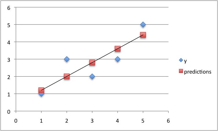
Finally, we can plot the predictions as a line and compare it to the original dataset.

Predictions For Small Contrived Dataset For Simple Linear Regression

5. Predict Insurance

We now know how to implement a simple linear regression model.

Let’s apply it to the Swedish insurance dataset.

This section assumes that you have downloaded the dataset to the file insurance.csv and it is available in the current working directory.

We will add some convenience functions to the simple linear regression from the previous steps.

Specifically a function to load the CSV file called load_csv(), a function to convert a loaded dataset to numbers called str_column_to_float(), a function to evaluate an algorithm using a train and test set called train_test_split() a function to calculate RMSE called rmse_metric() and a function to evaluate an algorithm called evaluate_algorithm().

The complete example is listed below.

A training dataset of 60% of the data is used to prepare the model and predictions are made on the remaining 40%.

# Simple Linear Regression on the Swedish Insurance Dataset
from random import seed
from random import randrange
from csv import reader
from math import sqrt

# Load a CSV file
def load_csv(filename):
	dataset = list()
	with open(filename, 'r') as file:
		csv_reader = reader(file)
		for row in csv_reader:
			if not row:
				continue
			dataset.append(row)
	return dataset

# Convert string column to float
def str_column_to_float(dataset, column):
	for row in dataset:
		row[column] = float(row[column].strip())

# Split a dataset into a train and test set
def train_test_split(dataset, split):
	train = list()
	train_size = split * len(dataset)
	dataset_copy = list(dataset)
	while len(train) < train_size:
		index = randrange(len(dataset_copy))
		train.append(dataset_copy.pop(index))
	return train, dataset_copy

# Evaluate an algorithm using a train/test split
def evaluate_algorithm(dataset, algorithm, split, *args):
	train, test = train_test_split(dataset, split)
	test_set = list()
	for row in test:
		row_copy = list(row)
		row_copy[-1] = None
		test_set.append(row_copy)
	predicted = algorithm(train, test_set, *args)
	actual = [row[-1] for row in test]
	rmse = rmse_metric(actual, predicted)
	return rmse

# Calculate the mean value of a list of numbers
def mean(values):
	return sum(values) / float(len(values))

# Calculate covariance between x and y
def covariance(x, mean_x, y, mean_y):
	covar = 0.0
	for i in range(len(x)):
		covar += (x[i] - mean_x) * (y[i] - mean_y)
	return covar

# Calculate the variance of a list of numbers
def variance(values, mean):
	return sum([(x-mean)**2 for x in values])

# Simple linear regression on insurance dataset
seed(1)
# load and prepare data
filename = 'insurance.csv'
dataset = load_csv(filename)
for i in range(len(dataset[0])):
	str_column_to_float(dataset, i)
# evaluate algorithm
split = 0.6
rmse = evaluate_algorithm(dataset, simple_linear_regression, split)
print('RMSE: %.3f' % (rmse))

# Simple Linear Regression on the Swedish Insurance Dataset

from random import seed

from random import randrange

from csv import reader

from math import sqrt

# Load a CSV file

def load_csv(filename):

dataset = list()

with open(filename, 'r') as file:

csv_reader = reader(file)

for row in csv_reader:

if not row:

continue

dataset.append(row)

return dataset

# Convert string column to float

def str_column_to_float(dataset, column):

for row in dataset:

row[column] = float(row[column].strip())

# Split a dataset into a train and test set

def train_test_split(dataset, split):

train = list()

train_size = split * len(dataset)

dataset_copy = list(dataset)

while len(train) < train_size:

index = randrange(len(dataset_copy))

train.append(dataset_copy.pop(index))

return train, dataset_copy

# Calculate root mean squared error

def rmse_metric(actual, predicted):

sum_error = 0.0

for i in range(len(actual)):

prediction_error = predicted[i] - actual[i]

sum_error += (prediction_error ** 2)

mean_error = sum_error / float(len(actual))

return sqrt(mean_error)

# Evaluate an algorithm using a train/test split

def evaluate_algorithm(dataset, algorithm, split, *args):

train, test = train_test_split(dataset, split)

test_set = list()

for row in test:

row_copy = list(row)

row_copy[-1] = None

test_set.append(row_copy)

predicted = algorithm(train, test_set, *args)

actual = [row[-1] for row in test]

rmse = rmse_metric(actual, predicted)

return rmse

# Calculate the mean value of a list of numbers

def mean(values):

return sum(values) / float(len(values))

# Calculate covariance between x and y

def covariance(x, mean_x, y, mean_y):

covar = 0.0

for i in range(len(x)):

covar += (x[i] - mean_x) * (y[i] - mean_y)

return covar

# Calculate the variance of a list of numbers

def variance(values, mean):

return sum([(x-mean)**2 for x in values])

# Calculate coefficients

def coefficients(dataset):

x = [row[0] for row in dataset]

y = [row[1] for row in dataset]

x_mean, y_mean = mean(x), mean(y)

b1 = covariance(x, x_mean, y, y_mean) / variance(x, x_mean)

b0 = y_mean - b1 * x_mean

return [b0, b1]

# Simple linear regression algorithm

def simple_linear_regression(train, test):

predictions = list()

b0, b1 = coefficients(train)

for row in test:

yhat = b0 + b1 * row[0]

predictions.append(yhat)

return predictions

# Simple linear regression on insurance dataset

seed(1)

# load and prepare data

filename = 'insurance.csv'

dataset = load_csv(filename)

for i in range(len(dataset[0])):

str_column_to_float(dataset, i)

# evaluate algorithm

split = 0.6

rmse = evaluate_algorithm(dataset, simple_linear_regression, split)

print('RMSE: %.3f' % (rmse))

Running the algorithm prints the RMSE for the trained model on the training dataset.

A score of about 33 (thousands of Kronor) was achieved, which is much better than the Zero Rule algorithm that achieves approximately 81 (thousands of Kronor) on the same problem.

1	RMSE: 33.630

Extensions

The best extension to this tutorial is to try out the algorithm on more problems.

Small datasets with just an input (x) and output (y) columns are popular for demonstration in statistical books and courses. Many of these datasets are available online.

Seek out some more small datasets and make predictions using simple linear regression.

Did you apply simple linear regression to another dataset?
Share your experiences in the comments below.

Review

In this tutorial, you discovered how to implement the simple linear regression algorithm from scratch in Python.

Specifically, you learned:

How to estimate statistics from a training dataset like mean, variance and covariance.
How to estimate model coefficients and use them to make predictions.
How to use simple linear regression to make predictions on a real dataset.

Do you have any questions?
Ask your question in the comments below and I will do my best to answer.

168 Responses to How To Implement Simple Linear Regression From Scratch With Python

Vineeth October 27, 2016 at 7:28 pm #

Hi Jason,

i have downloaded the csv file, but when i try to run the script against the file, i get the following error

” could not convert string to float: ‘X’ ”

this script stops at function def train_test_split(dataset, split)

can you confirm how your csv file is structured ?

Regards
Vineeth

Reply
- Jason Brownlee October 28, 2016 at 9:08 am #
  
  Sorry to hear that Vineeth.
  
  Totally my error, do not include the column headers in the small contrived dataset. Delete the first row.
  
  I will update the example.
  
  Reply
  - En-wai October 30, 2016 at 7:58 am #
    
    Hi Jason…..i have deleted the column headers X and Y along with all other descriptive info in the file but i kee getting this error:
    
    ” ValueError: could not convert string to float: i”
    
    here are the first 5 values in my csv file after removing the white space(replacing it with commas) and changing from european “,” to decimal “.”
    
    108,392.5
    19,46.2
    13,15.7
    124,422.2
    40,119.4
    
    Reply
    - Jason Brownlee October 30, 2016 at 8:59 am #
      
      Your file looks perfect.
      
      Confirm that you do not have any empty rows on the end of the file.
      
      Reply
    - ajay rana December 29, 2020 at 6:50 pm #
      
      what you should do , fetch column with as array
      
      x = np.array(data[[‘column’]] )
      
      fetch both column like this
      it will work
      
      Reply
  - Adeel December 3, 2021 at 12:54 am #
    
    Where I found csv file?
    
    Reply
    - Adrian Tam December 8, 2021 at 6:30 am #
      
      The link is in the post
      
      Reply
    - James Carmichael December 22, 2021 at 9:45 am #
      
      Hi Adeel…The data referenced can be found at the following link:
      
      https://college.cengage.com/mathematics/brase/understandable_statistics/7e/students/datasets/slr/frames/slr06.html
      
      When you arrive at this location, select the .xls file, download it and save it as a .csv file.
      
      Let me know if you need further clarification.
      
      Regards,
      
      Reply
Adrian Moldovan October 27, 2016 at 9:20 pm #

This is brilliant!
Thanks for talking the time to go through all the steps and explain literally… everything.

Reply
- Jason Brownlee October 28, 2016 at 9:09 am #
  
  You’re welcome Adrian, I’m glad you found it valuable.
  
  Reply
Nelson Silva October 28, 2016 at 2:11 am #

Hello Jason,
great tutorial!
It would be great if you also provided the code for the respective plots in python!
Especially the plot for the dataset 🙂

Thank you.

Reply
- Jason Brownlee October 28, 2016 at 9:16 am #
  
  Great suggestion Nelson, thanks.
  
  I was aiming to keep the use of libs to a minimum (e.g. no matplotlib or seaborn).
  
  Reply
- Rahul Sharma June 13, 2017 at 5:46 am #
  
  Hi Nelson, You can use pyplotlib library to create this kinf of scatter plot:
  
  Pls use this code to implement scatter plot:
  
  import pyplotlib.pyplot as py
  py.scatter(x_axis_value,y_axis_value,color=’black’)
  py.show()
  
  I hope this helps !
  
  Reply
venkat dabbara October 28, 2016 at 4:58 am #

predicted = algorithm(dataset, test_set)

where is algorithm defined???

Reply
- Jason Brownlee October 28, 2016 at 9:18 am #
  
  Great question Venkat.
  
  The “algorithm” argument in the evaluate_algorithm() function is a name of a function. We pass in the name of the function as “simple_linear_regression”. This means that when we execute algorithm() to make predictions in evaluate_algorithm(), we are in fact calling the simple_linear_regression() function.
  
  I did this to separate algorithm evaluation from algorithm implementation, so that the same test harness can be used for many different algorithms.
  
  Reply
En-wai October 28, 2016 at 9:14 pm #

under section 2. Calcuating covairiance i think the two meaning there is not quiet a clear. Pls check it.

“In fact, covariance is a generalization of correlation that is limited to two variables. Whereas covariance can be calculate between two or more variables.”???????

Reply
- Jason Brownlee October 29, 2016 at 7:42 am #
  
  Thanks En-wai, I have updated the language.
  
  I was trying to comment on how covariance is an abstraction of correlation to go from 2 groups of numbers to more than 2 groups of numbers.
  
  Reply
Ram October 29, 2016 at 1:06 am #

Hi,

I got clear idea on linear regression. Thank You.

We do calculate linear regression with SciPi library as below.

regr = linear_model.LinearRegression()

regr.fit(X_train, y_train).

Please clarify whether all this calculation will happen behind the scenes when we call the above code.

Reply
- Jason Brownlee October 29, 2016 at 9:25 am #
  
  Hi Ram,
  
  There are more efficient approaches to implement these algorithms using linear algebra. I expect this these more efficient approaches are being used behind the scenes.
  
  Implementing algorithms is great for learning how they work, but it is not a good idea to use these from scratch implementations in production.
  
  Reply
Aliyu A. Aziz October 29, 2016 at 6:03 pm #

Hi Jason,

Many thanks for this easy to follow LR from scratch. I have noticed Line 9

file = open(filename, “rb”)

is opening the file in text mode and causing the “Error: iterator should return strings, not bytes (did you open the file in text mode?)”

Changing ‘rb’ to ‘rt’ or ‘r’
file = open(filename, “rt”)

fixes the error.

Best regards

Reply
- Jason Brownlee October 30, 2016 at 8:54 am #
  
  Great, thanks Aliyu.
  
  It does work on my platform, but I will make the example more portable.
  
  Reply
saimadhu November 3, 2016 at 6:06 pm #

Hi,
Jason Brownlee

Thanks a lot for such an amazing post on simple linear regression. This post is the best tutorial to get the clear picture about simple linear regression analysis and I felt this post is the must read before learning the multi-regression analysis.

Reply
- Jason Brownlee November 4, 2016 at 9:06 am #
  
  Thanks saimadhu, I’m glad you found it useful.
  
  Reply
Johnny December 13, 2016 at 4:45 am #

Another great one and I love these foundation ones. Also, you get right into the steps/meat of it and you do not leave out cosmetics – just wrap those up neatly at the end. Thank you sir.

I would like to see/study this same type of process for datasets pertaining to the basic types of business. Specifically, how to produce good dataset and properly frame up problem areas, for business. Do you recommend any books?

Reply
- Jason Brownlee December 13, 2016 at 8:09 am #
  
  Thanks Johnny.
  
  Sorry, I don’t know of good books like that. It is an empirical pursuit – more of a craft. The best education is practice.
  
  Reply
Aslam March 12, 2017 at 4:39 am #

I am a beginner and found this very useful.

Thank you sir !

Reply
- Jason Brownlee March 12, 2017 at 8:28 am #
  
  I’m glad to hear it!
  
  Reply
Girish March 25, 2017 at 2:58 am #

How go we plot the graph using code

Reply
- Jason Brownlee March 25, 2017 at 7:39 am #
  
  You can use matplotlib:
  
  from matplotlib import pyplot pyplot.plot(x, y) pyplot.show()
  
  1
  2
  3
  
  from matplotlib import pyplot
  pyplot.plot(x, y)
  pyplot.show()
  
  Reply
  - Tamil January 3, 2019 at 1:27 am #
    
    I tried this but it gives empty graph.
    
    Reply
Nemanja April 2, 2017 at 5:33 am #

Hy, how can we plot a line of regression on our graph? And what we can do to reduce a rmse?Thanks

Reply
- Jason Brownlee April 2, 2017 at 6:33 am #
  
  You can evaluate the RMSE each epoch/iteration, save the RMSE values in an array and plot the array using matplotlib.
  
  Reply
Sean April 3, 2017 at 4:36 am #

what is the relationship between numpy.cov() , numpy.var() methods and your covariance() , variance() calculations ? I get very different results between the two.

Thanks

Reply
- Daniel L April 27, 2018 at 12:08 pm #
  
  Covariance and variance both should be divided by ‘n’ (for some reason he does not do it) , but it looses it’s significance for evaluate b1 [ b1= cov/var ].
  
  Reply
  - Aiden April 10, 2020 at 5:59 am #
    
    still bad practice…would you agree Jason?
    
    Reply
    - Mahaprasad June 19, 2023 at 6:07 pm #
      
      Hey Jason, could you please verify this?
      
      Shouldn’t the variance be divided by N in the formula?
      
      How can the variance of this data: [1,2,3,4,5] be 10?
      It doesn’t make sense.
      
      Reply
      - James Carmichael June 20, 2023 at 9:55 am #
        
        Hi Mahaprasad…The following resource may help add clarity:
        
        https://www.wikihow.com/Calculate-Variance
Abhishek April 28, 2017 at 3:25 pm #

Its a great article thankyou for helping us…

Reply
- Jason Brownlee April 29, 2017 at 7:21 am #
  
  Thanks Abhishek, I’m glad that you found it useful.
  
  Reply
Nuwan C May 4, 2017 at 1:30 pm #

Hi Jason,
Thank you for another great tutorial.
What does the Zero Based algorithm do and why it use in her?

Thank you

Reply
- Jason Brownlee May 5, 2017 at 7:28 am #
  
  Do you mean the Zero Rule algorithm?
  
  See this post for a description and worked example:
  https://machinelearningmastery.mystagingwebsite.com/implement-baseline-machine-learning-algorithms-scratch-python/
  
  Reply
John David Kromkowski May 5, 2017 at 2:28 am #

Nice work

Maybe tiny typo:

covariance = sum((x(i) – mean(x)) * (y – mean(y)))

should be

covariance = sum((x(i) – mean(x)) * (y(i) – mean(y)))

You have it correct in the actual code

Reply
- Jason Brownlee May 5, 2017 at 7:32 am #
  
  Thanks John. Fixed.
  
  Reply
Etienne May 20, 2017 at 6:35 pm #

Good day Jason

My model is y = b0 + (b1 * x) – (b2 / (b3+x)), which gives an asymptotic approach in a flocculation process. While I get a good data fit using the scipy curve_fit routine, I do not know how to get the leverage, the diagonal elements of the hat matrix H. Whereas in your model, the X system matrix would be formulated as:

^y = H.y

and H is X(XT.X)**-1.XT, where XT is the transpose of X

In your model X.^b would be:

[ 1 x0 ] [b0]
[ 1 x1 ] [b1]
[ 1 x2 ] .
[ 1 x3 ]
[ .. .. ]

But what would it be in my case?

Another problem is how to solve for H, so I can get the diagonal elements hii.

Any help would be greatly appreciated.

Reply
suguna May 24, 2017 at 4:45 am #

I removed columns header from csv file(Insurance CSV)

then Iam getting this following error:

ValueError: could not convert string to float: female

Reply
- Rahul Sharma June 13, 2017 at 5:47 am #
  
  suguna , you need to remove all the empty cells in your csv, if any are present. That is what is causing this error
  
  Reply
Rahul Sharma June 14, 2017 at 2:21 am #

Hi Jason,

As per the derivation : https://en.wikipedia.org/wiki/Standard_deviation

Variance = Avg (xi – xMean)^2

But here in algorithm you have used it as : sum([(x-mean)**2 for x in values])

which is not average but only some of squared difference. Is this some kind of modification?

Reply
- Rahul Sharma June 15, 2017 at 10:12 pm #
  
  Hi Jason. Can you please clarify this doubt.
  
  Reply
Digvijay Rana June 15, 2017 at 5:10 am #

Thankyou very much Sir,
I had been looking for someplace to start implenting algos myself. This is best tutorial i have read by far. Waiting fo other algorithm’s simple implementations.

Reply
- Jason Brownlee June 15, 2017 at 8:53 am #
  
  Thanks, I’m glad to hear that.
  
  I have many right here:
  https://machinelearningmastery.mystagingwebsite.com/machine-learning-algorithms-from-scratch/
  
  Reply
- noname June 24, 2017 at 3:13 pm #
  
  too late to board the ML bus ..Digvijay..
  
  Reply
  - Jason Brownlee June 25, 2017 at 5:58 am #
    
    Never too late.
    
    Reply
Vaibhav June 17, 2017 at 11:08 pm #

Thanks a lot sir ! . Its a best description so far .

Reply
- Jason Brownlee June 18, 2017 at 6:31 am #
  
  I’m glad to hear it.
  
  Reply
Kris July 6, 2017 at 11:20 pm #

I’m confused about your definition of covariance. Generally it’s finally divided by (n – 1) where n is the number of samples, where as there is no such operation carried out through out the code. Can you please clarify ?

Reply

Soumik Rakshit July 13, 2017 at 1:45 am #

I am unable to download the dataset as a csv file. Can someone please help me???

Jason Brownlee July 13, 2017 at 9:57 am #

Here is the raw file:

Auto Insurance in Sweden

In the following data

X = number of claims

Y = total payment for all the claims in thousands of Swedish Kronor

for geographical zones in Sweden

Reference: Swedish Committee on Analysis of Risk Premium in Motor Insurance

http://college.hmco.com/mathematics/brase/understandable_statistics/7e/students/datasets/

slr/frames/frame.html

X Y

108 392,5

19 46,2

13 15,7

124 422,2

40 119,4

57 170,9

23 56,9

14 77,5

45 214

10 65,3

5 20,9

48 248,1

11 23,5

23 39,6

7 48,8

2 6,6

24 134,9

6 50,9

3 4,4

23 113

6 14,8

9 48,7

9 52,1

3 13,2

29 103,9

7 77,5

4 11,8

20 98,1

7 27,9

4 38,1

0 0

25 69,2

6 14,6

5 40,3

22 161,5

11 57,2

61 217,6

12 58,1

4 12,6

16 59,6

13 89,9

60 202,4

41 181,3

37 152,8

55 162,8

41 73,4

11 21,3

27 92,6

8 76,1

3 39,9

17 142,1

13 93

13 31,9

15 32,1

8 55,6

29 133,3

30 194,5

24 137,9

9 87,4

31 209,8

14 95,5

53 244,6

26 187,5

You will need to convert the “,” to “.” and replace the space between columns with “,”.

uma maheswari July 16, 2017 at 9:09 pm #

hi jason

can you tell how do we implement the linear regression on image dataset

Reply
- Jason Brownlee July 17, 2017 at 8:46 am #
  
  Perhaps linear regression is a bad fit image data.
  
  Convolutional neural networks are very popular for image data:
  https://machinelearningmastery.mystagingwebsite.com/crash-course-convolutional-neural-networks/
  
  Reply
Pierce Ng July 31, 2017 at 1:39 am #

Hi Jason,

Great stuff! Thanks for the exposition.

I implemented a no-shuffling version of train_test_split which always takes the first 38 entries as training data and the last 25 entries as test data. The program gives RMSE of 45.23.

Your RMSE of 38.339 is from the randomization in train_test_split with seed(1). If I try with seed(2) then the RMSE is 37.734.

What’s the next step with different values of RMSE?

Reply
- Jason Brownlee July 31, 2017 at 8:16 am #
  
  This is the variance of the method.
  
  Ideally, we would evaluate the algorithm multiple times and report the mean and standard deviation of the model.
  
  Does that help?
  
  Reply
  - Pierce Ng August 6, 2017 at 3:20 pm #
    
    It does, thanks.
    
    I ported your Python code to Pharo Smalltalk and wrote a blog post. See http://www.samadhiweb.com/blog/2017.08.06.dataframe.html.
    
    Reply
    - Jason Brownlee August 7, 2017 at 8:39 am #
      
      Very cool Pierce. Nice work!
      
      I used to work with a dev who was a massive small talk fan.
      
      Reply
Eoin Kenny August 11, 2017 at 3:14 am #

That is NOT the formula for variance… you’re supposed to divide by n or n-1, what is going on?

Reply
- Jason Brownlee August 11, 2017 at 6:43 am #
  
  Might be population vs sample variance.
  
  Reply
Tanmay September 1, 2017 at 2:42 am #

Hi Jason, why this *args parameter in the evaluate_algorithm function?

Reply
- Jason Brownlee September 1, 2017 at 6:49 am #
  
  So we can provide a variable number parameters for the algorithm to the evaluat_algorithm() function.
  
  It is generic for different algorithms.
  
  Reply
vedang September 15, 2017 at 2:19 am #

How do we predict the value of y, given x. Also how obtain the accuracy?

Reply
- Jason Brownlee September 15, 2017 at 12:16 pm #
  
  This is all of applied machine learning.
  
  Perhaps you might be best starting with Weka:
  https://machinelearningmastery.mystagingwebsite.com/start-here/#weka
  
  Reply
Barrys September 15, 2017 at 1:27 pm #

Hi Jason,

Thanks for your great articles. They are very helpful to me.

Something is not clear to me. Why we calculated RMSE and what it means exactly? I was expecting you would calculate the accuracy of predictions from the test data as you did in your KNN post.

Thanks.

Reply
- Jason Brownlee September 16, 2017 at 8:36 am #
  
  RMSE is root mean squared error and is the error of the predictions in the same units as the output variable.
  
  You cannot calculate accuracy for a regression problem. Accuracy refers to the percentage of correct label predictions out of all label predictions made. We do not predict a label in regression, we predict a quantity.
  
  Reply
  - Barrys September 16, 2017 at 1:28 pm #
    
    So we need to run another algorithm to predict its label? How can I use y value for a given x without knowing its label (that’s linear regression as i understood)? What kind of problems does the linear regression solve?
    
    It would be better to explain RMSE in the document and why we calculate it? it is mentioned but not explained.
    
    Reply
    - Jason Brownlee September 17, 2017 at 5:25 am #
      
      Linear regression is for problems where we want to predict a quantity, called regression problems.
      
      If you have a dataset where you need to predict a label, you cannot use linear regression. You will need another algorithm like logistic regression.
      
      Reply
Rizvi October 11, 2017 at 9:23 pm #

Hi Jason,

This is an awesome post for beginners.

Currently, we are fitting a polynomial with 2 coefficients to the data. If we extend this approach to higher order polynomial, will that come under the scope of non-linear regression? Also, will increasing the polynomial order improve the estimation accuracy?

Reply
- Jason Brownlee October 12, 2017 at 5:28 am #
  
  It may improve accuracy, or it may over fit the data. Try it and see.
  
  Use a robust test harness to ensure you do not trick yourself.
  
  Reply
Melina October 17, 2017 at 12:08 am #

Great tutorial! Thank you 🙂

I am preparing a demo for simple linear regression and I plan to show the code using sklearn and compare it to “own” regression algorithm code, tweaked version of yours!

I am stuck at one thing in your code and that is the variance formula/equation.
* You are using: Variance = Sum( (x – mean(x))^2 )
* Should it not be: Variance = Sum( (x – mean(x))^2 ) / N

I am probably just confused so please correct me to the right thinking if I am.

Reply
- Jason Brownlee October 17, 2017 at 5:49 am #
  
  It is not normalized. See here for more information:
  https://en.wikipedia.org/wiki/Simple_linear_regression
  
  Reply
Adilah December 6, 2017 at 12:46 am #

Hi Jason, can this method be used to predict the consumption of a type of product by customer? (sorry for my english )

Reply
- Jason Brownlee December 6, 2017 at 9:04 am #
  
  I would recommend this process to work through your problem systematically:
  https://machinelearningmastery.mystagingwebsite.com/start-here/#process
  
  Reply
Ronnie Mukherjee December 16, 2017 at 10:01 pm #

Does anyone have the RMSE using the entire swedish insurance dataset for both training and testing (for verification)?

Thanks

Reply
Himsikha hazarika January 10, 2018 at 8:55 pm #

The dataset was already in float format.so,i commented out :

# Convert string column to float
”’def str_column_to_float(dataset, column):
for row in dataset:
row[column] = float(row[column].strip())”’
_______________________
X Y
108 392.5
19 46.2
13 15.7
124 422.2
40 119.4
;;;;;;_
______________________________

but the i got the below error:

Traceback (most recent call last):
File “linear.py”, line 97, in
rmse = evaluate_algorithm(dataset, simple_linear_regression, split)
File “linear.py”, line 50, in evaluate_algorithm
predicted = algorithm(train, test_set, *args)
File “linear.py”, line 82, in simple_linear_regression
b0, b1 = coefficients(train)
File “linear.py”, line 74, in coefficients
x_mean, y_mean = mean(x), mean(y)
File “linear.py”, line 57, in mean
return sum(values) / float(len(values))
TypeError: unsupported operand type(s) for +: ‘int’ and ‘str’

Reply
- Jason Brownlee January 11, 2018 at 5:49 am #
  
  Sorry, I don’t know the cause of your error.
  
  Reply
  - Gosia March 15, 2019 at 1:49 am #
    
    you need to convert the dataframe to a list
    
    Reply
Faraz January 22, 2018 at 2:20 am #

Can anyone help me that how to convert the “,” to “.” and replace the space between columns with “,” ? It would be great if you upload the code!

Reply
- Jason Brownlee January 22, 2018 at 4:46 am #
  
  Sorry, perhaps a course on basic programming would be a good place to start.
  
  Reply
- Shashank April 23, 2018 at 8:09 pm #
  
  Use linux 🙂 Sed command will help you out in one go 😀
  
  Reply
Shashank April 23, 2018 at 8:08 pm #

HI Jason, Could you pls help me with algorithm() function in line 50 of the code ? It is not defined anywhere …… ? Is it some pre-defined function … I think it is simple_linear_regression() function only as replacing it with the latter, I get same results 🙂 Pls assist.

Reply
- Jason Brownlee April 24, 2018 at 6:33 am #
  
  It is a reference to a function that we pass in as an argument. Specifically it is executing simple_linear_regression()
  
  If you are new to python programming, perhaps start here:
  https://machinelearningmastery.mystagingwebsite.com/faq/single-faq/how-do-i-get-started-with-python-programming
  
  Reply
Aarabhi Putty April 27, 2018 at 6:38 pm #

Thank you so much Jason. It is very useful and understandable.

Reply
- Jason Brownlee April 28, 2018 at 5:26 am #
  
  I’m glad it helped.
  
  Reply
ranjan May 3, 2018 at 7:06 pm #

Hi Jason,

thanks for the code and making it easy to understand. I edited the code and selected half values starting from the end as training set and got an RMSE of 35.365.

whereas I see your code will select 60% of the values as training set arbitrarily and gives the RMSE output as 38.339.

Q: what should be the correct approach between the both?

Reply
- Jason Brownlee May 4, 2018 at 7:39 am #
  
  It is a contrived example, we can make it up.
  
  Generally, the choice of training and test dataset is dependent on the type of problem and what is known about the data.
  
  This might give you some ideas:
  https://machinelearningmastery.mystagingwebsite.com/faq/single-faq/how-do-i-evaluate-a-machine-learning-algorithm
  
  Reply
Balghari May 8, 2018 at 6:05 am #

How to find the beta_0 and beta values in multiple linear regression?plz guide me

Reply
- Jason Brownlee May 8, 2018 at 6:18 am #
  
  Via an optimisation procedure, such as the method used in the linear algebra formulation or gradient descent.
  
  Reply
manohar May 14, 2018 at 3:02 pm #

How you get RMSE 72.251 using Zero Rule algorithm for insurance dataset

im using your below post

https://machinelearningmastery.mystagingwebsite.com/implement-baseline-machine-learning-algorithms-scratch-python/

This is a Regression problem, so im using Regression Zero Rule algorithm
for your post i didn’t get

for eg:

108,392.5
19,46.2
13,15.7
124,422.2
40,119.4

this is a insurance dataset how you get RMSE 72.251 using Zero Rule algorithm
can you try to figure out please ?

Reply
- Jason Brownlee May 15, 2018 at 7:50 am #
  
  What problem are you having exactly?
  
  Reply
manohar palanisamy May 15, 2018 at 6:38 pm #

Actually i don’t know how you get RMSE 72.251 using Zero Rule algorithm for first five observations

108+19+13+124+40=304

mean=304/5=60.8

i’m getting 60.8 as per your below link you mention in the regression section

https://machinelearningmastery.mystagingwebsite.com/implement-baseline-machine-learning-algorithms-scratch-python/

Reply
- Jason Brownlee May 16, 2018 at 6:00 am #
  
  Zero Rule will calculate the average of all values in the training dataset in order to make a prediction on the test dataset.
  
  Reply
manohar palanisamy May 15, 2018 at 6:39 pm #

please let me tell ?

Reply
Harshit Jain June 9, 2018 at 8:44 pm #

Are gradient descent and analytic approach not implemented in real world?

Reply
- Jason Brownlee June 10, 2018 at 6:03 am #
  
  The linear algebra approach is how most libraries solve the linear regression equation, but they require all data to be in memory and to confirm to the expectations of the method (Gaussian, uncorrelated variates, etc.)
  
  Reply
Gourav Singh Bais June 15, 2018 at 2:55 pm #

How can I draw the scatter plot of x and y long with all the predictions ?

Reply
- Jason Brownlee June 16, 2018 at 7:23 am #
  
  You can use the scatter() function from matplotlib.
  
  Reply
Boris July 3, 2018 at 10:51 pm #

Hi Jason
I’m newbie in ML. Great example and tutorial. Please advise how code should look like if there is more than one column for X part? for example there are 6 columns? Thanks

Reply
- Jason Brownlee July 4, 2018 at 8:23 am #
  
  You can modify the code to support multiple inputs or use a library like sklearn.
  
  Reply
Betaman July 12, 2018 at 12:44 am #

I don’t understand the gravity of the code
Could it be sent a one code altogether

Great post though

Reply
- Jason Brownlee July 12, 2018 at 6:26 am #
  
  If this tutorial is not a good fit for you, please try a google search for another?
  
  Reply
Prajna p n July 12, 2018 at 4:57 pm #

As per the variance formula you have provided in the article :
variance = sum( (x – mean(x))^2 ) ..But ideally as per the formula it is variance = sum( (x – mean(x))^2 )/(n-1).

Reply
Aditi August 12, 2018 at 10:59 pm #

Hello Jason,

I tried the program . It gives me the below error . Would you be able to tell me what’s wrong happening here ?

ipython-input-4-eae09e62a94d> in load_csv(filename)
6 if not row:
7 continue
—-> 8 dataset.append()
9 return dataset
10

TypeError: append() takes exactly one argument (0 given)

Reply
- Jason Brownlee August 13, 2018 at 6:17 am #
  
  Perhaps confirm you are using Python 2.7?
  
  Reply
  - mrunal August 22, 2018 at 4:40 pm #
    
    This is a great tutorial. I loved it. My regression analysis has been solved using your tutorial. Moreover, I have 6 input and 6 output of 4000 datasets. can you provide me neural network fitting code in python??
    
    Reply
    - Jason Brownlee August 23, 2018 at 6:12 am #
      
      Well done.
      
      Yes, you can have a vector output. I recommend using Keras:
      https://machinelearningmastery.mystagingwebsite.com/start-here/#deeplearning
      
      Reply
Narender August 23, 2018 at 3:03 am #

Wonderful website and golden resource. Thanks Jason!

Reply
- Jason Brownlee August 23, 2018 at 6:15 am #
  
  Thanks, I hope it helps.
  
  Reply
Syed Fakhar Alam September 3, 2018 at 11:42 pm #

Hi jason, how can I implement svm model in python using tensorflow.

Reply
- Jason Brownlee September 4, 2018 at 6:07 am #
  
  Sorry, I don’t have any tutorials on tensorflow.
  
  I would recommend using sklearn to implement an SVM model:
  https://machinelearningmastery.mystagingwebsite.com/start-here/#python
  
  Reply
Karthik Kolle February 17, 2019 at 2:21 am #

Hi
Im a beginner in Machine Learning.

This might sound like a stupid question, but I want to ask it anyway.

What exactly does the final value printed on the screen signify?

Also, if I were to include plotting, how do I go ahead with that?

Reply
- Jason Brownlee February 17, 2019 at 6:35 am #
  
  In the example, we learned how to predict an output given an input for a small contrived problem.
  
  You can create a plot in excel as I did and show the raw relationship between inputs and outputs and the relationship between inputs and predictions.
  
  Reply
Suchha March 29, 2019 at 5:48 pm #

Hi Jason,

This is an awesome post.. My search for regression code ended here..
I highly appreciate your patience.. You have addressed each and every comment till date…
Kudos to you.. May god bless you…

Reply
- Jason Brownlee March 30, 2019 at 6:24 am #
  
  Happy to help.
  
  Reply
Laxmikant May 28, 2019 at 9:31 pm #

Just a suggestion, You could have prepared a video instead, which might have included all the answers at the same time. 🙂 it’d have saved our time reading your valuable blogs 😛

BTW, I found your posts very informative,wonderful articles for beginners. Thanks very much 🙂

Reply
- Jason Brownlee May 29, 2019 at 8:42 am #
  
  Thanks for the suggestion.
  
  I find video a poor medium for teaching. Way too passive.
  
  We learn by doing in applied ML. Which includes reading, writing, coding, experimenting, etc.
  
  Reply
Red August 11, 2019 at 10:43 pm #

Thanks a lot Jason,
Your post very informative and helpful.Do you have a similar post on Huber Regression ??

Reply
- Jason Brownlee August 12, 2019 at 6:37 am #
  
  Thanks.
  
  Not at this stage, thanks for the suggestion!
  
  Reply
v.c September 25, 2019 at 4:31 am #

Hi Jason,

Thanks for your wonderful blog, referring your blog I’ve implemented same in C. It can be found at – https://github.com/novice-programmer/numerical-programing/tree/master/simple_linear_regression . Please share your suggestions if any.

Reply
- Jason Brownlee September 25, 2019 at 6:04 am #
  
  Well done!
  
  Reply
Shoumitra Bala October 19, 2019 at 10:18 am #

Really helpful and good content to kick off ML for beginners

Reply
- Jason Brownlee October 20, 2019 at 6:14 am #
  
  Thanks!
  
  Reply
lavanya October 21, 2019 at 9:03 pm #

Hi jason,

Its really use full..

Can you help us assumptions of a linear regression and what are the ways to achieve those assumptions like normal distribution of error, equal variance, independence

Thanks in advance

Reply
- Jason Brownlee October 22, 2019 at 5:47 am #
  
  I believe wiki has a good list of assumptions for linear regression
  https://en.wikipedia.org/wiki/Linear_regression#Assumptions
  
  Reply
Ashish November 15, 2019 at 7:30 am #

Hi Jason,

May you please me with the following doubts.

1) how this complete process is different from Sklearn LinearRegression()?

2) how could we be sure that we get the best optimum line to fit our model i.e. our model ‘s cost is minimized to the extent it is possible. Like we get at MLE and gradient descent.

3) Is this method best suited for the large datasets?

Thanks

Ashish Arora

Reply
- Jason Brownlee November 15, 2019 at 7:58 am #
  
  Sklearn will use an analytical solution, e.g. linalg.
  
  Minimizing MSE will achieve an “optimal” fit of the model, it may or may not be the best model for the dataset.
  
  This method is only suited for two variables (one in, one out) and when the relevant coefficients can be calculated or estimated.
  
  Reply
chase December 10, 2019 at 10:35 am #

HI Jason, if I just wanted to test the linear regression function without the rmse how would I do so? thanks

Reply
- Jason Brownlee December 10, 2019 at 1:36 pm #
  
  What do you mean exactly?
  
  Reply
  - Chase December 10, 2019 at 1:53 pm #
    
    How could I test the simple_linear_regression function without the “evaluate_algorithm” and “rmse_metric” function? Or is that not possible?
    
    Reply
    - Jason Brownlee December 11, 2019 at 6:46 am #
      
      Yes, you can train the coefficients and use them directly to make a prediction.
      
      Reply
Abhishek Panchal December 26, 2019 at 10:51 pm #

I getting this error while trying to run the code:
—————————————————————————
ValueError Traceback (most recent call last)
in
1 split = 0.6
—-> 2 rmse = evaluate_algorithm(dataset, simple_linear_regression, split)

in evaluate_algorithm(dataset, algorithm, split, *args)
1 def evaluate_algorithm(dataset, algorithm, split, *args):
—-> 2 train, test = train_test_split(dataset, split)
3 test_set = list()
4 for row in test:
5 row_copy = list(row)

in train_test_split(dataset, split)
4 dataset_copy = list(dataset)
5 while len(train) 6 index = randrange(len(dataset_copy))
7 train.append(dataset_copy.pop(index))
8 return train, dataset_copy

~\Anaconda3\lib\random.py in randrange(self, start, stop, step, _int)
188 if istart > 0:
189 return self._randbelow(istart)
–> 190 raise ValueError(“empty range for randrange()”)
191
192 # stop argument supplied.

ValueError: empty range for randrange()

Any Idea why isn’t it’s working?

Reply
- Jason Brownlee December 27, 2019 at 6:34 am #
  
  Sorry to hear that, I have some suggestions here:
  https://machinelearningmastery.mystagingwebsite.com/faq/single-faq/why-does-the-code-in-the-tutorial-not-work-for-me
  
  Reply
DM March 28, 2020 at 9:24 am #

Isn’t it an error that the output array of predicted points is
1.1999999999999995,
1.9999999999999996,
3.5999999999999996,
2.8,
4.3999999999999995

It seems that 3 and 4 elements are mixed up.

Reply
- Jason Brownlee March 29, 2020 at 5:48 am #
  
  How so?
  
  Reply
Siddharth Singh June 3, 2020 at 11:25 pm #

Hi Jason,
Help me in understanding
row_copy[-1] = None and
actual = [row[-1] for row in dataset]
from function evaluate_algorithm()

Reply
- Jason Brownlee June 4, 2020 at 6:23 am #
  
  The first sets the last value in the list to None, e.g. the output value so we cannot cheat.
  
  The second retrieves the last value for each row in the dataset, e.g. creates a list of just the predictions.
  
  Reply
Siddharth Singh June 5, 2020 at 2:51 am #

Thank You, Jason

Reply
- Jason Brownlee June 5, 2020 at 8:17 am #
  
  You’re welcome.
  
  Reply
Oleg June 19, 2020 at 9:03 am #

Thank you Jason! This is an amazing example.
Just to clarify, here we trained algorithm, then tested it.
So if I have a list of only “X” values, how can I pass them to a function to get output “Y” values? Let’s say I have 200 claims and I need a total payment for it?
Thank you

Reply
- Jason Brownlee June 19, 2020 at 1:11 pm #
  
  You can see an example of making a prediction in the final example, e.g with a row of data use:
  
  yhat = b0 + b1 * row[0]
  
  1
  
  yhat = b0 + b1 * row[0]
  
  Reply
Gideon Aswani September 2, 2020 at 9:38 pm #

Hi Jason

Thanks for sharing. This is a wonderful tutorial. I was able to follow and implement it in a Jupyter Notebook without any problems at all. I will be trying different datasets with appropriate changes to the code. Once more thank you.

Reply
- Jason Brownlee September 3, 2020 at 6:06 am #
  
  You’re welcome, well done!
  
  Reply
Santosh Khanal September 7, 2020 at 4:51 pm #

C:\Users\99193942\AppLockerExceptions\PycharmProject\Simple_linear_regression\venv\Scripts\python.exe C:/Users/99193942/AppLockerExceptions/PycharmProject/Simple_linear_regression/Predict_insurance.py
Traceback (most recent call last):
File “C:/Users/99193942/AppLockerExceptions/PycharmProject/Simple_linear_regression/Predict_insurance.py”, line 98, in
rmse = evaluate_algorithm(dataset, simple_linear_regression, split)
File “C:/Users/99193942/AppLockerExceptions/PycharmProject/Simple_linear_regression/Predict_insurance.py”, line 50, in evaluate_algorithm
predicted = algorithm(train, test_set, *args)
File “C:/Users/99193942/AppLockerExceptions/PycharmProject/Simple_linear_regression/Predict_insurance.py”, line 83, in simple_linear_regression
for row in test:
NameError: name ‘test’ is not defined

Reply
- Jason Brownlee September 8, 2020 at 6:47 am #
  
  Sorry to hear that you’re having trouble, these tips may help:
  https://machinelearningmastery.mystagingwebsite.com/faq/single-faq/why-does-the-code-in-the-tutorial-not-work-for-me
  
  Reply
  - Robin November 14, 2020 at 10:09 pm #
    
    Hi Jason,
    
    I just started deep learning Master’s I am doing a model to detect any malicious in modbus protocol which is used in industrial fields, do you have something to start with, your advice please
    
    Reply
    - Jason Brownlee November 15, 2020 at 6:25 am #
      
      Perhaps this process will help you work through your project:
      https://machinelearningmastery.mystagingwebsite.com/start-here/#process
      
      Reply
Fahmi December 2, 2020 at 12:47 pm #

Hi, Jason..
How do we can plot a graph from the result predictions of simple linear regession on the insurance dataset above by using code?
Thanks a lot

Reply
- Jason Brownlee December 2, 2020 at 1:20 pm #
  
  This tutorial gives an example of plotting the line for a regression model:
  https://machinelearningmastery.mystagingwebsite.com/robust-regression-for-machine-learning-in-python/
  
  Reply
Trupt September 2, 2021 at 7:28 pm #

Hi, Jason

master piece.

i just want to know that how do you get these starting values of B0 and B1

B1 = sum((x(i) – mean(x)) * (y(i) – mean(y))) / sum( (x(i) – mean(x))^2 )
B0 = mean(y) – B1 * mean(x)

, I am curious…

Reply
- Jason Brownlee September 3, 2021 at 5:30 am #
  
  Thanks!
  
  Arbitary. In practice, start with zero or a small random number.
  
  Reply
Sobia murtaza September 27, 2021 at 3:50 pm #

Using this code can i get linear regression to find cost funtion of any dataset?? Should i follow thes all step to finde cost function ??

Reply
- Adrian Tam September 28, 2021 at 9:32 am #
  
  Usually cost function is something you decided before doing regression. For example, linear regression for y=f(X) is to use mean squared error as cost.
  
  Reply
alifiya October 18, 2021 at 10:13 am #

I am getting an RMSE of 104 is it even possible (cause the value is supposed to be 0~1) what could be the reason

Reply
- Adrian Tam October 20, 2021 at 9:16 am #
  
  Possible. But that means your model is really bad. Think in this way, the range of your output y is 0 to 1, hence the standard deviation should not be bigger than 1. You are making error of 100 times the standard deviation.
  
  Reply
Alina March 24, 2022 at 12:47 pm #

Hello,
When I run my code it is giving me an error of float object is not subscriptable. The error is occurring in the coefficients function when trying to get the coefficients of the data. Do you know a solution for this

Reply
- James Carmichael March 25, 2022 at 1:51 pm #
  
  Hi Alina…Thanks for asking.
  
  I’m eager to help, but I just don’t have the capacity to debug code for you.
  
  I am happy to make some suggestions:
  
  Consider aggressively cutting the code back to the minimum required. This will help you isolate the problem and focus on it.
  Consider cutting the problem back to just one or a few simple examples.
  Consider finding other similar code examples that do work and slowly modify them to meet your needs. This might expose your misstep.
  Consider posting your question and code to StackOverflow.
  
  Reply
Burhan Bilen April 22, 2022 at 6:44 pm #

Hello Jason, thanks for the explanations and coding. I wonder that why some people use gradient descent to optimize cost and some other do not (in my case I did not use either, just used basic formulas). Is there any difference between?

Reply
- James Carmichael April 24, 2022 at 3:35 am #
  
  Hi Burhan…There are many optimization methods to select from. The following may be of interest:
  
  https://machinelearningmastery.mystagingwebsite.com/a-gentle-introduction-to-optimization-mathematical-programming/
  
  Reply
ankit February 22, 2023 at 1:52 am #

hey thanks for the wonderful blog, do you have any blog to implement same thing for polynomial regression,actually i have 5 candidate polynomial regression models which i have to estimate the parameters for

Reply
- James Carmichael February 22, 2023 at 8:23 am #
  
  Hi ankit…The following resource may be of interest:
  
  https://medium.com/analytics-vidhya/understanding-polynomial-regression-5ac25b970e18
  
  Reply
Vinícius Jean Ferreira August 1, 2023 at 12:10 am #

Hi, James.
Nice post! I am just struggling to understand: Linear Regression is really simple as that or there are more iterations on the algorithm to search for the best coefficients? I mean… it should use the Gradient Descent function to evaluate the error and minimize it, or am I wrong?

Thank you?

Reply
- James Carmichael August 1, 2023 at 9:10 am #
  
  Hi Vincius…Yes, gradient descent can be used as follows:
  
  https://machinelearningmastery.mystagingwebsite.com/a-gentle-introduction-to-gradient-descent-procedure/
  
  Reply

Navigation

How To Implement Simple Linear Regression From Scratch With Python

Description

Simple Linear Regression

Swedish Insurance Dataset

Tutorial

1. Calculate Mean and Variance

2. Calculate Covariance

3. Estimate Coefficients

4. Make Predictions

5. Predict Insurance

Extensions

Review

Discover How to Code Algorithms From Scratch!

No Libraries, Just Python Code.

Finally, Pull Back the Curtain on
Machine Learning Algorithms

More On This Topic

168 Responses to How To Implement Simple Linear Regression From Scratch With Python

Leave a Reply Click here to cancel reply.

Navigation

Description

Simple Linear Regression

Swedish Insurance Dataset

Tutorial

1. Calculate Mean and Variance

2. Calculate Covariance

3. Estimate Coefficients

4. Make Predictions

5. Predict Insurance

Extensions

Review

Discover How to Code Algorithms From Scratch!

No Libraries, Just Python Code.

Finally, Pull Back the Curtain on Machine Learning Algorithms

More On This Topic

168 Responses to How To Implement Simple Linear Regression From Scratch With Python

Leave a Reply Click here to cancel reply.

Finally, Pull Back the Curtain on
Machine Learning Algorithms