Simple Linear Regression Tutorial for Machine Learning

Last Updated on August 12, 2019

Linear regression is a very simple method but has proven to be very useful for a large number of situations.

In this post, you will discover exactly how linear regression works step-by-step. After reading this post you will know:

• How to calculate a simple linear regression step-by-step.
• How to perform all of the calculations using a spreadsheet.
• How to make predictions on new data using your the model.
• A shortcut that greatly simplifies the calculation.

This tutorial was written for developers and does not assume any prior background in mathematics or statistics.

This tutorial was written with the intention that you will follow along in your own spreadsheet, which will help to make the concepts stick.

Kick-start your project with my new book Master Machine Learning Algorithms, including step-by-step tutorials and the Excel Spreadsheet files for all examples.

Let’s get started.

Update #1: Fixed a bug in the calculation of RMSE.

Simple Linear Regression Tutorial for Machine Learning
Photo by Catface27, some rights reserved.

Tutorial Data Set

The data set we are using is completely made up.

Below is the raw data.

The attribute x is the input variable and y is the output variable that we are trying to predict. If we got more data, we would only have x values and we would be interested in predicting y values.

Below is a simple scatter plot of x versus y.

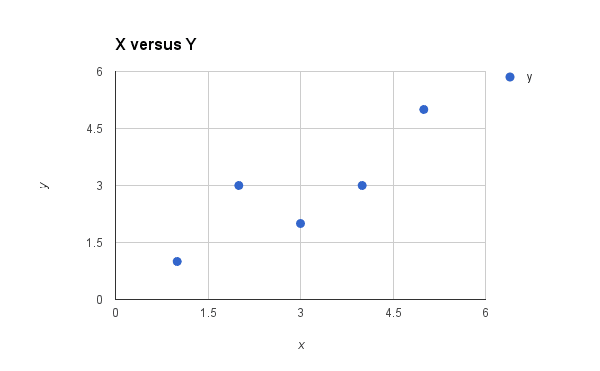
Plot of the Dataset for Simple Linear Regression

We can see the relationship between x and y looks kind of linear. As in, we could probably draw a line somewhere diagonally from the bottom left of the plot to the top right to generally describe the relationship between the data.

This is a good indication that using linear regression might be appropriate for this little dataset.

Get your FREE Algorithms Mind Map

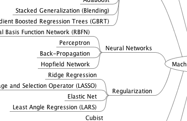
Sample of the handy machine learning algorithms mind map.

I've created a handy mind map of 60+ algorithms organized by type.

Download it, print it and use it. 

Simple Linear Regression

When we have a single input attribute (x) and we want to use linear regression, this is called simple linear regression.

If we had multiple input attributes (e.g. x1, x2, x3, etc.) This would be called multiple linear regression. The procedure for linear regression is different and simpler than that for multiple linear regression, so it is a good place to start.

In this section we are going to create a simple linear regression model from our training data, then make predictions for our training data to get an idea of how well the model learned the relationship in the data.

With simple linear regression we want to model our data as follows:

y = B0 + B1 * x

This is a line where y is the output variable we want to predict, x is the input variable we know and B0 and B1 are coefficients that we need to estimate that move the line around.

Technically, B0 is called the intercept because it determines where the line intercepts the y-axis. In machine learning we can call this the bias, because it is added to offset all predictions that we make. The B1 term is called the slope because it defines the slope of the line or how x translates into a y value before we add our bias.

The goal is to find the best estimates for the coefficients to minimize the errors in predicting y from x.

Simple regression is great, because rather than having to search for values by trial and error or calculate them analytically using more advanced linear algebra, we can estimate them directly from our data.

We can start off by estimating the value for B1 as:

B1 = sum((xi-mean(x)) * (yi-mean(y))) / sum((xi – mean(x))^2)

Where mean() is the average value for the variable in our dataset. The xi and yi refer to the fact that we need to repeat these calculations across all values in our dataset and i refers to the i’th value of x or y.

We can calculate B0 using B1 and some statistics from our dataset, as follows:

B0 = mean(y) – B1 * mean(x)

Not that bad right? We can calculate these right in our spreadsheet.

Estimating The Slope (B1)

Let’s start with the top part of the equation, the numerator.

First we need to calculate the mean value of x and y. The mean is calculated as:

1/n * sum(x)

Where n is the number of values (5 in this case). You can use the AVERAGE() function in your spreadsheet. Let’s calculate the mean value of our x and y variables:

mean(x) = 3

mean(y) = 2.8

Now we need to calculate the error of each variable from the mean. Let’s do this with x first:

Now let’s do that for the y variable

We now have the parts for calculating the numerator. All we need to do is multiple the error for each x with the error for each y and calculate the sum of these multiplications.

Summing the final column we have calculated our numerator as 8.

Now we need to calculate the bottom part of the equation for calculating B1, or the denominator. This is calculated as the sum of the squared differences of each x value from the mean.

We have already calculated the difference of each x value from the mean, all we need to do is square each value and calculate the sum.

Calculating the sum of these squared values gives us up denominator of 10

Now we can calculate the value of our slope.

B1 = 8 / 10

B1 = 0.8

Estimating The Intercept (B0)

This is much easier as we already know the values of all of the terms involved.

B0 = mean(y) – B1 * mean(x)

or

B0 = 2.8 – 0.8 * 3

or

B0 = 0.4

Easy.

Making Predictions

We now have the coefficients for our simple linear regression equation.

y = B0 + B1 * x

or

y = 0.4 + 0.8 * x

Let’s try out the model by making predictions for our training data.

We can plot these predictions as a line with our data. This gives us a visual idea of how well the line models our data.

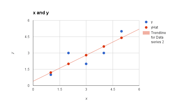
Simple Linear Regression Model

Estimating Error

We can calculate a error for our predictions called the Root Mean Squared Error or RMSE.

RMSE = sqrt( sum( (pi – yi)^2 )/n )

Where sqrt() is the square root function, p is the predicted value and y is the actual value, i is the index for a specific instance, n is the number of predictions, because we must calculate the error across all predicted values.

First we must calculate the difference between each model prediction and the actual y values.

We can easily calculate the square of each of these error values (error*error or error^2).

The sum of these errors is 2.4 units, dividing by n and taking the square root gives us:

RMSE = 0.692

Or, each prediction is on average wrong by about 0.692 units.

Shortcut

Before we wrap up I want to show you a quick shortcut for calculating the coefficients.

Simple linear regression is the simplest form of regression and the most studied. There is a shortcut that you can use to quickly estimate the values for B0 and B1.

Really it is a shortcut for calculating B1. The calculation of B1 can be re-written as:

B1 = corr(x, y) * stdev(y) / stdev(x)

Where corr(x) is the correlation between x and y an stdev() is the calculation of the standard deviation for a variable.

Correlation (also known as Pearson’s correlation coefficient) is a measure of how related two variables are in the range of -1 to 1. A value of 1 indicates that the two variables are perfectly positively correlated, they both move in the same direction and a value of -1 indicates that they are perfectly negatively correlated, when one moves the other moves in the other direction.

Standard deviation is a measure of how much on average the data is spread out from the mean.

You can use the function PEARSON() in your spreadsheet to calculate the correlation of x and y as 0.852 (highly correlated) and the function STDEV() to calculate the standard deviation of x as 1.5811 and y as 1.4832.

Plugging these values in we have:

B1 = 0.852  * 1.4832 / 1.5811

B1 = 0.799

Close enough to the above value of 0.8. Note that we get 0.8 if we use the fuller precision in our spreadsheet for the correlation and standard deviation equations.

Summary

In this post you discovered how to implement linear regression step-by-step in a spreadsheet. You learned:

• How to estimate the coefficients for a simple linear regression model from your training data.
• How to make predictions using your learned model.

Do you have any questions about this post or linear regression? Leave a comment and ask your question, I’ll do my best to answer.

Discover How Machine Learning Algorithms Work!

See How Algorithms Work in Minutes

...with just arithmetic and simple examples

Discover how in my new Ebook:
Master Machine Learning Algorithms

It covers explanations and examples of 10 top algorithms, like:
Linear Regression, k-Nearest Neighbors, Support Vector Machines and much more...

Finally, Pull Back the Curtain on
Machine Learning Algorithms

Skip the Academics. Just Results.

See What's Inside