Linear regression is a method for modeling the relationship between one or more independent variables and a dependent variable.
It is a staple of statistics and is often considered a good introductory machine learning method. It is also a method that can be reformulated using matrix notation and solved using matrix operations.
In this tutorial, you will discover the matrix formulation of linear regression and how to solve it using direct and matrix factorization methods.
After completing this tutorial, you will know:
- Linear regression and the matrix reformulation with the normal equations.
- How to solve linear regression using a QR matrix decomposition.
- How to solve linear regression using SVD and the pseudoinverse.
Kick-start your project with my new book Linear Algebra for Machine Learning, including step-by-step tutorials and the Python source code files for all examples.
Let’s get started.

How to Solve Linear Regression Using Linear Algebra
Photo by likeaduck, some rights reserved.
Tutorial Overview
This tutorial is divided into 6 parts; they are:
- Linear Regression
- Matrix Formulation of Linear Regression
- Linear Regression Dataset
- Solve Directly
- Solve via QR Decomposition
- Solve via Singular-Value Decomposition
Need help with Linear Algebra for Machine Learning?
Take my free 7-day email crash course now (with sample code).
Click to sign-up and also get a free PDF Ebook version of the course.
Linear Regression
Linear regression is a method for modeling the relationship between two scalar values: the input variable x and the output variable y.
The model assumes that y is a linear function or a weighted sum of the input variable.
|
1 |
y = f(x) |
Or, stated with the coefficients.
|
1 |
y = b0 + b1 . x1 |
The model can also be used to model an output variable given multiple input variables called multivariate linear regression (below, brackets were added for readability).
|
1 |
y = b0 + (b1 . x1) + (b2 . x2) + ... |
The objective of creating a linear regression model is to find the values for the coefficient values (b) that minimize the error in the prediction of the output variable y.
Matrix Formulation of Linear Regression
Linear regression can be stated using Matrix notation; for example:
|
1 |
y = X . b |
Or, without the dot notation.
|
1 |
y = Xb |
Where X is the input data and each column is a data feature, b is a vector of coefficients and y is a vector of output variables for each row in X.
|
1 2 3 4 5 6 7 8 9 10 11 12 13 |
x11, x12, x13 X = (x21, x22, x23) x31, x32, x33 x41, x42, x43 b1 b = (b2) b3 y1 y = (y2) y3 y4 |
Reformulated, the problem becomes a system of linear equations where the b vector values are unknown. This type of system is referred to as overdetermined because there are more equations than there are unknowns, i.e. each coefficient is used on each row of data.
It is a challenging problem to solve analytically because there are multiple inconsistent solutions, e.g. multiple possible values for the coefficients. Further, all solutions will have some error because there is no line that will pass nearly through all points, therefore the approach to solving the equations must be able to handle that.
The way this is typically achieved is by finding a solution where the values for b in the model minimize the squared error. This is called linear least squares.
|
1 |
||X . b - y||^2 = sum i=1 to m ( sum j=1 to n Xij . bj - yi)^2 |
This formulation has a unique solution as long as the input columns are independent (e.g. uncorrelated).
We cannot always get the error e = b – Ax down to zero. When e is zero, x is an exact solution to Ax = b. When the length of e is as small as possible, xhat is a least squares solution.
— Page 219, Introduction to Linear Algebra, Fifth Edition, 2016.
In matrix notation, this problem is formulated using the so-named normal equation:
|
1 |
X^T . X . b = X^T . y |
This can be re-arranged in order to specify the solution for b as:
|
1 |
b = (X^T . X)^-1 . X^T . y |
This can be solved directly, although given the presence of the matrix inverse can be numerically challenging or unstable.
Linear Regression Dataset
In order to explore the matrix formulation of linear regression, let’s first define a dataset as a context.
We will use a simple 2D dataset where the data is easy to visualize as a scatter plot and models are easy to visualize as a line that attempts to fit the data points.
The example below defines a 5×2 matrix dataset, splits it into X and y components, and plots the dataset as a scatter plot.
|
1 2 3 4 5 6 7 8 9 10 11 12 13 14 15 |
from numpy import array from matplotlib import pyplot data = array([ [0.05, 0.12], [0.18, 0.22], [0.31, 0.35], [0.42, 0.38], [0.5, 0.49], ]) print(data) X, y = data[:,0], data[:,1] X = X.reshape((len(X), 1)) # plot dataset pyplot.scatter(X, y) pyplot.show() |
Running the example first prints the defined dataset.
|
1 2 3 4 5 |
[[ 0.05 0.12] [ 0.18 0.22] [ 0.31 0.35] [ 0.42 0.38] [ 0.5 0.49]] |
A scatter plot of the dataset is then created showing that a straight line cannot fit this data exactly.
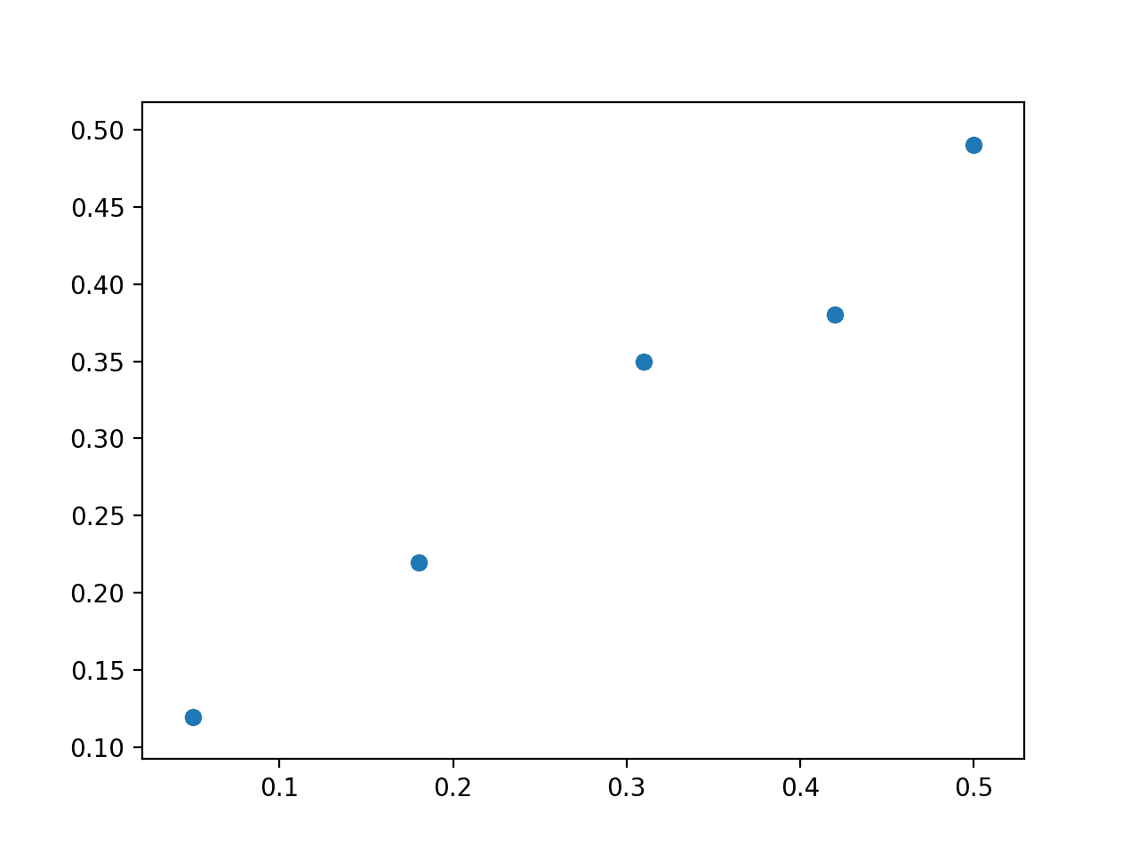
Scatter Plot of Linear Regression Dataset
Solve Directly
The first approach is to attempt to solve the regression problem directly.
That is, given X, what are the set of coefficients b that when multiplied by X will give y. As we saw in a previous section, the normal equations define how to calculate b directly.
|
1 |
b = (X^T . X)^-1 . X^T . y |
This can be calculated directly in NumPy using the inv() function for calculating the matrix inverse.
|
1 |
b = inv(X.T.dot(X)).dot(X.T).dot(y) |
Once the coefficients are calculated, we can use them to predict outcomes given X.
|
1 |
yhat = X.dot(b) |
Putting this together with the dataset defined in the previous section, the complete example is listed below.
|
1 2 3 4 5 6 7 8 9 10 11 12 13 14 15 16 17 18 19 20 21 22 |
# solve directly from numpy import array from numpy.linalg import inv from matplotlib import pyplot data = array([ [0.05, 0.12], [0.18, 0.22], [0.31, 0.35], [0.42, 0.38], [0.5, 0.49], ]) X, y = data[:,0], data[:,1] X = X.reshape((len(X), 1)) # linear least squares b = inv(X.T.dot(X)).dot(X.T).dot(y) print(b) # predict using coefficients yhat = X.dot(b) # plot data and predictions pyplot.scatter(X, y) pyplot.plot(X, yhat, color='red') pyplot.show() |
Running the example performs the calculation and prints the coefficient vector b.
|
1 |
[ 1.00233226] |
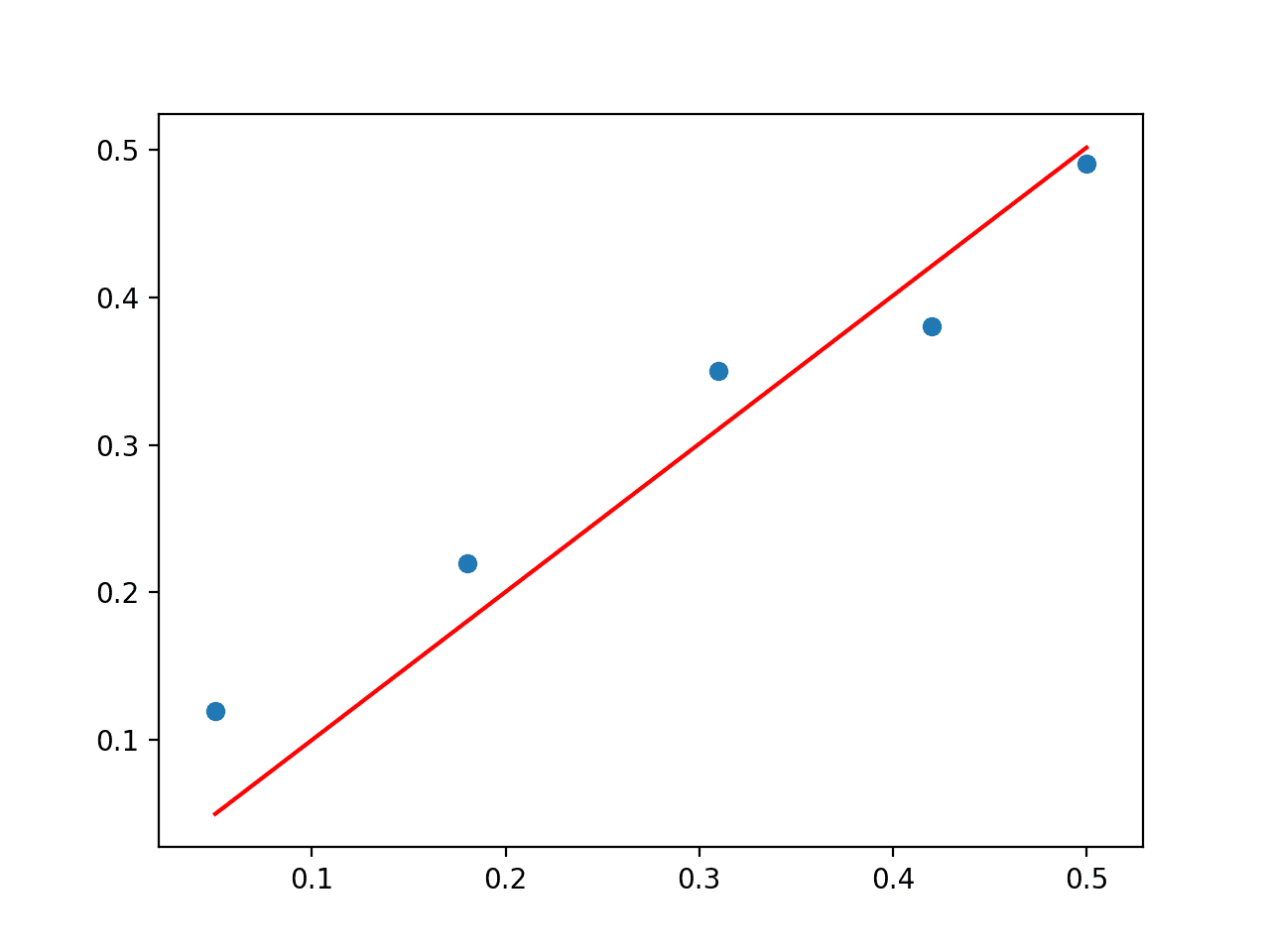
A scatter plot of the dataset is then created with a line plot for the model, showing a reasonable fit to the data.

Scatter Plot of Direct Solution to the Linear Regression Problem
A problem with this approach is the matrix inverse that is both computationally expensive and numerically unstable. An alternative approach is to use a matrix decomposition to avoid this operation. We will look at two examples in the following sections.
Solve via QR Decomposition
The QR decomposition is an approach of breaking a matrix down into its constituent elements.
|
1 |
A = Q . R |
Where A is the matrix that we wish to decompose, Q a matrix with the size m x m, and R is an upper triangle matrix with the size m x n.
The QR decomposition is a popular approach for solving the linear least squares equation.
Stepping over all of the derivation, the coefficients can be found using the Q and R elements as follows:
|
1 |
b = R^-1 . Q.T . y |
The approach still involves a matrix inversion, but in this case only on the simpler R matrix.
The QR decomposition can be found using the qr() function in NumPy. The calculation of the coefficients in NumPy looks as follows:
|
1 2 3 |
# QR decomposition Q, R = qr(X) b = inv(R).dot(Q.T).dot(y) |
Tying this together with the dataset, the complete example is listed below.
|
1 2 3 4 5 6 7 8 9 10 11 12 13 14 15 16 17 18 19 20 21 22 23 24 |
# least squares via QR decomposition from numpy import array from numpy.linalg import inv from numpy.linalg import qr from matplotlib import pyplot data = array([ [0.05, 0.12], [0.18, 0.22], [0.31, 0.35], [0.42, 0.38], [0.5, 0.49], ]) X, y = data[:,0], data[:,1] X = X.reshape((len(X), 1)) # QR decomposition Q, R = qr(X) b = inv(R).dot(Q.T).dot(y) print(b) # predict using coefficients yhat = X.dot(b) # plot data and predictions pyplot.scatter(X, y) pyplot.plot(X, yhat, color='red') pyplot.show() |
Running the example first prints the coefficient solution and plots the data with the model.
|
1 |
[ 1.00233226] |
The QR decomposition approach is more computationally efficient and more numerically stable than calculating the normal equation directly, but does not work for all data matrices.
Scatter Plot of QR Decomposition Solution to the Linear Regression Problem
Solve via Singular-Value Decomposition
The Singular-Value Decomposition, or SVD for short, is a matrix decomposition method like the QR decomposition.
|
1 |
X = U . Sigma . V^* |
Where A is the real n x m matrix that we wish to decompose, U is a m x m matrix, Sigma (often represented by the uppercase Greek letter Sigma) is an m x n diagonal matrix, and V^* is the conjugate transpose of an n x n matrix where * is a superscript.
Unlike the QR decomposition, all matrices have an SVD decomposition. As a basis for solving the system of linear equations for linear regression, SVD is more stable and the preferred approach.
Once decomposed, the coefficients can be found by calculating the pseudoinverse of the input matrix X and multiplying that by the output vector y.
|
1 |
b = X^+ . y |
Where the pseudoinverse is calculated as following:
|
1 |
X^+ = U . D^+ . V^T |
Where X^+ is the pseudoinverse of X and the + is a superscript, D^+ is the pseudoinverse of the diagonal matrix Sigma and V^T is the transpose of V^*.
Matrix inversion is not defined for matrices that are not square. […] When A has more columns than rows, then solving a linear equation using the pseudoinverse provides one of the many possible solutions.
— Page 46, Deep Learning, 2016.
We can get U and V from the SVD operation. D^+ can be calculated by creating a diagonal matrix from Sigma and calculating the reciprocal of each non-zero element in Sigma.
|
1 2 3 4 5 6 7 |
s11, 0, 0 Sigma = ( 0, s22, 0) 0, 0, s33 1/s11, 0, 0 D = ( 0, 1/s22, 0) 0, 0, 1/s33 |
We can calculate the SVD, then the pseudoinverse manually. Instead, NumPy provides the function pinv() that we can use directly.
The complete example is listed below.
|
1 2 3 4 5 6 7 8 9 10 11 12 13 14 15 16 17 18 19 20 21 22 |
# least squares via SVD with pseudoinverse from numpy import array from numpy.linalg import pinv from matplotlib import pyplot data = array([ [0.05, 0.12], [0.18, 0.22], [0.31, 0.35], [0.42, 0.38], [0.5, 0.49], ]) X, y = data[:,0], data[:,1] X = X.reshape((len(X), 1)) # calculate coefficients b = pinv(X).dot(y) print(b) # predict using coefficients yhat = X.dot(b) # plot data and predictions pyplot.scatter(X, y) pyplot.plot(X, yhat, color='red') pyplot.show() |
Running the example prints the coefficient and plots the data with a red line showing the predictions from the model.
|
1 |
[ 1.00233226] |
In fact, NumPy provides a function to replace these two steps in the lstsq() function that you can use directly.

Scatter Plot of SVD Solution to the Linear Regression Problem
Extensions
This section lists some ideas for extending the tutorial that you may wish to explore.
- Implement linear regression using the built-in lstsq() NumPy function
- Test each linear regression on your own small contrived dataset.
- Load a tabular dataset and test each linear regression method and compare the results.
If you explore any of these extensions, I’d love to know.
Further Reading
This section provides more resources on the topic if you are looking to go deeper.
Books
- Section 7.7 Least squares approximate solutions. No Bullshit Guide To Linear Algebra, 2017.
- Section 4.3 Least Squares Approximations, Introduction to Linear Algebra, Fifth Edition, 2016.
- Lecture 11, Least Squares Problems, Numerical Linear Algebra, 1997.
- Chapter 5, Orthogonalization and Least Squares, Matrix Computations, 2012.
- Chapter 12, Singular-Value and Jordan Decompositions, Linear Algebra and Matrix Analysis for Statistics, 2014.
- Section 2.9 The Moore-Penrose Pseudoinverse, Deep Learning, 2016.
- Section 15.4 General Linear Least Squares, Numerical Recipes: The Art of Scientific Computing, Third Edition, 2007.
API
- numpy.linalg.inv() API
- numpy.linalg.qr() API
- numpy.linalg.svd() API
- numpy.diag() API
- numpy.linalg.pinv() API
- numpy.linalg.lstsq() API
Articles
- Linear regression on Wikipedia
- Least squares on Wikipedia
- Linear least squares (mathematics) on Wikipedia
- Overdetermined system on Wikipedia
- QR decomposition on Wikipedia
- Singular-value decomposition on Wikipedia
- Moore–Penrose inverse
Tutorials
Summary
In this tutorial, you discovered the matrix formulation of linear regression and how to solve it using direct and matrix factorization methods.
Specifically, you learned:
- Linear regression and the matrix reformulation with the normal equations.
- How to solve linear regression using a QR matrix decomposition.
- How to solve linear regression using SVD and the pseudoinverse.
Do you have any questions?
Ask your questions in the comments below and I will do my best to answer.
Get a Handle on Linear Algebra for Machine Learning!

Develop a working understand of linear algebra
...by writing lines of code in python
Discover how in my new Ebook:
Linear Algebra for Machine Learning
It provides self-study tutorials on topics like:
Vector Norms, Matrix Multiplication, Tensors, Eigendecomposition, SVD, PCA and much more...
Finally Understand the Mathematics of Data
Skip the Academics. Just Results.


In your introduction you refer to the univariate problem, y=b0+b1*x, or Y=X.b in matrix notation. It is clear that b is a 2×1 matrix, so X has to be a nx2 matrix.
However, in your implementation of the various methods of solution you implicitly assume that b0 = 0 and then X is a nx1 matrix and b a 1×1 matrix.
For the example dataset you have chosen, this leads to a plausible solution of b1=1.00233, with a sum of squared deviations of 0.00979 and the fitted line looks more or less OK. But it is definitely not a least squares solution for the data set.
If you fit for b0 as well, you get a slope of b1= 0.78715 and b0=0.08215, with the sum of squared deviations of 0.00186. To do this, the X matrix has to be augmented with a column of ones.
If the data set had been
data = array([
[5.05, 0.12],
[5.18, 0.22],
[5.31, 0.35],
[5.42, 0.38],
[5.5, 0.49],
])
then fitting for b0 and b1 would give b1=0.78715 as before but using your formalism b1 becomes 0.05963 with sums of squared deviations of 0.00186 as before for the 2-parameter fit, but 0.07130 in your case.
Your presentation is generally quite clear, but I think it is misleading nevertheless in suggesting that it leads to a least squares solution.
Thanks John.
Hi Jason,
Thank you very much for this great and very helpful article!!!
I wonder how this method can work for quadratic curve fitting, such as parabola?
You can use a linear model with inputs raised to exponents, e.g, x^2, x^3, etc. E.g. polynomial regression.
You are too much. I need more. I would like to tell you that you are excellent in this area. More from you .Thanks.
Thanks!
Hi Jason,
I have two questions:
Does the coefficient b is always a singular value? I thought it should be a vector containing the coefficients for each Xi.
Also, can this example be applied to fit for example two parallel lines?
It is a vector of coefficients if you have a vector of inputs.
e.g. yhat = X . b
Hi Jason,
Thank you so much for all the encyclopedia of machine learning you built so far, it is really helpful 🙂
I have one question: when using sklearn’s Linear Regression on the same dataset you generated, the reg.coef_ outputs “0.78715288” instead of “1.00233226” as this algorithm did for b.
I’ve passed X and y the same way you did here and I’m quite sure they also use the pseudoinverse. Do you have any ideas why this has happened?
Minor differences in the way they perform the calculation may give slightly different coefficients/results.
The sklearn library is developed to be robust to many situations, I would expect they have made useful changes to the base method along these lines.
Hi Arthur,
This is not a minor difference and has nothing to do with the robustness of scikit-learn.
The difference is that scikit-learn’s Linear Regression model includes the intercept, whereas Jason is not here. If you want to omit this term and still get the same result for b as in scikit-learn (0.78715288), you need to subtract the mean from X and y before solving the linear regression model.
Cheers,
Yes, the intercept just centers the data, so to speak. Like a data prep.
Hi Jason,
great tutorial. I am solving a problem where my linear regression can be vertical (for example x = 3). For this problem y = X . b does not work. Do you have any ideas how to solve the problem of vertical lines?
Do you mean columns of data?
Typically a column represents many observations/samples.
Perhaps rotate your data so that a column becomes a row and can be fed into the method?
I want to know that is it possible to extract coefficients from weights of Deep learning algorithms like Convolutional Neural Networks (CNN) or Autoencoders?
You can retrieve and save the model weights directly from a neural net.
you’re right. but I have another issue.
The goal is to model choice in terms of x1 to x3 and recover the true values of beta1 to beta3 as their coefficients. V and U are unobserved
NumberOfObservations = 10000
beta1 = 4 # true values of the parameters of the model (randomly selected)
beta2 = -2
beta3 = 2
# Data generation
data = {‘ID’: pd.Series(range(1, (NumberOfObservations+1)))}
df = pd.DataFrame(data)
df[‘x1’] = np.random.normal(loc = 0, scale = 1, size = NumberOfObservations)
df[‘x2’] = np.random.normal(loc = 0, scale = 1, size = NumberOfObservations)
df[‘x3’] = np.random.normal(loc = 0, scale = 1, size = NumberOfObservations)
df[‘V1’] = beta1 * df[‘x1’] + beta2 * df[‘x2’] + beta3 * df[‘x3’]
df.loc[df[‘V1’] >=0, ‘choice’] = 1
df.loc[df[‘V1’] <0, 'choice'] = 0
for classification problems, in each layer we have several weights and in the last layer( if we have 2 classes 0 or 1) there are two weights for each Xi, how should I calculate coefficients(beta) in this case?
I believe you are describing a binary target, in this case you must use a different solution, e.g. a logistic regression – not linear regression.
Solve a linear system of equations in the form Mx = b, for the unknown
vector x, using QR factorization.in QR decomposition how to decomposition by python
See this example:
https://machinelearningmastery.com/introduction-to-matrix-decompositions-for-machine-learning/
No this is not answer my question .my question say that
Ax=b find x by qr factorization
I believe I have linked to resources that should help.
I do not have the capacity to prepare a code example for you, sorry.
Maybe I’m not the best person to help you with your project.
please give me some example about this
Diagonalize a matrix M, such that it can be written in the form D = P −1
MP,
where D is diagonal.
This tutorial shows how to calculate a diagonal matrix:
https://machinelearningmastery.com/introduction-to-types-of-matrices-in-linear-algebra/
From there, you will have enough to implement what you describe.
hi dear
in linear algebra
what is a np.linalg.pr
description by linear algebra
plz help
Perhaps you can check the API documentation directly:
https://numpy.org/doc/stable/reference/routines.linalg.html
Using numpy, for a general case of linear regression with one predictor variable and one response variable. Use matplotlib to plot a scatterplot and the fitted line. Also plot the “residuals vs fitted” graph and calculate the ????2 value. Compare your results with the R function lm() using one of Anscombe’s quartet as the dataset. You may find numpy.hstack(), np.ones() and numpy.reshape() useful.
Who understands questions like this, please?
Please I need a feedback. thanks.
adestop0072004@yahoo.ca
What is your question?