How to Implement Linear Regression From Scratch in Python

By Jason Brownlee on August 13, 2019 in Code Algorithms From Scratch 111

The core of many machine learning algorithms is optimization.

Optimization algorithms are used by machine learning algorithms to find a good set of model parameters given a training dataset.

The most common optimization algorithm used in machine learning is stochastic gradient descent.

In this tutorial, you will discover how to implement stochastic gradient descent to optimize a linear regression algorithm from scratch with Python.

After completing this tutorial, you will know:

How to estimate linear regression coefficients using stochastic gradient descent.
How to make predictions for multivariate linear regression.
How to implement linear regression with stochastic gradient descent to make predictions on new data.

Kick-start your project with my new book Machine Learning Algorithms From Scratch, including step-by-step tutorials and the Python source code files for all examples.

Let’s get started.

Update Jan/2017: Changed the calculation of fold_size in cross_validation_split() to always be an integer. Fixes issues with Python 3.
Update Aug/2018: Tested and updated to work with Python 3.6.

How to Implement Linear Regression With Stochastic Gradient Descent From Scratch With Python
Photos by star5112, some rights reserved.

Description

In this section, we will describe linear regression, the stochastic gradient descent technique and the wine quality dataset used in this tutorial.

Multivariate Linear Regression

Linear regression is a technique for predicting a real value.

Confusingly, these problems where a real value is to be predicted are called regression problems.

Linear regression is a technique where a straight line is used to model the relationship between input and output values. In more than two dimensions, this straight line may be thought of as a plane or hyperplane.

Predictions are made as a combination of the input values to predict the output value.

Each input attribute (x) is weighted using a coefficient (b), and the goal of the learning algorithm is to discover a set of coefficients that results in good predictions (y).

y = b0 + b1 * x1 + b2 * x2 + ...

1	y = b0 + b1 * x1 + b2 * x2 + ...

Coefficients can be found using stochastic gradient descent.

Stochastic Gradient Descent

Gradient Descent is the process of minimizing a function by following the gradients of the cost function.

This involves knowing the form of the cost as well as the derivative so that from a given point you know the gradient and can move in that direction, e.g. downhill towards the minimum value.

In machine learning, we can use a technique that evaluates and updates the coefficients every iteration called stochastic gradient descent to minimize the error of a model on our training data.

The way this optimization algorithm works is that each training instance is shown to the model one at a time. The model makes a prediction for a training instance, the error is calculated and the model is updated in order to reduce the error for the next prediction. This process is repeated for a fixed number of iterations.

This procedure can be used to find the set of coefficients in a model that result in the smallest error for the model on the training data. Each iteration, the coefficients (b) in machine learning language are updated using the equation:

b = b - learning_rate * error * x

1	b = b - learning_rate * error * x

Where b is the coefficient or weight being optimized, learning_rate is a learning rate that you must configure (e.g. 0.01), error is the prediction error for the model on the training data attributed to the weight, and x is the input value.

Wine Quality Dataset

After we develop our linear regression algorithm with stochastic gradient descent, we will use it to model the wine quality dataset.

This dataset is comprised of the details of 4,898 white wines including measurements like acidity and pH. The goal is to use these objective measures to predict the wine quality on a scale between 0 and 10.

Below is a sample of the first 5 records from this dataset.

7,0.27,0.36,20.7,0.045,45,170,1.001,3,0.45,8.8,6
6.3,0.3,0.34,1.6,0.049,14,132,0.994,3.3,0.49,9.5,6
8.1,0.28,0.4,6.9,0.05,30,97,0.9951,3.26,0.44,10.1,6
7.2,0.23,0.32,8.5,0.058,47,186,0.9956,3.19,0.4,9.9,6
7.2,0.23,0.32,8.5,0.058,47,186,0.9956,3.19,0.4,9.9,6

7,0.27,0.36,20.7,0.045,45,170,1.001,3,0.45,8.8,6

6.3,0.3,0.34,1.6,0.049,14,132,0.994,3.3,0.49,9.5,6

8.1,0.28,0.4,6.9,0.05,30,97,0.9951,3.26,0.44,10.1,6

7.2,0.23,0.32,8.5,0.058,47,186,0.9956,3.19,0.4,9.9,6

The dataset must be normalized to the values between 0 and 1 as each attribute has different units and in turn different scales.

By predicting the mean value (Zero Rule Algorithm) on the normalized dataset, a baseline root mean squared error (RMSE) of 0.148 can be achieved.

You can learn more about the dataset on the UCI Machine Learning Repository.

You can download the dataset and save it in your current working directory with the name winequality-white.csv. You must remove the header information from the start of the file, and convert the “;” value separator to “,” to meet CSV format.

Tutorial

This tutorial is broken down into 3 parts:

Making Predictions.
Estimating Coefficients.
Wine Quality Prediction.

This will provide the foundation you need to implement and apply linear regression with stochastic gradient descent on your own predictive modeling problems.

1. Making Predictions

The first step is to develop a function that can make predictions.

This will be needed both in the evaluation of candidate coefficient values in stochastic gradient descent and after the model is finalized and we wish to start making predictions on test data or new data.

Below is a function named predict() that predicts an output value for a row given a set of coefficients.

The first coefficient in is always the intercept, also called the bias or b0 as it is standalone and not responsible for a specific input value.

# Make a prediction with coefficients
def predict(row, coefficients):
	yhat = coefficients[0]
	for i in range(len(row)-1):
		yhat += coefficients[i + 1] * row[i]
	return yhat

# Make a prediction with coefficients

def predict(row, coefficients):

yhat = coefficients[0]

for i in range(len(row)-1):

yhat += coefficients[i + 1] * row[i]

return yhat

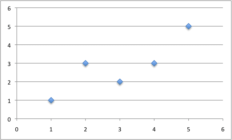
We can contrive a small dataset to test our prediction function.

x, y
1, 1
2, 3
4, 3
3, 2
5, 5

x, y

1, 1

2, 3

4, 3

3, 2

5, 5

Below is a plot of this dataset.

Small Contrived Dataset For Simple Linear Regression

Small Contrived Dataset For Linear Regression

We can also use previously prepared coefficients to make predictions for this dataset.

Putting this all together we can test our predict() function below.

# Make a prediction with coefficients
def predict(row, coefficients):
	yhat = coefficients[0]
	for i in range(len(row)-1):
		yhat += coefficients[i + 1] * row[i]
	return yhat

dataset = [[1, 1], [2, 3], [4, 3], [3, 2], [5, 5]]
coef = [0.4, 0.8]
for row in dataset:
	yhat = predict(row, coef)
	print("Expected=%.3f, Predicted=%.3f" % (row[-1], yhat))

# Make a prediction with coefficients

def predict(row, coefficients):

yhat = coefficients[0]

for i in range(len(row)-1):

yhat += coefficients[i + 1] * row[i]

return yhat

dataset = [[1, 1], [2, 3], [4, 3], [3, 2], [5, 5]]

coef = [0.4, 0.8]

for row in dataset:

yhat = predict(row, coef)

print("Expected=%.3f, Predicted=%.3f" % (row[-1], yhat))

There is a single input value (x) and two coefficient values (b0 and b1). The prediction equation we have modeled for this problem is:

y = b0 + b1 * x

1	y = b0 + b1 * x

or, with the specific coefficient values we chose by hand as:

y = 0.4 + 0.8 * x

1	y = 0.4 + 0.8 * x

Running this function we get predictions that are reasonably close to the expected output (y) values.

Expected=1.000, Predicted=1.200
Expected=3.000, Predicted=2.000
Expected=3.000, Predicted=3.600
Expected=2.000, Predicted=2.800
Expected=5.000, Predicted=4.400

Expected=1.000, Predicted=1.200

Expected=3.000, Predicted=2.000

Expected=3.000, Predicted=3.600

Expected=2.000, Predicted=2.800

Expected=5.000, Predicted=4.400

Now we are ready to implement stochastic gradient descent to optimize our coefficient values.

2. Estimating Coefficients

We can estimate the coefficient values for our training data using stochastic gradient descent.

Stochastic gradient descent requires two parameters:

Learning Rate: Used to limit the amount each coefficient is corrected each time it is updated.
Epochs: The number of times to run through the training data while updating the coefficients.

These, along with the training data will be the arguments to the function.

There are 3 loops we need to perform in the function:

Loop over each epoch.
Loop over each row in the training data for an epoch.
Loop over each coefficient and update it for a row in an epoch.

As you can see, we update each coefficient for each row in the training data, each epoch.

Coefficients are updated based on the error the model made. The error is calculated as the difference between the prediction made with the candidate coefficients and the expected output value.

error = prediction - expected

1	error = prediction - expected

There is one coefficient to weight each input attribute, and these are updated in a consistent way, for example:

b1(t+1) = b1(t) - learning_rate * error(t) * x1(t)

1	b1(t+1) = b1(t) - learning_rate * error(t) * x1(t)

The special coefficient at the beginning of the list, also called the intercept or the bias, is updated in a similar way, except without an input as it is not associated with a specific input value:

b0(t+1) = b0(t) - learning_rate * error(t)

1	b0(t+1) = b0(t) - learning_rate * error(t)

Now we can put all of this together. Below is a function named coefficients_sgd() that calculates coefficient values for a training dataset using stochastic gradient descent.

# Estimate linear regression coefficients using stochastic gradient descent
def coefficients_sgd(train, l_rate, n_epoch):
	coef = [0.0 for i in range(len(train[0]))]
	for epoch in range(n_epoch):
		sum_error = 0
		for row in train:
			yhat = predict(row, coef)
			error = yhat - row[-1]
			sum_error += error**2
			coef[0] = coef[0] - l_rate * error
			for i in range(len(row)-1):
				coef[i + 1] = coef[i + 1] - l_rate * error * row[i]
		print('>epoch=%d, lrate=%.3f, error=%.3f' % (epoch, l_rate, sum_error))
	return coef

# Estimate linear regression coefficients using stochastic gradient descent

def coefficients_sgd(train, l_rate, n_epoch):

coef = [0.0 for i in range(len(train[0]))]

for epoch in range(n_epoch):

sum_error = 0

for row in train:

yhat = predict(row, coef)

error = yhat - row[-1]

sum_error += error**2

coef[0] = coef[0] - l_rate * error

for i in range(len(row)-1):

coef[i + 1] = coef[i + 1] - l_rate * error * row[i]

print('>epoch=%d, lrate=%.3f, error=%.3f' % (epoch, l_rate, sum_error))

return coef

You can see, that in addition, we keep track of the sum of the squared error (a positive value) each epoch so that we can print out a nice message in the outer loop.

We can test this function on the same small contrived dataset from above.

# Make a prediction with coefficients
def predict(row, coefficients):
	yhat = coefficients[0]
	for i in range(len(row)-1):
		yhat += coefficients[i + 1] * row[i]
	return yhat

# Estimate linear regression coefficients using stochastic gradient descent
def coefficients_sgd(train, l_rate, n_epoch):
	coef = [0.0 for i in range(len(train[0]))]
	for epoch in range(n_epoch):
		sum_error = 0
		for row in train:
			yhat = predict(row, coef)
			error = yhat - row[-1]
			sum_error += error**2
			coef[0] = coef[0] - l_rate * error
			for i in range(len(row)-1):
				coef[i + 1] = coef[i + 1] - l_rate * error * row[i]
		print('>epoch=%d, lrate=%.3f, error=%.3f' % (epoch, l_rate, sum_error))
	return coef

# Calculate coefficients
dataset = [[1, 1], [2, 3], [4, 3], [3, 2], [5, 5]]
l_rate = 0.001
n_epoch = 50
coef = coefficients_sgd(dataset, l_rate, n_epoch)
print(coef)

# Make a prediction with coefficients

def predict(row, coefficients):

yhat = coefficients[0]

for i in range(len(row)-1):

yhat += coefficients[i + 1] * row[i]

return yhat

# Estimate linear regression coefficients using stochastic gradient descent

def coefficients_sgd(train, l_rate, n_epoch):

coef = [0.0 for i in range(len(train[0]))]

for epoch in range(n_epoch):

sum_error = 0

for row in train:

yhat = predict(row, coef)

error = yhat - row[-1]

sum_error += error**2

coef[0] = coef[0] - l_rate * error

for i in range(len(row)-1):

coef[i + 1] = coef[i + 1] - l_rate * error * row[i]

print('>epoch=%d, lrate=%.3f, error=%.3f' % (epoch, l_rate, sum_error))

return coef

# Calculate coefficients

dataset = [[1, 1], [2, 3], [4, 3], [3, 2], [5, 5]]

l_rate = 0.001

n_epoch = 50

coef = coefficients_sgd(dataset, l_rate, n_epoch)

print(coef)

We use a small learning rate of 0.001 and train the model for 50 epochs, or 50 exposures of the coefficients to the entire training dataset.

Running the example prints a message each epoch with the sum squared error for that epoch and the final set of coefficients.

>epoch=45, lrate=0.001, error=2.650
>epoch=46, lrate=0.001, error=2.627
>epoch=47, lrate=0.001, error=2.607
>epoch=48, lrate=0.001, error=2.589
>epoch=49, lrate=0.001, error=2.573
[0.22998234937311363, 0.8017220304137576]

>epoch=45, lrate=0.001, error=2.650

>epoch=46, lrate=0.001, error=2.627

>epoch=47, lrate=0.001, error=2.607

>epoch=48, lrate=0.001, error=2.589

>epoch=49, lrate=0.001, error=2.573

[0.22998234937311363, 0.8017220304137576]

You can see how error continues to drop even in the final epoch. We could probably train for a lot longer (more epochs) or increase the amount we update the coefficients each epoch (higher learning rate).

Experiment and see what you come up with.

Now, let’s apply this algorithm on a real dataset.

3. Wine Quality Prediction

In this section, we will train a linear regression model using stochastic gradient descent on the wine quality dataset.

The example assumes that a CSV copy of the dataset is in the current working directory with the filename winequality-white.csv.

The dataset is first loaded, the string values converted to numeric and each column is normalized to values in the range of 0 to 1. This is achieved with helper functions load_csv() and str_column_to_float() to load and prepare the dataset and dataset_minmax() and normalize_dataset() to normalize it.

We will use k-fold cross-validation to estimate the performance of the learned model on unseen data. This means that we will construct and evaluate k models and estimate the performance as the mean model error. Root mean squared error will be used to evaluate each model. These behaviors are provided in the cross_validation_split(), rmse_metric() and evaluate_algorithm() helper functions.

We will use the predict(), coefficients_sgd() and linear_regression_sgd() functions created above to train the model.

Below is the complete example.

# Linear Regression With Stochastic Gradient Descent for Wine Quality
from random import seed
from random import randrange
from csv import reader
from math import sqrt

# Load a CSV file
def load_csv(filename):
	dataset = list()
	with open(filename, 'r') as file:
		csv_reader = reader(file)
		for row in csv_reader:
			if not row:
				continue
			dataset.append(row)
	return dataset

# Convert string column to float
def str_column_to_float(dataset, column):
	for row in dataset:
		row[column] = float(row[column].strip())

# Find the min and max values for each column
def dataset_minmax(dataset):
	minmax = list()
	for i in range(len(dataset[0])):
		col_values = [row[i] for row in dataset]
		value_min = min(col_values)
		value_max = max(col_values)
		minmax.append([value_min, value_max])
	return minmax

# Rescale dataset columns to the range 0-1
def normalize_dataset(dataset, minmax):
	for row in dataset:
		for i in range(len(row)):
			row[i] = (row[i] - minmax[i][0]) / (minmax[i][1] - minmax[i][0])

# Split a dataset into k folds
def cross_validation_split(dataset, n_folds):
	dataset_split = list()
	dataset_copy = list(dataset)
	fold_size = int(len(dataset) / n_folds)
	for i in range(n_folds):
		fold = list()
		while len(fold) < fold_size:
			index = randrange(len(dataset_copy))
			fold.append(dataset_copy.pop(index))
		dataset_split.append(fold)
	return dataset_split

# Calculate root mean squared error
def rmse_metric(actual, predicted):
	sum_error = 0.0
	for i in range(len(actual)):
		prediction_error = predicted[i] - actual[i]
		sum_error += (prediction_error ** 2)
	mean_error = sum_error / float(len(actual))
	return sqrt(mean_error)

# Evaluate an algorithm using a cross validation split
def evaluate_algorithm(dataset, algorithm, n_folds, *args):
	folds = cross_validation_split(dataset, n_folds)
	scores = list()
	for fold in folds:
		train_set = list(folds)
		train_set.remove(fold)
		train_set = sum(train_set, [])
		test_set = list()
		for row in fold:
			row_copy = list(row)
			test_set.append(row_copy)
			row_copy[-1] = None
		predicted = algorithm(train_set, test_set, *args)
		actual = [row[-1] for row in fold]
		rmse = rmse_metric(actual, predicted)
		scores.append(rmse)
	return scores

# Make a prediction with coefficients
def predict(row, coefficients):
	yhat = coefficients[0]
	for i in range(len(row)-1):
		yhat += coefficients[i + 1] * row[i]
	return yhat

# Estimate linear regression coefficients using stochastic gradient descent
def coefficients_sgd(train, l_rate, n_epoch):
	coef = [0.0 for i in range(len(train[0]))]
	for epoch in range(n_epoch):
		for row in train:
			yhat = predict(row, coef)
			error = yhat - row[-1]
			coef[0] = coef[0] - l_rate * error
			for i in range(len(row)-1):
				coef[i + 1] = coef[i + 1] - l_rate * error * row[i]
			# print(l_rate, n_epoch, error)
	return coef

# Linear Regression Algorithm With Stochastic Gradient Descent
def linear_regression_sgd(train, test, l_rate, n_epoch):
	predictions = list()
	coef = coefficients_sgd(train, l_rate, n_epoch)
	for row in test:
		yhat = predict(row, coef)
		predictions.append(yhat)
	return(predictions)

# Linear Regression on wine quality dataset
seed(1)
# load and prepare data
filename = 'winequality-white.csv'
dataset = load_csv(filename)
for i in range(len(dataset[0])):
	str_column_to_float(dataset, i)
# normalize
minmax = dataset_minmax(dataset)
normalize_dataset(dataset, minmax)
# evaluate algorithm
n_folds = 5
l_rate = 0.01
n_epoch = 50
scores = evaluate_algorithm(dataset, linear_regression_sgd, n_folds, l_rate, n_epoch)
print('Scores: %s' % scores)
print('Mean RMSE: %.3f' % (sum(scores)/float(len(scores))))

100

101

102

103

104

105

106

107

108

109

110

111

112

113

114

115

116

117

118

119

120

121

122

123

124

125

# Linear Regression With Stochastic Gradient Descent for Wine Quality

from random import seed

from random import randrange

from csv import reader

from math import sqrt

# Load a CSV file

def load_csv(filename):

dataset = list()

with open(filename, 'r') as file:

csv_reader = reader(file)

for row in csv_reader:

if not row:

continue

dataset.append(row)

return dataset

# Convert string column to float

def str_column_to_float(dataset, column):

for row in dataset:

row[column] = float(row[column].strip())

# Find the min and max values for each column

def dataset_minmax(dataset):

minmax = list()

for i in range(len(dataset[0])):

col_values = [row[i] for row in dataset]

value_min = min(col_values)

value_max = max(col_values)

minmax.append([value_min, value_max])

return minmax

# Rescale dataset columns to the range 0-1

def normalize_dataset(dataset, minmax):

for row in dataset:

for i in range(len(row)):

row[i] = (row[i] - minmax[i][0]) / (minmax[i][1] - minmax[i][0])

# Split a dataset into k folds

def cross_validation_split(dataset, n_folds):

dataset_split = list()

dataset_copy = list(dataset)

fold_size = int(len(dataset) / n_folds)

for i in range(n_folds):

fold = list()

while len(fold) < fold_size:

index = randrange(len(dataset_copy))

fold.append(dataset_copy.pop(index))

dataset_split.append(fold)

return dataset_split

# Calculate root mean squared error

def rmse_metric(actual, predicted):

sum_error = 0.0

for i in range(len(actual)):

prediction_error = predicted[i] - actual[i]

sum_error += (prediction_error ** 2)

mean_error = sum_error / float(len(actual))

return sqrt(mean_error)

# Evaluate an algorithm using a cross validation split

def evaluate_algorithm(dataset, algorithm, n_folds, *args):

folds = cross_validation_split(dataset, n_folds)

scores = list()

for fold in folds:

train_set = list(folds)

train_set.remove(fold)

train_set = sum(train_set, [])

test_set = list()

for row in fold:

row_copy = list(row)

test_set.append(row_copy)

row_copy[-1] = None

predicted = algorithm(train_set, test_set, *args)

actual = [row[-1] for row in fold]

rmse = rmse_metric(actual, predicted)

scores.append(rmse)

return scores

# Make a prediction with coefficients

def predict(row, coefficients):

yhat = coefficients[0]

for i in range(len(row)-1):

yhat += coefficients[i + 1] * row[i]

return yhat

# Estimate linear regression coefficients using stochastic gradient descent

def coefficients_sgd(train, l_rate, n_epoch):

coef = [0.0 for i in range(len(train[0]))]

for epoch in range(n_epoch):

for row in train:

yhat = predict(row, coef)

error = yhat - row[-1]

coef[0] = coef[0] - l_rate * error

for i in range(len(row)-1):

coef[i + 1] = coef[i + 1] - l_rate * error * row[i]

# print(l_rate, n_epoch, error)

return coef

# Linear Regression Algorithm With Stochastic Gradient Descent

def linear_regression_sgd(train, test, l_rate, n_epoch):

predictions = list()

coef = coefficients_sgd(train, l_rate, n_epoch)

for row in test:

yhat = predict(row, coef)

predictions.append(yhat)

return(predictions)

# Linear Regression on wine quality dataset

seed(1)

# load and prepare data

filename = 'winequality-white.csv'

dataset = load_csv(filename)

for i in range(len(dataset[0])):

str_column_to_float(dataset, i)

# normalize

minmax = dataset_minmax(dataset)

normalize_dataset(dataset, minmax)

# evaluate algorithm

n_folds = 5

l_rate = 0.01

n_epoch = 50

scores = evaluate_algorithm(dataset, linear_regression_sgd, n_folds, l_rate, n_epoch)

print('Scores: %s' % scores)

print('Mean RMSE: %.3f' % (sum(scores)/float(len(scores))))

A k value of 5 was used for cross-validation, giving each fold 4,898/5 = 979.6 or just under 1000 records to be evaluated upon each iteration. A learning rate of 0.01 and 50 training epochs were chosen with a little experimentation.

You can try your own configurations and see if you can beat my score.

Running this example prints the scores for each of the 5 cross-validation folds then prints the mean RMSE.

We can see that the RMSE (on the normalized dataset) is 0.126, lower than the baseline value of 0.148 if we just predicted the mean (using the Zero Rule Algorithm).

Scores: [0.12248058224159092, 0.13034017509167112, 0.12620370547483578, 0.12897687952843237, 0.12446990678682233]
Mean RMSE: 0.126

1 2	Scores: [0.12248058224159092, 0.13034017509167112, 0.12620370547483578, 0.12897687952843237, 0.12446990678682233] Mean RMSE: 0.126

Extensions

This section lists a number of extensions to this tutorial that you may wish to consider exploring.

Tune The Example. Tune the learning rate, number of epochs and even the data preparation method to get an improved score on the wine quality dataset.
Batch Stochastic Gradient Descent. Change the stochastic gradient descent algorithm to accumulate updates across each epoch and only update the coefficients in a batch at the end of the epoch.
Additional Regression Problems. Apply the technique to other regression problems on the UCI machine learning repository.

Did you explore any of these extensions?
Let me know about it in the comments below.

Review

In this tutorial, you discovered how to implement linear regression using stochastic gradient descent from scratch with Python.

You learned.

How to make predictions for a multivariate linear regression problem.
How to optimize a set of coefficients using stochastic gradient descent.
How to apply the technique to a real regression predictive modeling problem.

Do you have any questions?
Ask your question in the comments below and I will do my best to answer.

111 Responses to How to Implement Linear Regression From Scratch in Python

Blessing Ojeme October 28, 2016 at 11:41 am #

Thanks, Jason, for keeping it as simple and straight as it can be. The tutorial was quite helpful.

Reply
- Jason Brownlee October 28, 2016 at 12:00 pm #
  
  I’m glad to hear that Blessing.
  
  Reply
Arvind Ganesh March 12, 2017 at 8:47 pm #

Are you handpicking the coefficients so that you have something to go off of for training? Why don’t you just use random values for the coefficients, and then go directly into gradient descent?

Reply
- Jason Brownlee March 13, 2017 at 7:41 am #
  
  In the final example (end of the tutorial), I use the initial coefficients of “0” and use SGD to search for coefficients that best fit the data.
  
  Reply
  - Christian Picon Calderon September 10, 2019 at 1:33 pm #
    
    you are feed the sdg with the label of the test (line 70 -74):
    
    for row in fold: row_copy = list(row) test_set.append(row_copy) row_copy[-1] = None <<<<-- it must before
    
    1
    2
    3
    4
    
    for row in fold:
    row_copy = list(row)
    test_set.append(row_copy)
    row_copy[-1] = None <<<<-- it must before
    
    Reply
    - Jason Brownlee September 10, 2019 at 2:22 pm #
      
      I don’t believe so, we are operating on the list that happens to be in the test set list.
      
      E.g. a reference to the list.
      
      Reply
klaas March 18, 2017 at 10:24 pm #

Hi Jason,

this blog is really awesome and the more i read the more questions appear. Here for instance i don’t get why the wine dataset is actually labeled as regression problem? We have fixed class labels so it should be a categorical classification right?
I would also like to know if you would recommend also standardizing the labels too or is it enough to do this with the features? Google is not totally clear about that so i prefer an expert’s opinion. Thanks

Reply
- Jason Brownlee March 19, 2017 at 6:11 am #
  
  You could treat the problem as classification, try it and see (with a different algorithm).
  
  Standardization can help. Again try it on your problem and see.
  
  Reply
Nandhini April 9, 2017 at 4:54 pm #

Hi Jason,
Have a question on finding the optimal coeff? What I understood from the equation of Gradient Descent :
coeff(0) = coeff(0) – l_rate *1\m*errors
coeff(1) = coeff(1) – l_rate * 1\m * errors * X[i]
where m is no.of training rows.

But in the above code I couldn’t figure out 1\m part. Could you explain me whats wrong in my understanding of the gradient descent equation.

Reply
- Jason Brownlee April 10, 2017 at 7:37 am #
  
  I did not include the scaling term 1/m. You can if you like.
  
  Reply
  - Adarsh September 13, 2017 at 1:58 am #
    
    I seem to get different values for my coefficients and sum_error when I incorporate 1/m. Should this be so?
    
    Reply
    - Jason Brownlee September 13, 2017 at 12:32 pm #
      
      Yes, see this post:
      https://machinelearningmastery.com/randomness-in-machine-learning/
      
      Reply
  - Gonzalo A. Aranda October 15, 2020 at 8:54 pm #
    
    The problem is the Error’s Definition… which it is NOT CORRECT!
    
    It defines as yhat – y … and this can means that 2 examples with +1 and -1 of error summarize 0 error.
    
    The correct definition would be 1/2 (yhat – y)^2 …. and in the updates, the derivation includes X_i. ….
    
    Reply
Kirill April 13, 2017 at 1:40 am #

Hi there Jason,
The problem you solving here is searching for coefficients that fitting straight line to the data. But how to visualize the result of this algorithm, is it even possible?

Reply
- Jason Brownlee April 13, 2017 at 10:06 am #
  
  Yes, you can feed in each possible input variable (x) to the learned model and collect the output variable (y), then plot the x,y points.
  
  Reply
Sri May 28, 2017 at 3:54 am #

When dealing with many inputs(>3) how do we visualize the data, because in the wine quality dataset there are 11 features/inputs.

Reply
- Jason Brownlee June 2, 2017 at 12:05 pm #
  
  You can use pair-wise scatter plots.
  
  Reply
Kay June 17, 2017 at 7:47 am #

Hi Jason,

I am working with a dataset with 6 columns per row, where the first 5 values (say, a,b,c,d,e) are input variables that produce the 6th value as an output (say, y). Now if I want to utilize SGD, as implemented above, to find a set of a,b,c,d,e that maximizes y (minimizes 1-y), how would I go about this? Thanks for your tutorials, they’re incredibly helpful for someone just starting out!

Reply
- Jason Brownlee June 18, 2017 at 6:28 am #
  
  You may want to start with a standard tool like Weka:
  https://machinelearningmastery.com/start-here/#weka
  
  Reply
Jason L June 20, 2017 at 6:23 am #

Hi Jason,

I’m applying your tutorial to a modeling scenario with 5 inputs, one output, input and output variable scale in the 10^4 to 10^5 range (it is a media modeling example estimating cost efficiency where we typically don’t normalize in pre-processing). In comparing your methods with the SKlearn linear regression, I’m finding that I can’t estimate the intercept very accurately using your method, and my coefficients and intercept all converge to some reasonably small and similar values, (initializing all coefficients as 0). When initializing the intercept term to be similar to the SKlearn linear regression intercept result, your method converges to exactly the result of SKlearn linear regression. Would you say that your method is dependent on the initialization of coefficients, and is this a phenomenon you’ve encountered before? I’m curious if I am overlooking something, or if this is dependent on the scale of the data, or if this is the result of the data having an apparently large intercept.

Reply
- Jason L June 20, 2017 at 6:42 am #
  
  I also want to note that when comparing your method to SKlearn linear regression with no intercept, it is perfect.
  
  Reply
- Jason Brownlee June 20, 2017 at 6:44 am #
  
  Gradient descent is more suitable when you cannot use the linalg methods (like sklearn) that require all data to fit into memory.
  
  The GD method may need to be tuned on your problem, e.g. learning rate, batch size, etc.
  
  Reply
nenduru July 5, 2017 at 2:14 pm #

Hi Jason

thank you for these awesome tutorials,
Are you initializing coef[0] and coef[1] = 0 in the below code?
debugging through for loops is confusing

coef = [0.0 for i in range(len(train[0]))]

Reply
- Jason Brownlee July 6, 2017 at 10:21 am #
  
  Yes, zero init.
  
  Reply
Mohit Garg August 10, 2017 at 12:05 am #

Thank u so much sir for your efforts….
Sir can u tell how to omit first row of csv file

Reply
- Jason Brownlee August 10, 2017 at 6:58 am #
  
  Some ideas:
  
  – Delete it manually
  – Skip it when loading with read_csv
  – Load it then delete it from the dataframe using pandas or from the array using numpy later.
  
  I hope that helps as a start.
  
  Reply
mohit garg August 11, 2017 at 3:23 am #

sir when i call ds.info its shows that it read it as a single column plzz can u tell how to fix this problem

this is code:

df=pd.read_csv(‘wine1.csv’)
df.info()

OUTPUT:
class ‘pandas.core.frame.DataFrame’>
RangeIndex: 4898 entries, 0 to 4897
Data columns (total 1 columns):
fixed acidity;”volatile acidity”;”citric acid”;”residual sugar”;”chlorides”;”free sulfur dioxide”;”total sulfur dioxide”;”density”;”pH”;”sulphates”;”alcohol”;”quality” 4898 non-null object
dtypes: object(1)
memory usage: 38.3+ KB

Reply
- Jason Brownlee August 11, 2017 at 6:45 am #
  
  You may need to configure the loading to separate the columns by ‘;’ instead of ‘,’.
  
  See the API here:
  https://pandas.pydata.org/pandas-docs/stable/generated/pandas.read_csv.html
  
  Reply
Arthur Grisel-DAvy August 12, 2017 at 8:32 pm #

Great tutorial thanks you.
However i find myself stuck on a problem. One of the value of the wine dataset (total sulfur dioxide) if way greater than the others and it create an unstable situation where the error and the coefficient soar, switching from positive to negative, causing an overflow. I can’t even go through 200 lines of the dataset. I checked my code and copy past yours but nothing changed.
Is this a classic issue ? Is there a simple solution ?

Reply
- Jason Brownlee August 13, 2017 at 9:53 am #
  
  Sorry to hear that.
  
  Perhaps you can identify that example and remove it from the dataset?
  
  Reply
neha August 16, 2017 at 5:28 am #

Hi Jason,
I am working on Campaign Analysis and using Linear Regression following cross validation, SGD in Python.Previously applying Linear Regression using 80% train set and 20% test set i used to get the prediction and recommend in terms of the deciles, where as in this technique recommended by you how can i divide my dataset into deciles and recommend?

Reply
- Jason Brownlee August 16, 2017 at 6:41 am #
  
  They are two different ways of estimating the skill of the model on unseen data.
  
  Use the approach that gives you the least biased estimates.
  
  Reply
  - nehasharma August 16, 2017 at 5:43 pm #
    
    So if i adopt your approach of cross validation i am getting 5 rows of Coefficients as fold =5..For my final linear regression equation which coefficients should i choose in order to finalize my equation and then derive the decile split for recommendation?
    
    Reply
    - Jason Brownlee August 17, 2017 at 6:37 am #
      
      Once you choose a model configuration, you can fit a final model on all data and use it for making predictions.
      
      More about developing a final model here:
      https://machinelearningmastery.com/train-final-machine-learning-model/
      
      Reply
      - nehasharma August 17, 2017 at 11:31 pm #
        
        Thanks for the reply!u really helped me!
      - Jason Brownlee August 18, 2017 at 6:21 am #
        
        I’m glad to hear that.
KUNAL SARKAR August 21, 2017 at 12:37 pm #

Hi Jason,
Here you are updating the weightages after every sample, but as per SGD it should be after a batch processing. Can you please explain?

Reply
- Jason Brownlee August 21, 2017 at 4:24 pm #
  
  Updating after each example is called “stochastic gradient descent”.
  
  Updating after batches of samples is called “mini-batch gradient descent”.
  
  Learn more about the differences here:
  https://machinelearningmastery.com/gentle-introduction-mini-batch-gradient-descent-configure-batch-size/
  
  Reply
Shinichi September 2, 2017 at 8:29 pm #

How can we add regularization in it, where, regularization norm is a general p-norm with 1<=p<=2 (p=1 being lasso and p=2 ridge)?

Reply
- Jason Brownlee September 3, 2017 at 5:42 am #
  
  Update the loss function to take into account the magnitude of the combined coefficients.
  
  Sorry, I do not have worked example (yet).
  
  Reply
Ami Tabak October 25, 2017 at 11:38 pm #

wont (minmax[i][1] – minmax[i][0]) will result in 0 division

Reply
- Jason Brownlee October 26, 2017 at 5:29 am #
  
  Why?
  
  Reply
  - Ami Tabak October 27, 2017 at 8:26 pm #
    
    File “C:/tutorials/pure-python-lessons/linear-regression/stochastic-regression-protect-nan.py”, line 37, in normalize_dataset
    row[i] = (row[i] – minmax[i][0]) / (minmax[i][1] – minmax[i][0])
    
    ZeroDivisionError: float division by zero
    
    The csv is
    
    7,0.27,0.36,20.7,0.045,45,170,1.001,3,0.45,8.8,6
    6.3,0.3,0.34,1.6,0.049,14,132,0.994,3.3,0.49,9.5,6
    8.1,0.28,0.4,6.9,0.05,30,97,0.9951,3.26,0.44,10.1,6
    7.2,0.23,0.32,8.5,0.058,47,186,0.9956,3.19,0.4,9.9,6
    7.2,0.23,0.32,8.5,0.058,47,186,0.9956,3.19,0.4,9.9,6
    
    Reply
    - Jason Brownlee October 28, 2017 at 5:12 am #
      
      It suggests that perhaps one of your columns has all the same value. Perhaps you can remove this column?
      
      Reply
      - Ami tabak October 28, 2017 at 5:12 pm #
        
        Hi Jason
        The data I used is from this page. You posted it as a wine quality stats.
        Indeed when I change it so the last column wont be unanimous the error no longer appears.
        
        But of course this can happen in other data sets.
        will it be correct to change the code to the following?
        
        def normalize_dataset(dataset, minmax):
        for row in dataset:
        for i in range(len(row)):
        if minmax[i][1] == minmax[i][0]:
        row[i] = 0
        else:
        row[i] = (row[i] – minmax[i][0]) / (minmax[i][1] – minmax[i][0])
      - Jason Brownlee October 29, 2017 at 5:51 am #
        
        Normally we would remove columns that have no information like the one you describe.
Imtithal Saeed May 23, 2018 at 12:41 am #

hi Jason,

So why using stochastic gradient descent? rather than others ? for example gradient descent with sum squares?

Reply
- Jason Brownlee May 23, 2018 at 6:27 am #
  
  The main reason is when the matrix of input data does not fit into memory meaning the linalg solution cannot be calculated.
  
  Reply
Prabhu June 4, 2018 at 3:36 am #

ValueError: could not convert string to float: fixed acidity;”volatile acidity”;”citric acid”;”residual sugar”;”chlorides”;”free sulfur dioxide”;”total sulfur dioxide”;”density”;”pH”;”sulphates”;”alcohol”;”quality”

Reply
- Jason Brownlee June 4, 2018 at 6:34 am #
  
  Looks like you are working with a different dataset that might need to be processed first.
  
  Reply
- Guardiana July 2, 2018 at 11:09 pm #
  
  Hey, I had the same problem. The Problem is the delimiter in the csv file. You just need to change line 11 from
  csv_reader = reader(file)
  to
  csv_reader = reader(file,delimiter=’;’)
  
  Reply
Guardiana July 3, 2018 at 12:48 am #

Hi Jason,

in Line 47, you fill you fold list with random indexed entries from the dataset. That means that some points will appear more than once in a fold, and that not every point is used, right? Wouldnt it be better to use every point?
Thanks in advance!

Reply
- Jason Brownlee July 3, 2018 at 6:27 am #
  
  Not quite, you can learn more about cross validation here:
  https://machinelearningmastery.com/k-fold-cross-validation/
  
  Reply
vince August 13, 2018 at 1:14 am #

Hi Jason,

I tried your example and all works well, however I tried to use the function to estimate the coefficients on a different dataset with negative relations between predictors and the target variable and this function does not seem to give any negative coefficients. I tried different learning rates but that is not it.

Hope you can point me in the right direction where I go wrong here.

The dataset I used is the mtcars dataset with disp and hp as examples of columns negatively correlated with mpg.

Reply
- Jason Brownlee August 13, 2018 at 6:18 am #
  
  Perhaps try scaling the data before fitting the model?
  
  Reply
vincent August 23, 2018 at 2:26 pm #

Hi Jason,
Thank you for your awesome tutorials.
I’m trying your SGD with my dataset. My dataset has 6 features a,b,c,d,e,f and g is target result which I have to predict. some rows in my dataset like this:
a b c d e f g
8 20 2 8 1 0 162401
7 30 2 16 1 0 157731
7 30 2 10 1 0 174087
7 30 2 14 1 0 175439
7 30 2 11 1 0 137424
So, my problem here is if i normalize data like this tutorial, I must normalize g column, too. and after I have coefficients vector, how can i predict the result with my test data? because the value of elements in coef vector is very small. On the other hand, the actual result of g column is very large.

Reply
- Jason Brownlee August 24, 2018 at 6:06 am #
  
  You must normalize test data as well, using the min/max from the training data.
  
  Reply
dohye September 11, 2018 at 10:08 pm #

Hi, Jason. Thank you for your explanation.

But I have one question. Could you tell me why are you using error instead of gradient?
I’m looking forward your answer.
Thank you 🙂

Reply
- Jason Brownlee September 12, 2018 at 8:11 am #
  
  We navigate down the error gradient.
  
  Reply
Ken Stpnecipher September 24, 2018 at 2:50 pm #

Jason where do you get the 0,148 number?

We can see that the RMSE (on the normalized dataset) is 0.126, lower than the baseline value of 0.148 if we just predicted the mean (using the Zero Rule Algorithm).

Thanks

Ken

Reply
- Jason Brownlee September 25, 2018 at 6:16 am #
  
  I ran an zeror on the dataset beforehand.
  
  Earlier in the tutorial I noted:
  
  By predicting the mean value (Zero Rule Algorithm) on the normalized dataset, a baseline root mean squared error (RMSE) of 0.148 can be achieved.
  
  Reply
Muath Kefayah October 19, 2018 at 7:02 pm #

Hi Jason,

In yours tutorial , what is the feature you considered as response variable (target) ?

Thanks in advance

Reply
- Jason Brownlee October 20, 2018 at 5:53 am #
  
  Wine quality.
  
  Reply
sandy October 26, 2018 at 10:43 pm #

why do not use sklearn models.why u use regular program code.is it there any difference between them and any complexity

Reply
- Jason Brownlee October 27, 2018 at 6:01 am #
  
  I recommend using sklearn in general.
  
  I show how to code it from scratch as a learning exercise only.
  
  Reply
Manjunath December 27, 2018 at 5:29 pm #

Hi,
i was trying to run or follow your steps i am getting below error
OverflowError: (34, ‘Numerical result out of range’)
in evaluate_algorithm(dataset, algorithm, n_folds, *args)
12 test_set.append(row_copy)
13 row_copy[-1] = None
—> 14 predicted = algorithm(train_set, test_set, *args)
15 actual = [row[-1] for row in fold]
16 rmse = rmse_metric(actual, predicted)

in linear_regression_sgd(train, test, l_rate, n_epoch)
21 def linear_regression_sgd(train, test, l_rate, n_epoch):
22 predictions = list()
—> 23 coef = coefficients_sgd(train, l_rate, n_epoch)
24 for row in test:
25 yhat = predict(row, coef)

in coefficients_sgd(train, l_rate, n_epoch)
35 yhat = predict(row, coef)
36 error = yhat – row[-1]
—> 37 sum_error += error**2
38 coef[0] = coef[0] – l_rate * error
39 for i in range(len(row)-1):

Reply
- Jason Brownlee December 28, 2018 at 5:53 am #
  
  I have some suggestions here:
  https://machinelearningmastery.com/faq/single-faq/why-does-the-code-in-the-tutorial-not-work-for-me
  
  Reply
Saitejapsk March 20, 2019 at 9:31 pm #

Hi i’m going to apply SGD for linear regression with sk learn’s Boston dataset can you share me some good resource like you

Reply
- Jason Brownlee March 21, 2019 at 8:09 am #
  
  This post (above) is all you really need and a great place to start.
  
  Reply
Toni April 26, 2019 at 7:17 am #

Hi Jason! Thanks for your work. A am somewhat beginner in the ML algorithms, especially in the math part of it. I am thinking all the day how you derivated the error function. I know that the error function in the code is (error = yhat – row(-1)), and yhat is taken from the function predict. From what I understand, the predict function in the math is something like (f(x) = x0 + n – 1
Σ
i = 1
xi * d(i-1)
where d is the data and n is the length. I tried to get the derivative function, but looks like I am doing it in the wrong way.

Reply
- Jason Brownlee April 26, 2019 at 8:40 am #
  
  I did not derive the error function, I used a derivation from a book.
  
  Reply
  - Toni April 27, 2019 at 5:15 pm #
    
    Thank you very much for the reply! I (after much thinking) concluded that the derived part in the code is not
    error * row(i)
    but only
    row(i)
    based on the derivation of the straight line function
    f'(x) (a + bx – y) = b
    and concluded that the gradient descent algorithm works by subtracting from the coefficients
    error * derivation * lrate
    and not
    derivation * lrate
    , but in the “Estimating Coefficients” part of the tutorial, if I change the line 19 with
    coef(i + 1) = coef(i + 1) – l_rate * row(i)
    the final result is
    epoch = 50, lRate = 0.01, error = 1043.0016830658
    16.8916015949 -7.5
    which tells that “* error” part of the code is with a very good reason there and not by try and guess and most likely I am getting it in the wrong way but I will continue to try understanding it.
    Sorry for long reply but I started implementing neural nets from scratch based in some codes there in the net, and now I am analyzing it, and I think that the optimizing algorithm used by the neural nets especially the derivation part of it is very important and I don’t want to continue without understanding it well.
    
    Reply
    - Toni May 4, 2019 at 2:36 am #
      
      Hi! I understood why is the derivation described in that way in the code, I will share it with you. I will denote the coef[0] with b, other coef’s with mi and the datas with xi.
      The error in the code in fact is the derivation of SSE function in respect to b divided by 2 thus 2*error = ∂[SSE]/∂[b]. The derivation of SSE function with respect to mi is simply the derivation of SSE function with respect to b * xi (thus xi * error part in the code). The author removed the “* 2” part of the derivation maybe for simplicity or because it is only a constant the effect of which can be easily replaced by tuning the value of l_rate.
      
      Reply
      - Jason Brownlee May 4, 2019 at 7:13 am #
        
        Thanks.
shriya September 26, 2019 at 1:40 am #

1. Graph plot of epoch number Vs Error (cost)
2. Graph plot of 10 different learning rate Vs Error (cost)
3. Graph plot of 10 different value for parameters (θ0 andθ1) Vs Error (cost)
4. Gradient descent algorithm should stop running instead of running till last epoch when error
(cost) is not getting decreased much compared last few epochs.
5. Dataset should be divided randomly like 70% for training and 30% for testing, so algorithm
should calculate parameters (θ0 andθ1) values by using only 70% data and find both training
error (cost) and testing error (cost).

Reply
- Jason Brownlee September 26, 2019 at 6:43 am #
  
  Is there a question I can help you with?
  
  Reply
daniel November 19, 2019 at 2:25 pm #

What do the score values represent? Are the the R squared values?

Reply
- Jason Brownlee November 20, 2019 at 6:07 am #
  
  They are RMSE scores for each fold in the cross validation.
  
  Reply
Nikhil Parmar December 9, 2019 at 6:12 pm #

Thank you sir for the wonderful article. I have just started learning ML.
I have a doubt in above implementation. I have read that for SGD Update, we need to take the 1. Derivative of Loss Function “L” with respect to “W” lets call it as “dLW”, and
2. Derivative of Loss Function “L” with respect to “b” lets call it as “dLb”.

Then

let “j” be iteration, then update be like
now W(j+1)=W(j)-LearningRate(r)*dWL
and b(j+1)=b(j)-LearningRate(r)*dLb

sir, can you pls redirect me where are we performing these dericative steps in the above code.
sorry, I am a newbie and learning a lot from you.
Thank You

Reply
- Jason Brownlee December 10, 2019 at 7:29 am #
  
  See the coefficients_sgd() function.
  
  Reply
  - Berke Cesur March 9, 2020 at 5:30 am #
    
    Hello Mr. Brownlee, inside the function we multiply learning rate with calculated error end of epochs. Are we not supposed to use partial derrivatives to calculate new coefficients. Is this process used only in ANN’s?
    
    Reply
    - Jason Brownlee March 9, 2020 at 7:18 am #
      
      Similar.
      
      Reply
Mike Mawira March 12, 2020 at 9:25 am #

Hello, Jason. Can we get the predicted values alongside the expected value for the wine-quality prediction as we did in example, 1?

Reply
- Jason Brownlee March 12, 2020 at 1:41 pm #
  
  Yes, you can fit the model and call prediction, then output the expected vs predicted examples.
  
  This can be achieved by adapting the final example in the tutorial.
  
  Reply
  - Mike Mawira March 13, 2020 at 2:35 am #
    
    Thank you.
    
    Reply
    - Jason Brownlee March 13, 2020 at 8:21 am #
      
      You’re welcome.
      
      Reply
Nancy June 18, 2020 at 7:52 pm #

Hello, Jason. When I use the code to train my dataset, there exists some error. Here is the error:
train_set.remove(fold)
ValueError: The truth value of an array with more than one element is ambiguous. Use a.any() or a.all()
I don’t know how to deal with it, Could you tell me what the problem is and how should I modify?

Reply
- Jason Brownlee June 19, 2020 at 6:11 am #
  
  Sorry to hear that, perhaps confirm that your data was loaded correctly.
  
  Or perhaps use scikit-learn directly instead:
  https://machinelearningmastery.com/spot-check-regression-machine-learning-algorithms-python-scikit-learn/
  
  Reply
Nancy July 8, 2020 at 6:35 pm #

Thanks，I have solved the problem, and I want to ask if the parameter in the ‘coef[i + 1] = coef[i + 1] – l_rate * error * row[i]’ means gradient? Because I just learn it recently so I can not understanding it well.

Reply
- Jason Brownlee July 9, 2020 at 6:38 am #
  
  Yes, error gradient.
  
  Reply
  - Nancy July 20, 2020 at 7:43 pm #
    
    Thanks, and if I want to change the stochastic gradient descent to Batch Stochastic Gradient Descent, how should I change? My idea is to use each user’s data to compute the coefficient and then cumpute the mean coefficient. Is that right?If not, how can I change? Hope you could give me some ideas.
    
    Reply
    - Jason Brownlee July 21, 2020 at 6:00 am #
      
      Average errors for all examples then perform one update to coefficients at the end of the dataset, then repeat for n epochs.
      
      Reply
Nancy July 21, 2020 at 5:25 pm #

Here is the quation ablout the Mini-Batch Gradient Descent I found :
β(t+1) = β(t) -γt · 1/|G| ∑|G| i=1 ∇l(i)
Is the parameter ∇l(i) equatl to the varaiable ‘error’ in the code?

Reply
- Jason Brownlee July 22, 2020 at 5:27 am #
  
  Probably.
  
  Reply
Nancy July 31, 2020 at 5:51 pm #

Hello, Jason.I want to ask if I want to add the regularization factor, how should I update the cofficients? Do I just multiply it by the regularization factor?

Reply
- Jason Brownlee August 1, 2020 at 6:09 am #
  
  You can multiply the prediction error by a penalty term.
  
  Reply
  - Nancy August 1, 2020 at 5:41 pm #
    
    Thanks for your answer.By the way ,I want to implement logistic regression and SVM like the linear regression you introduced,do you have some example that is similar to the example description in this article?
    
    Reply
    - Jason Brownlee August 2, 2020 at 5:40 am #
      
      Yes, you can find examples on the blog, use the search box.
      
      Reply
Gideon Aswani September 6, 2020 at 7:25 am #

Hi Jason

I have implemented the code in this tutorial in a Jupyter notebook and it works very well. The model makes predictions (yhat) of the quality of wines as normalized values. How do I transform the normalized prediction values back to int64 or float64?

Once more many thanks for sharing.

Gideon Aswani

Reply
- Jason Brownlee September 7, 2020 at 8:20 am #
  
  You can cast values in python directly, e.g.:
  
  value = 11 newvalue = float(value)
  
  1
  2
  
  value = 11
  newvalue = float(value)
  
  Reply
  - Gideon Aswani September 7, 2020 at 3:23 pm #
    
    Hi Jason, perhaps I didn’t frame my question properly. The functions load_csv(), str_column_to_float(), dataset_minmax() and normalize_dataset() convert the string values to numeric and normalizes the columns to values in the range of 0 to 1. Predictions (that) are also made with values in this range. My question is, how do we transform these predictions back to string values or numeric values, i.e. “un-normalize the yhats.
    
    Reply
    - Jason Brownlee September 8, 2020 at 6:46 am #
      
      You can write code to remember the mapping and invert the process.
      
      Or, you can use scikit-learn transform objects and call inverse_transform().
      
      Reply
      - Gideon Aswani September 8, 2020 at 2:58 pm #
        
        I actually wrote a few lines of code to reverse the normalization process and I was able to get the predictions on a scale of 1 to 10. I will try the inverse_transform() method in scikit-learn
      - Jason Brownlee September 9, 2020 at 6:42 am #
        
        Nice work!
Gideon Aswani September 8, 2020 at 6:49 pm #

Hi Jason, in the tutorial you say that “We can see that the RMSE (on the normalized dataset) is 0.126, lower than the baseline value of 0.148 if we just predicted the mean (using the Zero Rule Algorithm). I have used the entire dataset (winequality-white.csv) targets (normalized) as my train set to determine the baseline value using the Zero Rule Algorithm and I am getting a value of 0.479651558459236 as the prediction and not 0.148. What explains this difference?

Similarly in the insurance tutorial using Zero Rule Algorithm on the entire dataset (insurance.csv) I am getting 98.18730158730159 as the prediction instead of 81 thousand kronor. How do I explain the variance?

Reply
- Jason Brownlee September 9, 2020 at 6:46 am #
  
  Good question, see this:
  https://machinelearningmastery.com/faq/single-faq/why-do-i-get-different-results-each-time-i-run-the-code
  
  Reply
Casey September 22, 2020 at 2:53 am #

Sir is it compulsory to normalize the dataset because when i tried it on sklearn load_boston dataset it returned an error value of nan

Reply
- Jason Brownlee September 22, 2020 at 6:53 am #
  
  No. Some data and some models may benefit from scaling.
  
  Reply
constantin December 2, 2021 at 11:06 pm #

Hi Jason

I have implemented the code in this tutorial in a Jupyter notebook and i have this error :

could not convert string to float: ‘fixed acidity’

can you help me?

Reply
- Adrian Tam December 8, 2021 at 6:26 am #
  
  Please skip the first row in the CSV file. That’s the column headers.
  
  Reply
- James Carmichael December 22, 2021 at 9:48 am #
  
  Hi Constantin…Please try to establish a local installation of Python on your machine if possible according to the following resource:
  
  https://machinelearningmastery.com/setup-python-environment-machine-learning-deep-learning-anaconda/
  
  Then try running your code and let me know if you are still experiencing issues.
  
  Regards,
  
  Reply

Navigation

How to Implement Linear Regression From Scratch in Python

Description

Multivariate Linear Regression

Stochastic Gradient Descent

Wine Quality Dataset

Tutorial

1. Making Predictions

2. Estimating Coefficients

3. Wine Quality Prediction

Extensions

Review

Discover How to Code Algorithms From Scratch!

No Libraries, Just Python Code.

Finally, Pull Back the Curtain on
Machine Learning Algorithms

More On This Topic

111 Responses to How to Implement Linear Regression From Scratch in Python

Leave a Reply Click here to cancel reply.

Navigation

Description

Multivariate Linear Regression

Stochastic Gradient Descent

Wine Quality Dataset

Tutorial

1. Making Predictions

2. Estimating Coefficients

3. Wine Quality Prediction

Extensions

Review

Discover How to Code Algorithms From Scratch!

No Libraries, Just Python Code.

Finally, Pull Back the Curtain on Machine Learning Algorithms

More On This Topic

111 Responses to How to Implement Linear Regression From Scratch in Python

Leave a Reply Click here to cancel reply.

Finally, Pull Back the Curtain on
Machine Learning Algorithms