Given the rise of smart electricity meters and the wide adoption of electricity generation technology like solar panels, there is a wealth of electricity usage data available.
This data represents a multivariate time series of power-related variables that in turn could be used to model and even forecast future electricity consumption.
Autocorrelation models are very simple and can provide a fast and effective way to make skillful one-step and multi-step forecasts for electricity consumption.
In this tutorial, you will discover how to develop and evaluate an autoregression model for multi-step forecasting household power consumption.
After completing this tutorial, you will know:
How to create and analyze autocorrelation and partial autocorrelation plots for univariate time series data.
How to use the findings from autocorrelation plots to configure an autoregression model.
How to develop and evaluate an autocorrelation model used to make one-week forecasts.
Kick-start your project with my new book Deep Learning for Time Series Forecasting, including step-by-step tutorials and the Python source code files for all examples.
Let’s get started.
Updated Dec/2020: Updated ARIMA API to the latest version of statsmodels.
How to Develop an Autoregression Forecast Model for Household Electricity Consumption Photo by wongaboo, some rights reserved.
Tutorial Overview
This tutorial is divided into five parts; they are:
Problem Description
Load and Prepare Dataset
Model Evaluation
Autocorrelation Analysis
Develop an Autoregression Model
Problem Description
The ‘Household Power Consumption‘ dataset is a multivariate time series dataset that describes the electricity consumption for a single household over four years.
The data was collected between December 2006 and November 2010 and observations of power consumption within the household were collected every minute.
It is a multivariate series comprised of seven variables (besides the date and time); they are:
global_active_power: The total active power consumed by the household (kilowatts).
global_reactive_power: The total reactive power consumed by the household (kilowatts).
voltage: Average voltage (volts).
global_intensity: Average current intensity (amps).
sub_metering_1: Active energy for kitchen (watt-hours of active energy).
sub_metering_2: Active energy for laundry (watt-hours of active energy).
sub_metering_3: Active energy for climate control systems (watt-hours of active energy).
Active and reactive energy refer to the technical details of alternative current.
A fourth sub-metering variable can be created by subtracting the sum of three defined sub-metering variables from the total active energy as follows:
Download the dataset and unzip it into your current working directory. You will now have the file “household_power_consumption.txt” that is about 127 megabytes in size and contains all of the observations.
We can use the read_csv() function to load the data and combine the first two columns into a single date-time column that we can use as an index.
Next, we can mark all missing values indicated with a ‘?‘ character with a NaN value, which is a float.
This will allow us to work with the data as one array of floating point values rather than mixed types (less efficient.)
1
2
3
4
# mark all missing values
dataset.replace('?',nan,inplace=True)
# make dataset numeric
dataset=dataset.astype('float32')
We also need to fill in the missing values now that they have been marked.
A very simple approach would be to copy the observation from the same time the day before. We can implement this in a function named fill_missing() that will take the NumPy array of the data and copy values from exactly 24 hours ago.
1
2
3
4
5
6
7
# fill missing values with a value at the same time one day ago
def fill_missing(values):
one_day=60*24
forrow inrange(values.shape[0]):
forcol inrange(values.shape[1]):
ifisnan(values[row,col]):
values[row,col]=values[row-one_day,col]
We can apply this function directly to the data within the DataFrame.
1
2
# fill missing
fill_missing(dataset.values)
Now we can create a new column that contains the remainder of the sub-metering, using the calculation from the previous section.
1
2
3
# add a column for for the remainder of sub metering
We can now save the cleaned-up version of the dataset to a new file; in this case we will just change the file extension to .csv and save the dataset as ‘household_power_consumption.csv‘.
1
2
# save updated dataset
dataset.to_csv('household_power_consumption.csv')
Tying all of this together, the complete example of loading, cleaning-up, and saving the dataset is listed below.
1
2
3
4
5
6
7
8
9
10
11
12
13
14
15
16
17
18
19
20
21
22
23
24
25
26
27
# load and clean-up data
from numpy import nan
from numpy import isnan
from pandas import read_csv
from pandas import to_numeric
# fill missing values with a value at the same time one day ago
Running the example creates the new file ‘household_power_consumption.csv‘ that we can use as the starting point for our modeling project.
Need help with Deep Learning for Time Series?
Take my free 7-day email crash course now (with sample code).
Click to sign-up and also get a free PDF Ebook version of the course.
Model Evaluation
In this section, we will consider how we can develop and evaluate predictive models for the household power dataset.
This section is divided into four parts; they are:
Problem Framing
Evaluation Metric
Train and Test Sets
Walk-Forward Validation
Problem Framing
There are many ways to harness and explore the household power consumption dataset.
In this tutorial, we will use the data to explore a very specific question; that is:
Given recent power consumption, what is the expected power consumption for the week ahead?
This requires that a predictive model forecast the total active power for each day over the next seven days.
Technically, this framing of the problem is referred to as a multi-step time series forecasting problem, given the multiple forecast steps. A model that makes use of multiple input variables may be referred to as a multivariate multi-step time series forecasting model.
A model of this type could be helpful within the household in planning expenditures. It could also be helpful on the supply side for planning electricity demand for a specific household.
This framing of the dataset also suggests that it would be useful to downsample the per-minute observations of power consumption to daily totals. This is not required, but makes sense, given that we are interested in total power per day.
We can achieve this easily using the resample() function on the pandas DataFrame. Calling this function with the argument ‘D‘ allows the loaded data indexed by date-time to be grouped by day (see all offset aliases). We can then calculate the sum of all observations for each day and create a new dataset of daily power consumption data for each of the eight variables.
Running the example creates a new daily total power consumption dataset and saves the result into a separate file named ‘household_power_consumption_days.csv‘.
We can use this as the dataset for fitting and evaluating predictive models for the chosen framing of the problem.
Evaluation Metric
A forecast will be comprised of seven values, one for each day of the week ahead.
It is common with multi-step forecasting problems to evaluate each forecasted time step separately. This is helpful for a few reasons:
To comment on the skill at a specific lead time (e.g. +1 day vs +3 days).
To contrast models based on their skills at different lead times (e.g. models good at +1 day vs models good at days +5).
The units of the total power are kilowatts and it would be useful to have an error metric that was also in the same units. Both Root Mean Squared Error (RMSE) and Mean Absolute Error (MAE) fit this bill, although RMSE is more commonly used and will be adopted in this tutorial. Unlike MAE, RMSE is more punishing of forecast errors.
The performance metric for this problem will be the RMSE for each lead time from day 1 to day 7.
As a short-cut, it may be useful to summarize the performance of a model using a single score in order to aide in model selection.
One possible score that could be used would be the RMSE across all forecast days.
The function evaluate_forecasts() below will implement this behavior and return the performance of a model based on multiple seven-day forecasts.
1
2
3
4
5
6
7
8
9
10
11
12
13
14
15
16
17
18
# evaluate one or more weekly forecasts against expected values
Running the function will first return the overall RMSE regardless of day, then an array of RMSE scores for each day.
Train and Test Sets
We will use the first three years of data for training predictive models and the final year for evaluating models.
The data in a given dataset will be divided into standard weeks. These are weeks that begin on a Sunday and end on a Saturday.
This is a realistic and useful way for using the chosen framing of the model, where the power consumption for the week ahead can be predicted. It is also helpful with modeling, where models can be used to predict a specific day (e.g. Wednesday) or the entire sequence.
We will split the data into standard weeks, working backwards from the test dataset.
The final year of the data is in 2010 and the first Sunday for 2010 was January 3rd. The data ends in mid November 2010 and the closest final Saturday in the data is November 20th. This gives 46 weeks of test data.
The first and last rows of daily data for the test dataset are provided below for confirmation.
The function split_dataset() below splits the daily data into train and test sets and organizes each into standard weeks.
Specific row offsets are used to split the data using knowledge of the dataset. The split datasets are then organized into weekly data using the NumPy split() function.
1
2
3
4
5
6
7
8
# split a univariate dataset into train/test sets
def split_dataset(data):
# split into standard weeks
train,test=data[1:-328],data[-328:-6]
# restructure into windows of weekly data
train=array(split(train,len(train)/7))
test=array(split(test,len(test)/7))
returntrain,test
We can test this function out by loading the daily dataset and printing the first and last rows of data from both the train and test sets to confirm they match the expectations above.
Running the example shows that indeed the train dataset has 159 weeks of data, whereas the test dataset has 46 weeks.
We can see that the total active power for the train and test dataset for the first and last rows match the data for the specific dates that we defined as the bounds on the standard weeks for each set.
This is where a model is required to make a one week prediction, then the actual data for that week is made available to the model so that it can be used as the basis for making a prediction on the subsequent week. This is both realistic for how the model may be used in practice and beneficial to the models allowing them to make use of the best available data.
We can demonstrate this below with separation of input data and output/predicted data.
1
2
3
4
5
Input, Predict
[Week1] Week2
[Week1 + Week2] Week3
[Week1 + Week2 + Week3] Week4
...
The walk-forward validation approach to evaluating predictive models on this dataset is implement below, named evaluate_model().
The name of a function is provided for the model as the argument “model_func“. This function is responsible for defining the model, fitting the model on the training data, and making a one-week forecast.
The forecasts made by the model are then evaluated against the test dataset using the previously defined evaluate_forecasts() function.
1
2
3
4
5
6
7
8
9
10
11
12
13
14
15
16
17
# evaluate a single model
def evaluate_model(model_func,train,test):
# history is a list of weekly data
history=[xforxintrain]
# walk-forward validation over each week
predictions=list()
foriinrange(len(test)):
# predict the week
yhat_sequence=model_func(history)
# store the predictions
predictions.append(yhat_sequence)
# get real observation and add to history for predicting the next week
Once we have the evaluation for a model, we can summarize the performance.
The function below named summarize_scores() will display the performance of a model as a single line for easy comparison with other models.
1
2
3
4
# summarize scores
def summarize_scores(name,score,scores):
s_scores=', '.join(['%.1f'%sforsinscores])
print('%s: [%.3f] %s'%(name,score,s_scores))
We now have all of the elements to begin evaluating predictive models on the dataset.
Autocorrelation Analysis
Statistical correlation summarizes the strength of the relationship between two variables.
We can assume the distribution of each variable fits a Gaussian (bell curve) distribution. If this is the case, we can use the Pearson’s correlation coefficient to summarize the correlation between the variables.
The Pearson’s correlation coefficient is a number between -1 and 1 that describes a negative or positive correlation respectively. A value of zero indicates no correlation.
We can calculate the correlation for time series observations with observations with previous time steps, called lags. Because the correlation of the time series observations is calculated with values of the same series at previous times, this is called a serial correlation, or an autocorrelation.
A plot of the autocorrelation of a time series by lag is called the AutoCorrelation Function, or the acronym ACF. This plot is sometimes called a correlogram, or an autocorrelation plot.
A partial autocorrelation function or PACF is a summary of the relationship between an observation in a time series with observations at prior time steps with the relationships of intervening observations removed.
The autocorrelation for an observation and an observation at a prior time step is comprised of both the direct correlation and indirect correlations. These indirect correlations are a linear function of the correlation of the observation, with observations at intervening time steps.
It is these indirect correlations that the partial autocorrelation function seeks to remove. Without going into the math, this is the intuition for the partial autocorrelation.
We can calculate autocorrelation and partial autocorrelation plots using the plot_acf() and plot_pacf() statsmodels functions respectively.
In order to calculate and plot the autocorrelation, we must convert the data into a univariate time series. Specifically, the observed daily total power consumed.
The to_series() function below will take the multivariate data divided into weekly windows and will return a single univariate time series.
1
2
3
4
5
6
7
# convert windows of weekly multivariate data into a series of total power
def to_series(data):
# extract just the total power from each week
series=[week[:,0]forweek indata]
# flatten into a single series
series=array(series).flatten()
returnseries
We can call this function for the prepared training dataset.
First, the daily power consumption dataset must be loaded.
The dataset must then be split into train and test sets with the standard week window structure.
1
2
# split into train and test
train,test=split_dataset(dataset.values)
A univariate time series of daily power consumption can then be extracted from the training dataset.
1
2
# convert training data into a series
series=to_series(train)
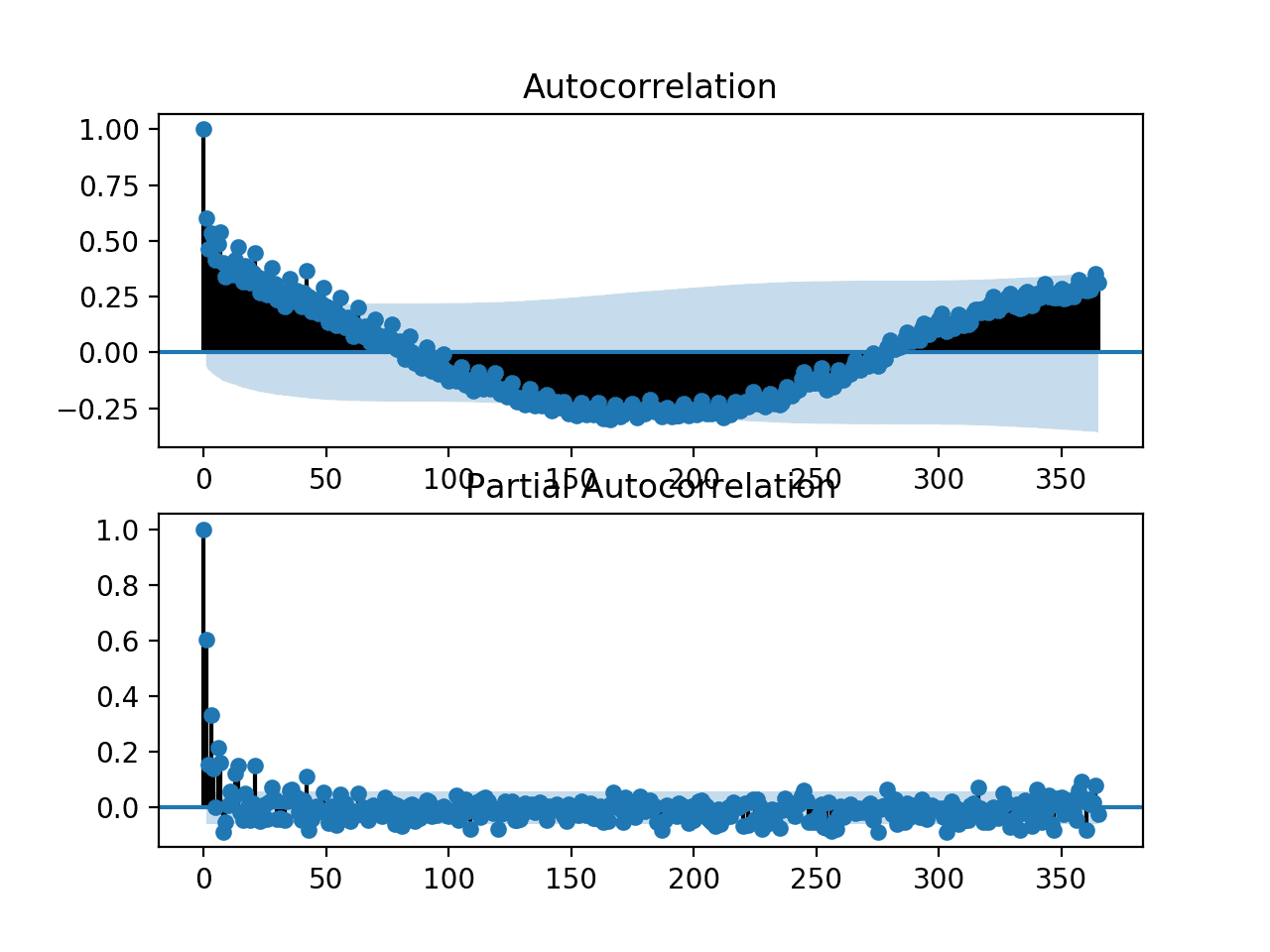
We can then create a single figure that contains both an ACF and a PACF plot. The number of lag time steps can be specified. We will fix this to be one year of daily observations, or 365 days.
1
2
3
4
5
6
7
8
9
10
11
# plots
pyplot.figure()
lags=365
# acf
axis=pyplot.subplot(2,1,1)
plot_acf(series,ax=axis,lags=lags)
# pacf
axis=pyplot.subplot(2,1,2)
plot_pacf(series,ax=axis,lags=lags)
# show plot
pyplot.show()
The complete example is listed below.
We would expect that the power consumed tomorrow and in the coming week will be dependent upon the power consumed in the prior days. As such, we would expect to see a strong autocorrelation signal in the ACF and PACF plots.
1
2
3
4
5
6
7
8
9
10
11
12
13
14
15
16
17
18
19
20
21
22
23
24
25
26
27
28
29
30
31
32
33
34
35
36
37
38
39
40
41
42
# acf and pacf plots of total power
from numpy import split
from numpy import array
from pandas import read_csv
from matplotlib import pyplot
from statsmodels.graphics.tsaplots import plot_acf
from statsmodels.graphics.tsaplots import plot_pacf
# split a univariate dataset into train/test sets
def split_dataset(data):
# split into standard weeks
train,test=data[1:-328],data[-328:-6]
# restructure into windows of weekly data
train=array(split(train,len(train)/7))
test=array(split(test,len(test)/7))
returntrain,test
# convert windows of weekly multivariate data into a series of total power
Running the example creates a single figure with both ACF and PACF plots.
The plots are very dense, and hard to read. Nevertheless, we might be able to see a familiar autoregression pattern.
We might also see some significant lag observations at one year out. Further investigation may suggest a seasonal autocorrelation component, which would not be a surprising finding.
ACF and PACF plots for the univariate series of power consumption
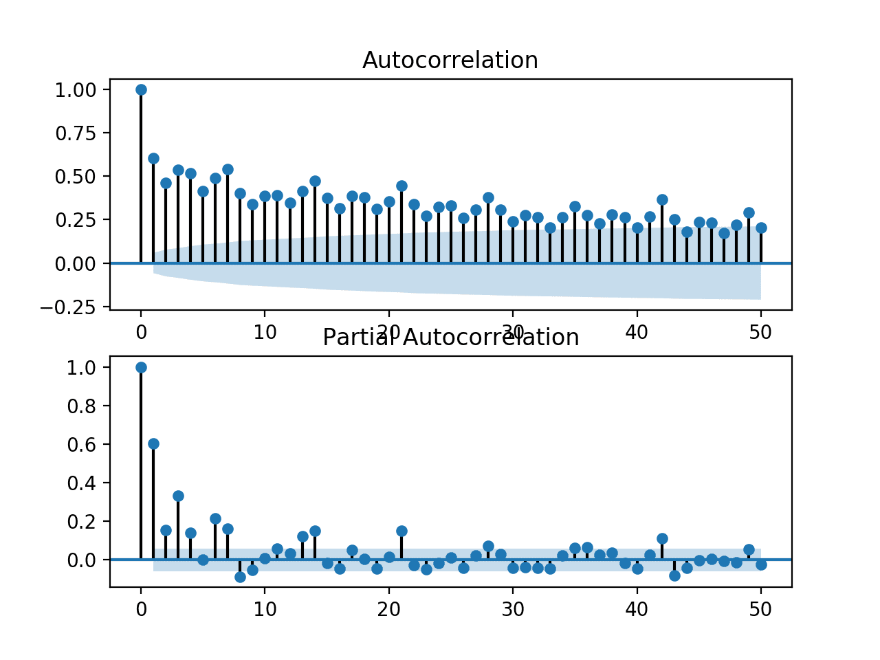
We can zoom in the plot and change the number of lag observations from 365 to 50.
1
lags=50
Re-running the code example with this change results is a zoomed-in version of the plots with much less clutter.
We can clearly see a familiar autoregression pattern across the two plots. This pattern is comprised of two elements:
ACF: A large number of significant lag observations that slowly degrade as the lag increases.
PACF: A few significant lag observations that abruptly drop as the lag increases.
The ACF plot indicates that there is a strong autocorrelation component, whereas the PACF plot indicates that this component is distinct for the first approximately seven lag observations.
This suggests that a good starting model would be an AR(7); that is an autoregression model with seven lag observations used as input.
Zoomed in ACF and PACF plots for the univariate series of power consumption
Develop an Autoregression Model
We can develop an autoregression model for univariate series of daily power consumption.
The Statsmodels library provides multiple ways of developing an AR model, such as using the AR, ARMA, ARIMA, and SARIMAX classes.
We will use the ARIMA implementation as it allows for easy expandability into differencing and moving average.
First, the history data comprised of weeks of prior observations must be converted into a univariate time series of daily power consumption. We can use the to_series() function developed in the previous section.
1
2
# convert history into a univariate series
series=to_series(history)
Next, an ARIMA model can be defined by passing arguments to the constructor of the ARIMA class.
We will specify an AR(7) model, which in ARIMA notation is ARIMA(7,0,0).
1
2
# define the model
model=ARIMA(series,order=(7,0,0))
Next, the model can be fit on the training data.
1
2
# fit the model
model_fit=model.fit()
Now that the model has been fit, we can make a prediction.
A prediction can be made by calling the predict() function and passing it either an interval of dates or indices relative to the training data. We will use indices starting with the first time step beyond the training data and extending it six more days, giving a total of a seven day forecast period beyond the training dataset.
1
2
# make forecast
yhat=model_fit.predict(len(series),len(series)+6)
We can wrap all of this up into a function below named arima_forecast() that takes the history and returns a one week forecast.
1
2
3
4
5
6
7
8
9
10
11
# arima forecast
def arima_forecast(history):
# convert history into a univariate series
series=to_series(history)
# define the model
model=ARIMA(series,order=(7,0,0))
# fit the model
model_fit=model.fit()
# make forecast
yhat=model_fit.predict(len(series),len(series)+6)
returnyhat
This function can be used directly in the test harness described previously.
The complete example is listed below.
1
2
3
4
5
6
7
8
9
10
11
12
13
14
15
16
17
18
19
20
21
22
23
24
25
26
27
28
29
30
31
32
33
34
35
36
37
38
39
40
41
42
43
44
45
46
47
48
49
50
51
52
53
54
55
56
57
58
59
60
61
62
63
64
65
66
67
68
69
70
71
72
73
74
75
76
77
78
79
80
81
82
83
84
85
86
87
88
89
90
91
92
93
94
95
96
97
98
99
# arima forecast
from math import sqrt
from numpy import split
from numpy import array
from pandas import read_csv
from sklearn.metrics import mean_squared_error
from matplotlib import pyplot
from statsmodels.tsa.arima.model import ARIMA
# split a univariate dataset into train/test sets
def split_dataset(data):
# split into standard weeks
train,test=data[1:-328],data[-328:-6]
# restructure into windows of weekly data
train=array(split(train,len(train)/7))
test=array(split(test,len(test)/7))
returntrain,test
# evaluate one or more weekly forecasts against expected values
# define the names and functions for the models we wish to evaluate
models=dict()
models['arima']=arima_forecast
# evaluate each model
days=['sun','mon','tue','wed','thr','fri','sat']
forname,func inmodels.items():
# evaluate and get scores
score,scores=evaluate_model(func,train,test)
# summarize scores
summarize_scores(name,score,scores)
# plot scores
pyplot.plot(days,scores,marker='o',label=name)
# show plot
pyplot.legend()
pyplot.show()
Running the example first prints the performance of the AR(7) model on the test dataset.
Note: Your results may vary given the stochastic nature of the algorithm or evaluation procedure, or differences in numerical precision. Consider running the example a few times and compare the average outcome.
We can see that the model achieves the overall RMSE of about 381 kilowatts.
This model has skill when compared to naive forecast models, such as a model that forecasts the week ahead using observations from the same time one year ago that achieved an overall RMSE of about 465 kilowatts.
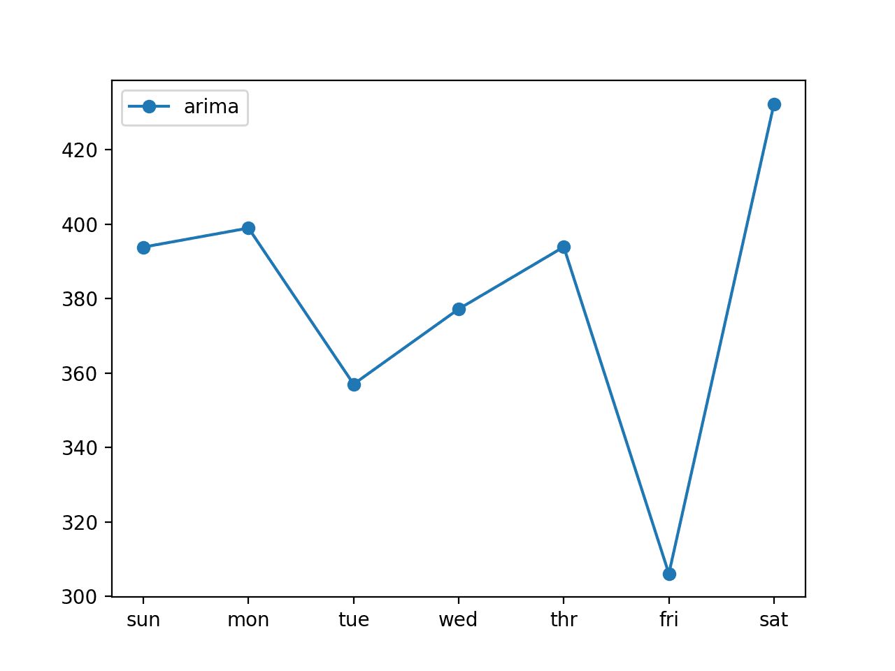
A line plot of the forecast is also created, showing the RMSE in kilowatts for each of the seven lead times of the forecast.
We can see an interesting pattern.
We might expect that earlier lead times are easier to forecast than later lead times, as the error at each successive lead time compounds.
Instead, we see that Friday (lead time +6) is the easiest to forecast and Saturday (lead time +7) is the most challenging to forecast. We can also see that the remaining lead times all have a similar error in the mid- to high-300 kilowatt range.
Line plot of ARIMA forecast error for each forecasted lead times
Extensions
This section lists some ideas for extending the tutorial that you may wish to explore.
Tune ARIMA. The parameters of the ARIMA model were not tuned. Explore or search a suite of ARIMA parameters (q, d, p) to see if performance can be further improved.
Explore Seasonal AR. Explore whether the performance of the AR model can be improved by including seasonal autoregression elements. This may require the use of a SARIMA model.
Explore Data Preparation. The model was fit on the raw data directly. Explore whether standardization or normalization or even power transforms can further improve the skill of the AR model.
If you explore any of these extensions, I’d love to know.
Further Reading
This section provides more resources on the topic if you are looking to go deeper.
the LSTM does not appear to be suitable for autoregression type problems.So this method is the best solution.But your posts have some LSTM and CNN models to solve this autoregression type problems
Hi Jason,
I am new to this data learning. I couldnt understand how you are splitting the train and test data set here
train, test = data[1:-328], data[-328:-6]
How come you took the value 328. Can you please explain me the above line of code?
The following is a recent article published Applied Energy Journal about forecasting the energy consumption of a university building based on a new hybrid neuro-fuzzy inference system boosted with a novel firefly algorithm:
The paper is entitled: A hybrid neuro-fuzzy inference system-based algorithm for time series forecasting applied to energy consumption prediction
I have reading your book on deep learning time series and it is just awesome. Everything is very well-explained.
Regarding the example above and in the book about energy consumption, I noticed that the example is for a single house. So how would you tackle the problem when you have thousands or even millions of houses?
Would it be a good idea to do a segmentation by location and get n predictions? Or it would be better to predict energy consumption of every household? (I am not sure if any ML algorithm or computer would support that large number of outcomes.)
Jason, many thanks. I checked the link provided in your reply. But I have 2 questions,
1. when you said “Develop one model for all sites” you mean generate something like this:
# Series for each household (for example for 1000 houses).
# h1 -> 1,2,3,…,n_step
# h2 -> 1,2,3,…,n_step
# h1000 -> 1,2,3,…,n_step
#create dataset
for each serie_house:
data_set = to_supervised(serie_house) #function implemented in your book
big_data_set = concatenate(big_data_set,data_set) # for rows
so big_data_set has all the supervised datasets for all houses. If that is correct, would it be a good idea to shuffle big_data_set?
2. When you say ” Develop one model per group of sites.” You meant something like this:
group 1: Low income household
group 2: high income household
Then, to model this case, should we apply the same loop as in 1?
Many thanks again and my apologies for the long message. 🙂
Hello Jason, why did you use only a univariate time series for the training of the model?
The other variable of the submetering, and the reactive power, are not important for your time series forecasting?
How to check whether our prediction is correct or not and if correct, then how much correct can we plot actual consumption and our prediction in on graph to check?


Great article. Wonder how this compares with time series forecasting with Prophet?
Thank you
Thanks.
Perhaps develop a comparison?
Great read, thanks for this.
You’re welcome.
Great work, your truly gave this forecasting an insightful overview. Thanks
Thanks Alex.
the LSTM does not appear to be suitable for autoregression type problems.So this method is the best solution.But your posts have some LSTM and CNN models to solve this autoregression type problems
Somtimes a hybrid model can perform very well.
model = ARIMA(series, order=(7,0,0))
the“7” maens lag?I have test 8 and some day perform good score as setting 7.
The results are the same for each run,while the results of in-depth learning are different each time it runs.
Yes.
What do you mean “in depth learning”?
how to set Machine precision in ARIMA()?
I note that Machine precision is 2.220D-16 in model training,but sometimes it can not Convergence
Not sure you can, not want to. It is a limitation of the libs under statsmodels.
we evaluate model in every times,model will be fitted at same time?
In the for loop, the value of history is updated at a time.
Yes, this is called walk-forward validation.
Thanks,I fund that deep learning model is not updating in every times
What do you mean exactly?
Thank you for such useful information
I’m happy that it helped.
I only have a question, why don’t you add a graph showing comparison between the predicted values and the actual real one?
Thanks for the suggestion.
If you need help making plots of forecasts, perhaps start here:
https://machinelearningmastery.com/start-here/#timeseries
Hello, may I use and modify the code and reference this article for my science project?
Yes, sounds great.
Can we use this data set and code to predict an upcoming bill?
Perhaps try it and see?
Hi Jason,
I am new to this data learning. I couldnt understand how you are splitting the train and test data set here
train, test = data[1:-328], data[-328:-6]
How come you took the value 328. Can you please explain me the above line of code?
Yes, we are using an array slice. You can learn more about array slicing in Python here:
https://machinelearningmastery.com/index-slice-reshape-numpy-arrays-machine-learning-python/
I am getting the following error
Object of type float has no len() and array split does not result in an equal division on the line
train,test = split_dataset(dataset,values)
I’m sorry to hear that, this will help:
https://machinelearningmastery.com/faq/single-faq/why-does-the-code-in-the-tutorial-not-work-for-me
Seriously, Jason, you truly are awesome . I just realised that sometimes even reading a file is not easy. but your code works like a charm
Thanks!
The following is a recent article published Applied Energy Journal about forecasting the energy consumption of a university building based on a new hybrid neuro-fuzzy inference system boosted with a novel firefly algorithm:
The paper is entitled: A hybrid neuro-fuzzy inference system-based algorithm for time series forecasting applied to energy consumption prediction
Links to the paper:
https://www.researchgate.net/publication/340824789_A_hybrid_neuro-fuzzy_inference_system-based_algorithm_for_time_series_forecasting_applied_to_energy_consumption_prediction
https://www.sciencedirect.com/science/article/abs/pii/S030626192030489X
Thanks for sharing. Why are you sharing exactly?
Hello Jason,
I have reading your book on deep learning time series and it is just awesome. Everything is very well-explained.
Regarding the example above and in the book about energy consumption, I noticed that the example is for a single house. So how would you tackle the problem when you have thousands or even millions of houses?
Would it be a good idea to do a segmentation by location and get n predictions? Or it would be better to predict energy consumption of every household? (I am not sure if any ML algorithm or computer would support that large number of outcomes.)
Many thanks, Cristina
Thank you!
Excellent question, you can develop a model to learn from behavior across houses, this will give you ideas:
https://machinelearningmastery.com/faq/single-faq/how-to-develop-forecast-models-for-multiple-sites
Many thanks Jason! I really appreciate your answer and I will check that link out.
Jason, many thanks. I checked the link provided in your reply. But I have 2 questions,
1. when you said “Develop one model for all sites” you mean generate something like this:
# Series for each household (for example for 1000 houses).
# h1 -> 1,2,3,…,n_step
# h2 -> 1,2,3,…,n_step
# h1000 -> 1,2,3,…,n_step
#create dataset
for each serie_house:
data_set = to_supervised(serie_house) #function implemented in your book
big_data_set = concatenate(big_data_set,data_set) # for rows
so big_data_set has all the supervised datasets for all houses. If that is correct, would it be a good idea to shuffle big_data_set?
2. When you say ” Develop one model per group of sites.” You meant something like this:
group 1: Low income household
group 2: high income household
Then, to model this case, should we apply the same loop as in 1?
Many thanks again and my apologies for the long message. 🙂
Perhaps.
It is open for you to interpet for your project. Perhaps experiment with a few approaches and discover what works well/best.
I am working on energy consumption data. I you dont mind to share me
rashfat2018@gmail.com
You’re welcome.
Thank you very much dear jason ..always the best
You’re welcome.
Jason ..can use the same codes for my project.. hourly energy consumption I have weather data, 20 buildings data and energy consumption data..
Sure.
Hello Jason, why did you use only a univariate time series for the training of the model?
The other variable of the submetering, and the reactive power, are not important for your time series forecasting?
Just an example.
Here’s a different example for using all the variables:
https://machinelearningmastery.com/how-to-develop-lstm-models-for-multi-step-time-series-forecasting-of-household-power-consumption/
I think walk-forward validation cheating test data. Isn’t it?
No.
How to check whether our prediction is correct or not and if correct, then how much correct can we plot actual consumption and our prediction in on graph to check?
Hi Hitesh…The following resources may add clarity:
https://deepchecks.com/how-to-check-the-accuracy-of-your-machine-learning-model/
https://vitalflux.com/steps-for-evaluating-validating-time-series-models/
Thank you I got an Idea for a performance matrix and accuracy but I still have some questions I have posted bellow
What did we predict? Energy Consumption for one week?
can we print the actual consumption data vs predicted consumption data? in on graph
can we predict for a whole month?
can we pass a data frame instead of the array throughout the program, and can we get a date-wise prediction, and how to compare it with actual data?
Hi, why did you not do outlier handling?
Hi Zaid…It was just to keep the example concise. In general you are correct that this analysis and handling should be part of every data pipeline.
Let us know if you have any questions about how to approach this topic.